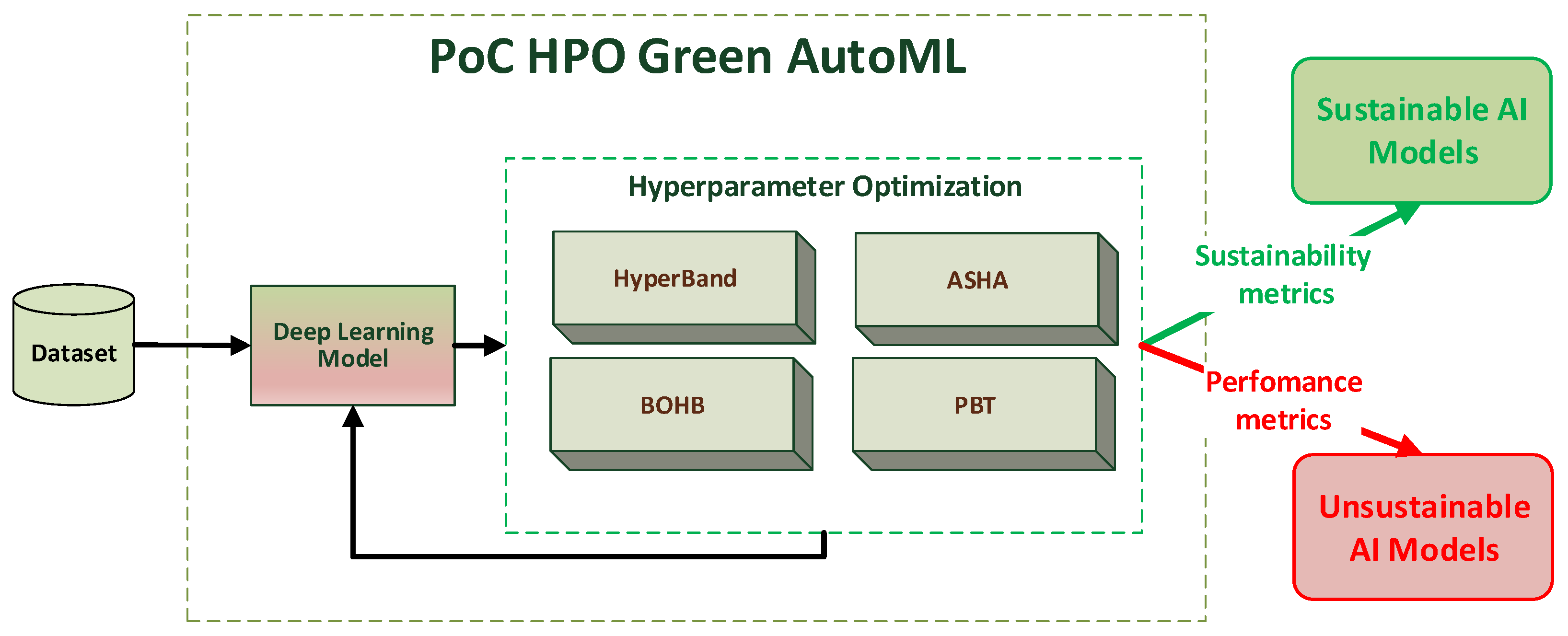
Figure 1.
The illustration depicts a workflow diagram for the proposed methodology. This workflow encompasses the input dataset and advanced algorithms for HPO, which are assessed using performance and sustainability metrics. Ultimately, high-performance artificial intelligence (AI) models are generated, or alternatively, more sustainable models are produced, facilitating the development of eco-friendly AI systems.
Figure 2.
The CO2e metric results for the 100 trials conducted by Red AI and Green AI are depicted for each algorithm. The visualization highlights the best results in terms of the CO2e metric optimization within the Green AI strategy and Red AI. The outliers represented are combinations of hyperparameters that result in solutions with high energy consumption and, consequently, with a high value of carbon dioxide equivalent. Outliers resulting from the experimentation are also presented.
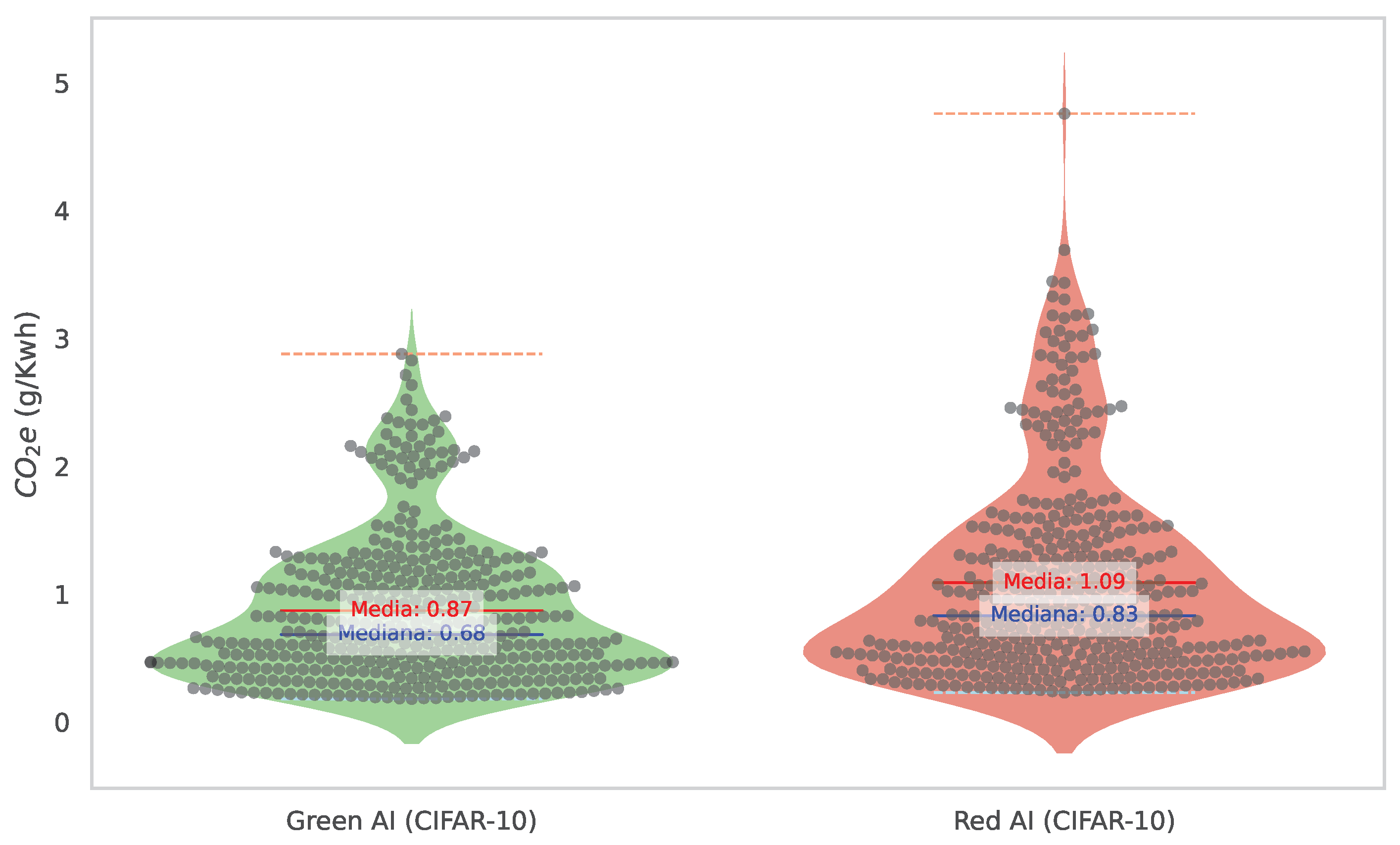
Figure 3.
The graph provides a visual representation of the distribution of the CO2e metric within the context of Green and Red artificial intelligence (AI) strategies. The results offer an in-depth view of the data density, depicted on both sides of an axis, thereby facilitating a more comprehensive understanding of the data distribution. Additionally, the figure displays the median, quartiles, and outliers of the data, offering an all-encompassing view of this metric’s distribution across both AI strategies. Outliers are combinations of hyperparameters that offer atypical solutions compared to other combinations.
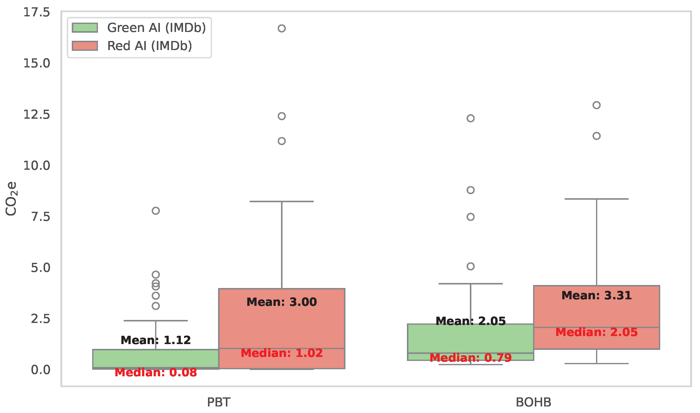
Figure 4.
The graph provides a visual representation of the distribution of the CO2e metric in the context of Green and Red artificial intelligence (AI) strategies for the IMDb dataset for the PBT and BOHB algorithms. The figure shows the median and quartiles, providing a comprehensive view of the distribution of this metric in both AI strategies. Outliers resulting from the experimentation are also presented.
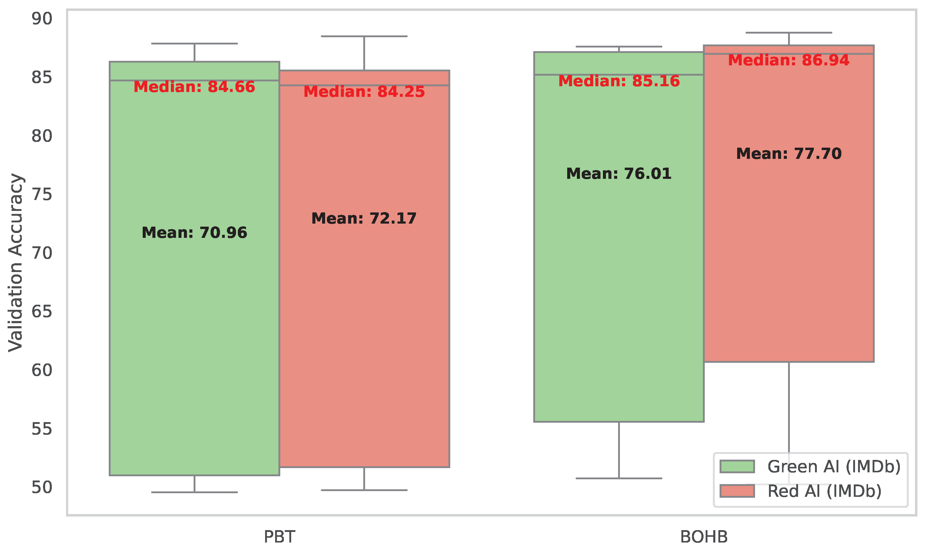
Figure 5.
The graph provides a visual representation of the distribution of the validation accuracy metric in the context of Green and Red artificial intelligence (AI) strategies for the IMDb dataset for the PBT and BOHB algorithms. The figure shows the median and quartiles, providing a comprehensive view of the distribution of this metric in both AI strategies.
Table 1.
The table elucidates the findings of the experiment conducted within the Red AI. Ten trials were executed, showing the selection of the two best and worst results, each comprising five iterations of the ASHA, BOHB, HB, and PBT algorithms, each with distinct hyperparameters. The optimized hyperparameters included learning rates (lrs) of 0.001, 0.00125, and 0.0015; epochs ranging from 5 to 20 iterations; optimizers such as Adam (AD), RMSprop (Rprop), and SGD; and batch sizes of 16, 32, and 64.
| Algorithm | Validation | (w) | Time (s) | lr | Epoch | Optimizer | Bach | CO2e |
|---|
| | Accuracy
| | | | | | |
(g/kWh)
|
|---|
| ASHA | 47.2 | 3065.44 | 506.02 | 0.0015 | 5 | AD | 16 | 0.582 |
| ASHA | 68.68 | 3300.40 | 501.50 | 0.00125 | 5 | Rprop | 16 | 0.627 |
| ASHA | 78.91 | 8729.97 | 1188.48 | 0.0015 | 20 | AD | 32 | 1.659 |
| ASHA | 80.11 | 1433.52 | 206.57 | 0.001 | 5 | Rprop | 64 | 0.272 |
| BOHB | 67.14 | 2088.49 | 299.37 | 0.001 | 5 | SGD | 32 | 0.397 |
| BOHB | 68.78 | 6096.27 | 787.88 | 0.00125 | 20 | SGD | 64 | 1.158 |
| BOHB | 79.15 | 8215.46 | 1154.96 | 0.001 | 20 | Rprop | 32 | 1.561 |
| BOHB | 81.63 | 6211.69 | 795.02 | 0.00125 | 20 | Rprop | 64 | 1.180 |
| HB | 45.45 | 4412.82 | 504.52 | 0.0015 | 5 | AD | 16 | 0.838 |
| HB | 67.02 | 18,285.95 | 1967.38 | 0.00125 | 20 | AD | 16 | 3.474 |
| HB | 79.61 | 3414.21 | 376.82 | 0.001 | 10 | Rprop | 64 | 0.649 |
| HB | 80.06 | 882.07 | 231.42 | 0.001 | 10 | Rprop | 64 | 0.168 |
| PBT | 51.63 | 3734.77 | 505.15 | 0.0015 | 5 | AD | 16 | 0.710 |
| PBT | 63.92 | 3206.16 | 474.56 | 0.00125 | 5 | SGD | 16 | 0.609 |
| PBT | 78.84 | 2020.27 | 261.97 | 0.001 | 5 | Rprop | 64 | 0.384 |
| PBT | 80.32 | 6119.05 | 782.53 | 0.001 | 20 | AD | 64 | 1.163 |
Table 2.
Comparative performance of algorithms in Red AI with 10 trials.
Table 2.
Comparative performance of algorithms in Red AI with 10 trials.
| Algorithms | CO2e (g/kWh) | Val Accuracy |
|---|
|
Std
|
Var
|
Avg
|
Median
|
Std
|
Var
|
Avg
|
Median
|
|---|
| ASHA | 0.539 | 0.290 | 0.926 | 0.868 | 9.486 | 80.984 | 72.036 | 73.915 |
| BOHB | 0.578 | 0.334 | 1.218 | 1.169 | 4.701 | 19.886 | 75.851 | 77.420 |
| HB | 1.132 | 1.281 | 1.563 | 0.738 | 10.238 | 94.326 | 70.956 | 70.280 |
| PBT | 0.447 | 0.200 | 0.854 | 1.222 | 9.078 | 74.169 | 70.502 | 71.970 |
Table 3.
Comparative performance of algorithms in Red AI with 100 trials.
Table 3.
Comparative performance of algorithms in Red AI with 100 trials.
| Algorithms | CO2e (g/kWh) | Val Accuracy |
|---|
|
Std
|
Var
|
Avg
|
Median
|
Std
|
Var
|
Avg
|
Median
|
|---|
| ASHA | 0.770 | 0.592 | 1.035 | 0.819 | 7.806 | 60.930 | 72.614 | 74.585 |
| BOHB | 0.703 | 0.494 | 0.969 | 0.763 | 8.454 | 71.477 | 72.687 | 75.850 |
| HB | 0.864 | 0.746 | 1.202 | 0.993 | 5.392 | 29.072 | 74.555 | 76.045 |
| PBT | 0.795 | 0.633 | 1.156 | 0.958 | 8.179 | 66.888 | 72.255 | 74.395 |
Table 4.
The table elucidates the findings of the experiment conducted within the Green AI. A total of ten trials were executed, showing the selection of the two best and worst results, each comprising five iterations of the ASHA, BOHB, HB, and PBT algorithms, each with distinct hyperparameters. The optimized hyperparameters included learning rates (lrs) of 0.001, 0.00125, and 0.0015; epochs ranging from 5 to 20 iterations; optimizers such as Adam (AD), RMSprop (Rprop), and SGD; and batch sizes of 16, 32, and 64.
| Algorithm | Validation | (w) | Time (s) | lr | Epoch | Optimizer | Bach | CO2e |
|---|
| |
Accuracy
| | | | | | |
(g/kWh)
|
|---|
| ASHA | 57.11 | 5419.03 | 1462.94 | 0.0015 | 20 | SGD | 16 | 1.030 |
| ASHA | 65.64 | 4169.07 | 515.17 | 0.00125 | 5 | AD | 16 | 0.792 |
| ASHA | 79.44 | 5694.30 | 732.91 | 0.001 | 20 | Rprop | 64 | 1.082 |
| ASHA | 80.08 | 5700.88 | 739.54 | 0.0015 | 20 | AD | 64 | 1.083 |
| BOHB | 64.27 | 2360.44 | 446.59 | 0.0015 | 5 | SGD | 16 | 0.448 |
| BOHB | 68.81 | 1112.85 | 182.34 | 0.001 | 5 | SGD | 64 | 0.211 |
| BOHB | 80.34 | 2646.50 | 372.06 | 0.00125 | 10 | AD | 64 | 0.503 |
| BOHB | 81.11 | 4827.45 | 720.88 | 0.001 | 20 | Rprop | 64 | 0.917 |
| HB | 39.53 | 13,085.63 | 1965.14 | 0.0015 | 20 | AD | 16 | 2.486 |
| HB | 65.31 | 851.26 | 147.24 | 0.0015 | 5 | SGD | 64 | 0.162 |
| HB | 78.82 | 7143.64 | 1077.33 | 0.00125 | 20 | AD | 32 | 1.357 |
| HB | 80.23 | 1254.59 | 325.38 | 0.0015 | 10 | Rprop | 64 | 0.238 |
| PBT | 69.01 | 1274.76 | 180.78 | 0.001 | 5 | SGD | 64 | 0.242 |
| PBT | 72.35 | 3199.51 | 480.07 | 0.001 | 5 | Rprop | 16 | 0.608 |
| PBT | 79.58 | 1390.35 | 279.76 | 0.0015 | 10 | AD | 64 | 0.264 |
| PBT | 80.22 | 2295.46 | 358.83 | 0.0015 | 10 | Rprop | 64 | 0.436 |
Table 5.
Comparative performance of algorithms in Green AI with 10 trials.
Table 5.
Comparative performance of algorithms in Green AI with 10 trials.
| Algorithms | CO2e (g/kWh) | Val Accuracy |
|---|
|
Std
|
Var
|
Avg
|
Median
|
Std
|
Var
|
Avg
|
Median
|
|---|
| ASHA | 0.565 | 0.287 | 1.059 | 0.932 | 7.538 | 51.133 | 72.750 | 74.170 |
| BOHB | 0.584 | 0.307 | 0.794 | 0.710 | 5.717 | 29.415 | 74.644 | 75.930 |
| HB | 0.723 | 0.470 | 0.811 | 0.549 | 12.357 | 137.427 | 72.323 | 78.210 |
| PBT | 0.830 | 0.621 | 0.827 | 0.522 | 3.536 | 11.251 | 76.788 | 77.630 |
Table 6.
Comparative performance of algorithms in Green AI with 100 trials.
Table 6.
Comparative performance of algorithms in Green AI with 100 trials.
| Algorithms | CO2e (g/kWh) | Val Accuracy |
|---|
|
Std
|
Var
|
Avg
|
Median
|
Std
|
Var
|
Avg
|
Median
|
|---|
| ASHA | 0.657 | 0.432 | 0.959 | 0.723 | 9.818 | 96.391 | 71.746 | 75.825 |
| BOHB | 0.512 | 0.263 | 0.809 | 0.753 | 8.457 | 71.528 | 72.924 | 75.915 |
| HB | 0.578 | 0.334 | 0.870 | 0.748 | 9.258 | 85.718 | 71.799 | 74.350 |
| PBT | 0.569 | 0.323 | 0.846 | 0.644 | 6.368 | 40.553 | 73.918 | 75.905 |
Table 7.
The table elucidates the findings of the experiment conducted within the Red AI. A total of thirty trials were executed, each comprising three iterations of the PBT algorithms, each with distinct hyperparameters. The optimized hyperparameters included maximum features ranging from 10,000 to 30,000; epochs ranging from 2 to 10 iterations; optimizers such as Adam (AD), RMSprop (Rprop), and SGD; and batch sizes of 32, 64, and 128.
| Validation | (w) | Time (s) | Max | Max | Epoch | Optimizer | Bach | CO2e |
|---|
|
Accuracy
| | |
Features
|
Len
| | | |
(g/kWh)
|
|---|
| 49.71 | 37,433.92 | 1104.51 | 30,000 | 200 | 5 | SGD | 128 | 7.112 |
| 50.14 | 11,500.53 | 308.01 | 20,000 | 300 | 2 | SGD | 64 | 2.185 |
| 50.37 | 784.58 | 1190.19 | 30,000 | 200 | 5 | SGD | 128 | 0.149 |
| 50.44 | 1465.32 | 876.20 | 10,000 | 300 | 2 | SGD | 128 | 0.278 |
| 50.60 | 12,907.44 | 362.60 | 10,000 | 300 | 2 | SGD | 32 | 2.452 |
| 50.71 | 177.67 | 331.36 | 30,000 | 300 | 2 | SGD | 64 | 0.034 |
| 51.14 | 43,252.82 | 1531.88 | 10,000 | 200 | 5 | SGD | 128 | 8.218 |
| 51.59 | 78.84 | 108.74 | 20,000 | 100 | 2 | SGD | 64 | 0.015 |
| 51.89 | 526.51 | 529.39 | 30,000 | 200 | 5 | SGD | 64 | 0.100 |
| 53.49 | 36,301.74 | 1290.10 | 10,000 | 200 | 10 | SGD | 64 | 6.897 |
| 54.80 | 20,993.73 | 692.94 | 10,000 | 100 | 10 | SGD | 32 | 3.989 |
| 54.90 | 1447.49 | 634.36 | 30,000 | 100 | 10 | SGD | 32 | 0.275 |
| 82.78 | 69.70 | 160.30 | 30,000 | 100 | 2 | Rprop | 32 | 0.013 |
| 83.39 | 36.56 | 120.64 | 30,000 | 100 | 2 | Rprop | 64 | 0.007 |
| 83.98 | 59.84 | 223.55 | 20,000 | 200 | 2 | AD | 64 | 0.011 |
| 84.53 | 3622.88 | 122.31 | 30,000 | 100 | 2 | Rprop | 128 | 0.688 |
| 84.98 | 168.72 | 221.93 | 30,000 | 100 | 5 | AD | 64 | 0.032 |
| 85.27 | 58.44 | 118.89 | 20,000 | 100 | 2 | AD | 64 | 0.011 |
| 85.28 | 244.22 | 458.85 | 20,000 | 100 | 5 | Rprop | 128 | 0.046 |
| 85.29 | 12,772.85 | 446.51 | 10,000 | 100 | 5 | Rprop | 128 | 2.427 |
| 85.32 | 203.98 | 575.88 | 10,000 | 100 | 10 | AD | 32 | 0.039 |
| 85.51 | 20,094.64 | 739.76 | 20,000 | 100 | 10 | Rprop | 64 | 3.818 |
| 85.53 | 17,832.91 | 617.82 | 30,000 | 200 | 2 | Rprop | 128 | 3.388 |
| 86.46 | 58,798.03 | 1791.48 | 10,000 | 300 | 5 | AD | 128 | 11.172 |
| 86.95 | 9827.10 | 3291.42 | 20,000 | 200 | 10 | AD | 128 | 1.867 |
| 87.46 | 709.49 | 804.46 | 30,000 | 200 | 5 | Rprop | 64 | 0.135 |
| 87.80 | 87,803.41 | 3275.55 | 30,000 | 200 | 10 | Rprop | 128 | 16.683 |
| 88.12 | 21,998.02 | 603.18 | 10,000 | 200 | 5 | Rprop | 32 | 4.180 |
| 88.36 | 7146.22 | 1923.02 | 10,000 | 300 | 10 | Rprop | 64 | 1.358 |
| 88.44 | 65,218.35 | 1934.61 | 10,000 | 300 | 10 | AD | 32 | 12.391 |
Table 8.
The table elucidates the findings of the experiment conducted within the Green AI. A total of thirty trials were executed, each comprising three iterations of the PBT algorithms, each with distinct hyperparameters. The optimized hyperparameters included maximum features ranging from 10,000 to 30,000; epochs ranging from 2 to 10 iterations; optimizers such as Adam (AD), RMSprop (Rprop), and SGD; and batch sizes of 32, 64, and 128.
| Validation | (w) | Time (s) | Max | Max | Epoch | Optimizer | Bach | CO2e |
|---|
|
Accuracy
| | |
Features
|
Len
| | | |
(g/kWh)
|
|---|
| 49.52 | 33.13 | 181.02 | 30,000 | 200 | 2 | SGD | 64 | 0.006 |
| 49.92 | 2228.96 | 209.74 | 30,000 | 200 | 2 | SGD | 32 | 0.424 |
| 49.95 | 5542.27 | 515.52 | 30,000 | 200 | 2 | SGD | 128 | 1.053 |
| 50.52 | 764.49 | 73.74 | 30,000 | 100 | 2 | SGD | 64 | 0.145 |
| 50.65 | 208.67 | 325.90 | 30,000 | 300 | 2 | SGD | 64 | 0.040 |
| 50.65 | 28.73 | 316.55 | 30,000 | 300 | 2 | SGD | 64 | 0.005 |
| 50.66 | 48.50 | 177.30 | 10,000 | 200 | 2 | SGD | 64 | 0.009 |
| 50.82 | 1911.84 | 178.27 | 20,000 | 200 | 2 | SGD | 64 | 0.363 |
| 51.36 | 26.67 | 205.24 | 20,000 | 200 | 2 | SGD | 32 | 0.005 |
| 52.11 | 22,179.18 | 2030.80 | 20,000 | 200 | 10 | SGD | 128 | 4.214 |
| 52.48 | 165.03 | 977.13 | 30,000 | 200 | 10 | SGD | 64 | 0.031 |
| 52.67 | 3676.45 | 334.12 | 10,000 | 100 | 5 | SGD | 128 | 0.699 |
| 54.17 | 18,966.34 | 1726.26 | 30,000 | 300 | 10 | SGD | 32 | 3.604 |
| 83.39 | 999.66 | 94.38 | 10,000 | 100 | 2 | Rprop | 32 | 0.190 |
| 84.64 | 125.26 | 341.75 | 30,000 | 100 | 5 | ad | 128 | 0.024 |
| 84.69 | 2871.99 | 272.41 | 10,000 | 100 | 5 | AD | 32 | 0.546 |
| 84.9 | 345.59 | 968.24 | 30,000 | 300 | 2 | Rprop | 128 | 0.066 |
| 85.22 | 66.89 | 619.44 | 30,000 | 100 | 10 | AD | 32 | 0.013 |
| 85.32 | 118.55 | 343.55 | 20,000 | 100 | 5 | AD | 128 | 0.023 |
| 85.58 | 14.89 | 99.98 | 30,000 | 100 | 2 | Rprop | 32 | 0.003 |
| 85.66 | 33.33 | 277.84 | 10,000 | 100 | 5 | Rprop | 32 | 0.006 |
| 86.16 | 24,388.97 | 2251.25 | 20,000 | 300 | 5 | AD | 128 | 4.634 |
| 86.29 | 12,543.62 | 1123.19 | 30,000 | 200 | 10 | AD | 32 | 2.383 |
| 86.38 | 330.43 | 556.33 | 20,000 | 200 | 5 | AD | 32 | 0.063 |
| 87.15 | 485.82 | 1190.38 | 10,000 | 200 | 5 | AD | 128 | 0.092 |
| 87.31 | 21,353.57 | 1926.95 | 30,000 | 300 | 5 | AD | 128 | 4.057 |
| 87.44 | 48.23 | 498.27 | 30,000 | 200 | 5 | Rprop | 64 | 0.009 |
| 87.7 | 40,846.20 | 3690.75 | 30,000 | 300 | 10 | AD | 128 | 7.761 |
| 87.77 | 16,337.37 | 1492.16 | 30,000 | 300 | 10 | Rprop | 64 | 3.104 |
| 87.81 | 122.23 | 490.41 | 10,000 | 200 | 5 | Rprop | 64 | 0.023 |
Table 9.
The table elucidates the findings of the experiment conducted within the Red AI. A total of thirty trials were executed, each comprising three iterations of the BOHB algorithms, each with distinct hyperparameters. The optimized hyperparameters included maximum features ranging from 10,000 to 30,000; epochs ranging from 2 to 10 iterations; optimizers such as Adam (AD), RMSprop (Rprop), and SGD; and batch sizes of 32, 64, and 128.
| Validation | (w) | Time (s) | Max | Max | Epoch | Optimizer | Bach | CO2e |
|---|
|
Accuracy
| | |
Features
|
Len
| | | |
(g/kWh)
|
|---|
| 50.20 | 30,212.11 | 1369.62 | 10,000 | 2000 | SGD | 32 | 5 | 5.74 |
| 50.98 | 4956.48 | 156.27 | 30,000 | 300 | SGD | 64 | 5 | 0.942 |
| 51.38 | 1507.00 | 47.21 | 10,000 | 100 | SGD | 64 | 2 | 0.286 |
| 51.80 | 20,541.84 | 713.15 | 30,000 | 2000 | SGD | 64 | 5 | 3.903 |
| 51.84 | 1859.32 | 56.88 | 20,000 | 100 | SGD | 128 | 5 | 0.353 |
| 52.30 | 4861.84 | 122.80 | 20,000 | 300 | SGD | 128 | 5 | 0.924 |
| 52.36 | 32,433.27 | 1471.54 | 10,000 | 2000 | SGD | 32 | 5 | 6.162 |
| 52.58 | 43,899.18 | 1333.07 | 20,000 | 2000 | SGD | 64 | 10 | 8.341 |
| 84.82 | 4379.05 | 117.07 | 30,000 | 100 | AD | 128 | 10 | 0.832 |
| 85.28 | 4886.98 | 143.89 | 20,000 | 100 | Rprop | 64 | 10 | 0.929 |
| 85.39 | 2465.77 | 95.36 | 10,000 | 100 | Rprop | 64 | 5 | 0.468 |
| 86.17 | 10,544.97 | 337.84 | 20,000 | 300 | AD | 64 | 10 | 2.004 |
| 86.28 | 9402.99 | 343.67 | 20,000 | 2000 | AD | 64 | 2 | 1.787 |
| 86.84 | 9573.21 | 308.11 | 20,000 | 300 | AD | 32 | 5 | 1.819 |
| 86.92 | 6268.75 | 207.86 | 10,000 | 300 | AD | 64 | 5 | 1.191 |
| 86.95 | 16,685.24 | 616.88 | 20,000 | 300 | AD | 32 | 10 | 3.17 |
| 86.97 | 14,972.11 | 661.55 | 20,000 | 2000 | AD | 32 | 2 | 2.845 |
| 87.39 | 21,227.97 | 981.87 | 30,000 | 2000 | AD | 128 | 10 | 4.033 |
| 87.44 | 32,236.47 | 971.46 | 20,000 | 2000 | AD | 128 | 10 | 6.125 |
| 87.48 | 11,062.88 | 330.84 | 20,000 | 2000 | AD | 64 | 2 | 2.102 |
| 87.50 | 14,197.34 | 492.86 | 10,000 | 2000 | AD | 128 | 5 | 2.697 |
| 87.55 | 13,350.97 | 509.96 | 30,000 | 2000 | AD | 128 | 5 | 2.537 |
| 87.68 | 5943.76 | 180.63 | 30,000 | 300 | Rprop | 64 | 5 | 1.129 |
| 87.80 | 6808.25 | 213.08 | 10,000 | 2000 | AD | 128 | 2 | 1.294 |
| 87.95 | 2323.36 | 74.71 | 30,000 | 300 | AD | 128 | 2 | 0.441 |
| 87.96 | 37,971.15 | 1356.75 | 10,000 | 2000 | AD | 32 | 5 | 7.215 |
| 88.08 | 60,120.23 | 2608.80 | 10,000 | 2000 | AD | 32 | 10 | 11.423 |
| 88.14 | 21,655.02 | 715.80 | 10,000 | 2000 | Rprop | 64 | 5 | 4.114 |
| 88.15 | 8141.40 | 268.05 | 10,000 | 300 | Rprop | 32 | 5 | 1.547 |
| 88.74 | 68,038.37 | 2610.30 | 30,000 | 2000 | Rprop | 32 | 10 | 12.927 |
Table 10.
The table elucidates the findings of the experiment conducted within the Green AI. A total of thirty trials were executed, each comprising three iterations of the BOHB algorithms, each with distinct hyperparameters. The optimized hyperparameters included maximum features ranging from 10,000 to 30,000; epochs ranging from 2 to 10 iterations; optimizers such as Adam (AD), RMSprop (Rprop), and SGD; and batch sizes of 32, 64, and 128.
| Validation | (w) | Time (s) | Max | Max | Epoch | Optimizer | Bach | CO2e |
|---|
|
Accuracy
| | |
Features
|
Len
| | | |
(g/kWh)
|
|---|
| 50.71 | 1239.15 | 47.43 | 10,000 | 100 | 2 | SGD | 64 | 0.235 |
| 51.06 | 6568.25 | 269.55 | 20,000 | 300 | 5 | SGD | 32 | 1.248 |
| 52.02 | 16,534.06 | 494.55 | 10,000 | 300 | 10 | SGD | 32 | 3.141 |
| 52.32 | 7881.13 | 280.74 | 10,000 | 300 | 5 | SGD | 32 | 1.497 |
| 52.33 | 4198.72 | 104.58 | 10,000 | 300 | 5 | SGD | 128 | 0.798 |
| 52.54 | 39,271.67 | 1264.49 | 30,000 | 2000 | 5 | SGD | 32 | 7.462 |
| 53.27 | 4319.18 | 132.45 | 20,000 | 100 | 10 | SGD | 64 | 0.821 |
| 55.32 | 3281.47 | 139.56 | 10,000 | 100 | 10 | SGD | 64 | 0.623 |
| 56.2 | 64,652.37 | 2390.88 | 10,000 | 2000 | 10 | SGD | 32 | 12.284 |
| 80.45 | 1277.27 | 43.1 | 20,000 | 100 | 2 | Rprop | 128 | 0.243 |
| 84.25 | 2651.41 | 141.34 | 30,000 | 100 | 5 | Rprop | 32 | 0.504 |
| 84.38 | 2081.01 | 59.62 | 10,000 | 100 | 5 | Rprop | 128 | 0.395 |
| 84.49 | 1890.48 | 76.92 | 10,000 | 100 | 2 | AD | 32 | 0.359 |
| 84.63 | 4143.16 | 154.09 | 20,000 | 100 | 10 | AD | 64 | 0.787 |
| 85.12 | 2231.29 | 70.12 | 10,000 | 100 | 5 | AD | 128 | 0.424 |
| 85.19 | 3435.22 | 98.1 | 30,000 | 100 | 10 | Rprop | 128 | 0.653 |
| 85.28 | 1846.09 | 60.68 | 30,000 | 300 | 2 | Rprop | 128 | 0.351 |
| 85.38 | 3129.63 | 144.08 | 20,000 | 100 | 5 | Rprop | 32 | 0.595 |
| 86.23 | 2160.13 | 73.28 | 30,000 | 300 | 2 | AD | 128 | 0.41 |
| 86.78 | 5235.87 | 133.2 | 30,000 | 300 | 5 | AD | 128 | 0.995 |
| 86.82 | 3632.52 | 129.11 | 10,000 | 300 | 2 | Rprop | 32 | 0.69 |
| 86.94 | 2044.75 | 57.46 | 10,000 | 300 | 2 | Rprop | 128 | 0.389 |
| 87.15 | 22,058.11 | 918.94 | 30,000 | 2000 | 10 | Rprop | 128 | 4.191 |
| 87.18 | 11,013 | 316 | 30,000 | 2000 | 2 | AD | 64 | 2.092 |
| 87.22 | 11,889.38 | 303.38 | 10,000 | 300 | 10 | AD | 64 | 2.259 |
| 87.28 | 4541.17 | 165.07 | 30,000 | 300 | 5 | Rprop | 64 | 0.863 |
| 87.32 | 26,534.06 | 936.43 | 10,000 | 2000 | 10 | AD | 128 | 5.041 |
| 87.44 | 15,022.42 | 464.5 | 30,000 | 2000 | 5 | Rprop | 128 | 2.854 |
| 87.45 | 3314.13 | 105.16 | 30,000 | 300 | 2 | AD | 64 | 0.63 |
| 87.55 | 46,168.17 | 1370.24 | 30,000 | 2000 | 10 | Rprop | 64 | 8.772 |


