A Galerkin Finite Element Method for the Reconstruction of a Time-Dependent Convection Coefficient and Source in a 1D Model of Magnetohydrodynamics

Abstract

The mathematical analysis of viscous magnetohydrodynamics (MHD) models is of great interest in recent years. In this paper, a finite element Galerkin method is employed for the estimation of an unknown time-dependent convection coefficient and source in a 1D magnetohydrodynamics flow system. In this inverse problem, two integral observations are posed and used to transform the inverse problem to a non-classical direct problem with a non-local parabolic operator. Then, the non-classical strongly coupled parabolic system is studied in various settings. The equivalence of the inverse problem (IP) and the direct one are proven. The Galerkin procedure is analyzed to proove the existence and uniqueness of the solution. The finite element method (FEM) has been developed for the solution of the variational problem. Test examples are discussed.

1. Introduction

Viscous MHD duct flows present significant challenges and are of great interest in both physics and engineering due to their substantial theoretical and practical importance. They have widespread applications in various fields such as astrophysics, geology, biology, in the design of cooling systems using liquid metals for nuclear fission or fusion reactors, power generation, MHD generators, and electromagnetic pumps. Therefore, it is not surprising that numerous theoretical and experimental studies have been conducted on these issues over the past decades.

Solving the equations governing MHD flows is quite challenging due to the coupling between fluid mechanics and electrodynamics equations. Consequently, analytical solutions are only available for specific cases. Therefore, in general, MHD flow problems must be solved numerically using various numerical techniques [1,2,3,4,5].

Biological effect of magnetic field is discovered during the last decades [6]. From a physical point of view, one evident phenomenon is the magnetic alignment observed in biological systems [7]. Application of MHD problems and their numerical modelling in biological systems are discussed in [8,9].

Hydrodynamic model simulations are very important in forecasting the environmental fate and potential environmental consequences of chemical contaminants, see e.g., [10]. The authors created a hydrodynamic model to predict and assess the risk of chemical contaminants in Xiamen Bay. The book by [11] is devoted to the mathematical theory of climate and atmospheric pollution and application. In particular, ref. [12] numerically studied a general hydrodynamical model of air circulation, including magnetic fields.

The laser-induced wave propagation and reflection phenomenon in a functionally graded porous medium subjected to an electro-magnetic field was investigated in [13], utilizying FEM. In [14] the authors used FEM to develope and numericaly solve new nonlinear coupled finite-strain electro-magneto-thermo-hyperelasticity molels. The governing equations were derived in line with a nonlinear version of the Helmholtz free energy.

While steady MHD duct flows have been extensively studied, there are less papers focusing on unsteady, two-dimensional, incompressible, viscous MHD flow in channels.

Studies on time-dependent MHD flow systems, focusing on flow control and MHD stability, have addressed various issues. These control and stability problems for MHD flows are all model-based approaches, where the model parameters or initial conditions are assumed to be well-defined. However, when these model parameters (i.e., empirical parameters and initial conditions) are not precisely known or are uncertain, it typically leads to biased simulation results and inconsistencies between the output of the established control system and the actual physical system.

Therefore, it is crucial to identify these unknown or uncertain parameters in the direct system model to ensure that the mathematical model accurately represents the real physical system under consideration. These challenges are commonly known as parameter estimation problems or inverse problems in the field of data assimilation.

In this paper, we address a reconstruction problem for a simplified MHD Hartmann flow characterized by incompressible and Newtonian (constant viscosity) properties in a 1D space. The mathematical model for the 1D MHD Hartmann flow can be effectively constructed under certain suitable assumptions, tightly coupling the flow velocity and electromagnetic fields [2,3,4,5].

Control and stability issues for MHD flows have been investigated over the past few decades, see, e.g., [1,2,3,4,5]. Identifying various unknown or uncertain parameters in the differential problem is crucial for ensuring that the mathematical model accurately represents the physical phenomena under study. This lack of information must be addressed by solving inverse problems.

In the paper by [3], an adjoint-based optimization method is used to estimate the unknown coefficients and states in a one-dimensional magnetohydrodynamics flow. This approach involves gradient-like search methods, which are time-consuming. In the article by [15], the coefficient and source inverse problem is transformed into a non-classical forward problem. The loaded equation method was utilized in [16], and the finite difference solution of the transformed problem was implemented.

In the present work, we consider the estimation of the convection coefficient and source in 1D MHD flow system upon two space integral observations. The problem of finding time right-hand sides and time-dependent coefficients for parabolic and hyperbolic equations are widely studied; see, e.g., [17,18,19,20,21,22,23,24,25,26,27,28]. We also work in the same way as the authors of [15] with the transformed non-classical forward problems. We define a variational formulation for these problems; then, the continuous and discrete Galerkin procedures are studied. Numerical test examples are performed to clarify the theoretical results.

The rest of the paper is organized as follows. In the next section, the forward (direct) and inverse problems are described. In Section 3, we construct the equivalents to the inverse problems for non-classical forward ones and their variational forms. The continuous Galerkin approximations for the non-classical problems are studied in Section 4. A finite element realization of the Galerkin procedures is discussed in Section 5. The computational results are analyzed in Section 5.1 and then the paper is finalized by the conclusions.

2. The Direct and Inverse Problems

For the description of the dynamic model, we followed [2,3,4,5]. We considered a simplified MHD Hartman flow with incompressible and Newtonian (constant viscosity) characteristics in 1D space as well as a case in which the fluid flowed between two parallel solid plates and where the velocity was perpendicular to the magnetic vector. Moreover, the pressure in the channel was supposed to be constant and the unit vectors of velocity, the mathematical model describing this 1D MHD flow system, could be derived from the viscous incompressible MHD equations [2,3,4,5]. It reads as follows:

$$\begin{array}{ccc}& & \frac{\partial u}{\partial t}-\nu \frac{{\partial }^{2}u}{\partial x^2}=\beta \left(t\right)\frac{\partial B}{\partial x}-f\left(t\right),\hfill \end{array}$$

(1)

$$\begin{array}{ccc}& & \frac{\partial B}{\partial t}-{\nu }_m\frac{{\partial }^{2}B}{\partial x^2}=\beta \left(t\right)\frac{\partial u}{\partial x}.\hfill \end{array}$$

(2)

Here, the spatial variable x and time variable t belong to the set $(x,t)\in Q_T=\Omega \times (O,T)$, where $\Omega =(0,1)$. In this context, $u(x,t)$ denotes the flow velocity, $B(x,t)$ is the magnetic field, $f\left(t\right)$ is the pressure difference per unit length of the channel, and the function $\beta \left(t\right)$ is a given function of the induction of the extended magnetic fields, which can be considered as the control input for the MHD flow. Additionally, $\nu$ and ${\nu }_m$ are two positive kinetic viscosity coefficients.

In [3], it is assumed that the boundary conditions on the magnetic on the solid surfaces are zero velocity for the viscous fluid and zero boundary conditions for the magnetic field, corresponding to the continuity of the magnetic field strength. Thus, the boundary conditions for system (1) and (2) are given as follows:

$$\begin{array}{ccc}& & u(0,t)=u_l\left(t\right),u(1,t)=u_r\left(t\right),\hfill \end{array}$$

(3)

$$\begin{array}{ccc}& & B(0,t)=B_l\left(t\right),B(1,t)=B_r\left(t\right).\hfill \end{array}$$

(4)

Furthermore, the initial conditions for the dynamic system (1), (2) are provided by

$$u(x,0)=u_0\left(x\right),B(x,0)=B_0\left(x\right).$$

(5)

In the form (1)–(5), we pose the direct (forward) problem, in which the right-hand sides, coefficients, boundary conditions, and initial conditions are given.

Consider the inverse problem in which the coefficient $\beta \left(t\right)$ and the source $f\left(t\right)$ are unknowns, along with the over-specified total energy condition.

$${\int }_0^{1}u(x,t)dx=E\left(t\right),$$

(6)

and total magnetic energy

$${\int }_0^{1}B(x,t)dx=F\left(t\right).$$

(7)

Here, $E\left(t\right)$ and $F\left(t\right)$ are the given functions.

Least squares is often used to define the closeness (objective functional). The resulting methods are referred to as the least squares output error criteria procedures; see, e.g., [3]. Although these procedures have many advantages, they also have drawbacks. For example, they are computationally intensive because iterative procedures (such as gradient-like search) are used. In addition, each step in the iteration reduces to solving a forward problem which involves the numerical solution of partial differential equations. Thus, there is a clear need to minimize the number of steps in the iteration, as well as to reduce the range of the global search. One way this can be achieved is to obtain an independent initial estimate of the structure of the control parameters. In the present work, our goal is to construct an efficient numerical procedure. We transform the identification problem for recovering time-dependent functions $\beta \left(t\right),f\left(t\right)$ into a non-classical forward problem.

3. Reduction of the Inverse Problem to a Non-Classical Forward Problem

The following requirements for the input data of the problem are assumed in the rest of the paper.

H1. 

Functions $E\left(t\right)$ and $F\left(t\right)$ belong to class $C^1[0,T]$;  

H2. 

The boundary conditions (3), (4) satisfy

$$u_r\left(t\right)\ne u_l\left(t\right),B_r\left(t\right)\ne B_l\left(t\right),\mathrm{for}\mathrm{each}t\in [0,T].$$

3.1. Reducing the Inverse Problem to a Direct One

If we differentiate $F\left(t\right)$ with respect to t and use the Equation (2), we obtain

$${\int }_0^1\left({\nu }_m\frac{{\partial }^{2}B}{\partial x^2}+\beta \left(t\right)\frac{\partial u}{\partial x}\right)dx=F^{\prime }\left(t\right),F^{\prime }\left(t\right)=\frac{dF}{dt}.$$

Then, taking into account the boundary conditions (4), we derive

$$\beta \left(t\right)=\frac{F^{\prime }\left(t\right)-{\nu }_m\left(B_x(1,t)-B_x(0,t)\right)}{g_u\left(t\right)},g_u\left(t\right)=u_r\left(t\right)-u_l\left(t\right).$$

(8)

where ${\displaystyle B_x=\frac{\partial B}{\partial x}}$. Next, in the same manner, differentiating $E\left(t\right)$ with respect to t and using the Equation (1) and boundary conditions (3), we find

$$f\left(t\right)=\nu \left(u_x(1,t)-u_x(0,t)\right)+\beta \left(t\right)g_B\left(t\right)-E^{\prime }\left(t\right),g_B\left(t\right)=B_r\left(t\right)-B_l\left(t\right).$$

(9)

Further, we define

$$\begin{array}{ccc}& & U(x,t)=u(x,t)-\widehat{u}\left(t\right),\widehat{u}(x,t)=(1-x)u_l\left(t\right)+x{u}_r\left(t\right),\hfill \end{array}$$

(10)

$$\begin{array}{ccc}& & b(x,t)=B(x,t)-\widehat{B}(x,t),\widehat{B}(x,t)=(1-x)B_l\left(t\right)+x{B}_r\left(t\right).\hfill \end{array}$$

(11)

Using the transformation (10), (11), the problem (1)–(5) can be written in the non-classical form

$$\begin{array}{ccc}& & \frac{\partial U}{\partial t}-\nu \frac{{\partial }^{2}U}{\partial x^2}=\beta \left(t\right)\frac{\partial b}{\partial x}-\frac{\partial \widehat{u}}{\partial t}(x,t)-\beta \left(t\right)g_B\left(t\right)-f\left(t\right),\hfill \end{array}$$

(12)

$$\begin{array}{ccc}& & \frac{\partial b}{\partial t}-{\nu }_m\frac{{\partial }^{2}b}{\partial x^2}=\beta \left(t\right)\frac{\partial U}{\partial x}-\frac{\partial \widehat{B}}{\partial t}(x,t)-\beta \left(t\right)g_u\left(t\right),\hfill \end{array}$$

(13)

$$\begin{array}{ccc}& & U(0,t)=0,U(1,t)=0,\hfill \end{array}$$

(14)

$$\begin{array}{ccc}& & b(0,t)=0,b(1,t)=0,\hfill \end{array}$$

(15)

$$\begin{array}{ccc}& & U(x,0)=u_0\left(x\right)-\widehat{u}(x,0)=U_0\left(x\right),\hfill \end{array}$$

(16)

$$\begin{array}{ccc}& & b(x,0)=B_0\left(x\right)-\widehat{B}(x,0)=b_0\left(x\right).\hfill \end{array}$$

(17)

Now, in view of (8)–(11), $\beta \left(t\right)$ and $f\left(t\right)$ are already provided by

$$\begin{array}{ccc}& & \beta \left(t\right)=\frac{F^{\prime }\left(t\right)-{\nu }_m(b_x(1,t)-b_x(0,t))}{g_u\left(t\right)},\hfill \end{array}$$

(18)

$$\begin{array}{ccc}& & f\left(t\right)=\nu \left(U_x(1,t)-U_x(0,t)\right)+\beta \left(t\right)g_B\left(t\right)-E^{\prime }\left(t\right).\hfill \end{array}$$

(19)

The following theorem is a result of the above constructions.

Theorem 1. 

Let $u_0\left(x\right),B_0\left(x\right)\in C^1(\Omega )$ and hypotheses H1 and H2 hold. Then, the IP (1)–(7) is equivalent to the forward problem (8)–(19).

Proof. 

The proof directly follows from the constructions in Section 3.1.   □

3.2. Variational Formulation

Let us introduce the functions

$$v(x,t)=\frac{\partial U}{\partial x}(x,t),w(x,t)=\frac{\partial b}{\partial x}(x,t).$$

(20)

In order to construct a weak formulation for $(v,\phi ):={\int }_0^{1}v\phi dx$, where $\phi$ is a function of $H^1(\Omega )$, we form the inner product of (12) with ${\phi }_x$ and integrate by parts with respect to x, using the boundary conditions (14). We perform the same procedure for the pair $(b,\phi )$. As a result, we obtain

$$\begin{array}{c}\hfill \begin{array}{cc}\hfill & \left(\frac{\partial v}{\partial t},\phi \right)+\nu \left(\frac{\partial v}{\partial x},{\phi }_x\right)=\beta \left(t\right)\left(w,{\phi }_x\right)+\beta \left(t\right)(\phi \left(1\right)-\phi \left(0\right))g_B\left(t\right)\hfill \\ & -f\left(t\right)(\phi \left(1\right)-\phi \left(0\right))-\left(\frac{\partial \widehat{u}}{\partial t},{\phi }_x\right),\hfill \\ & \left(\frac{\partial w}{\partial t},\phi \right)+{\nu }_m\left(\frac{\partial w}{\partial x},{\phi }_x\right)=\beta \left(t\right)\left(v,{\phi }_x\right)+\beta \left(t\right)(\phi \left(1\right)-\phi \left(0\right))g_u\left(t\right)\hfill \\ & -\left(\frac{\partial \widehat{B}}{\partial t},{\phi }_x\right),\hfill \\ & (v(x,0),\phi )=\left(\frac{d{U}_0}{dx},\phi \right),(w(x,0),\phi )=\left(\frac{d{b}_0}{dx},\phi \right).\hfill \end{array}\end{array}$$

(21)

According to (18)–(20), we obtain

$$\begin{array}{ccc}& & \beta \left(t\right)=\frac{F^{\prime }\left(t\right)-{\nu }_m(w(1,t)-w(0,t))}{g_u\left(t\right)},\hfill \end{array}$$

(22)

$$\begin{array}{ccc}& & f\left(t\right)=\nu \left(v(1,t)-v(0,t)\right)+\beta \left(t\right)g_B\left(t\right)-E^{\prime }\left(t\right).\hfill \end{array}$$

(23)

Theorem 2. 

Let the assumptions of Theorem 1 hold. Then, if $\left\{v\right(x,t),w(x,t\left)\right\}$ is a variational solution of (21)–(23), then the pair $\left\{U\right(x,t),b(x,t\left)\right\}$ is a solution to the problem (12)–(19) and vice versa.

Proof. 

From the assumptions of the theorem, it follows that $v=\frac{\partial U}{\partial x}\in H^1(\Omega )$, $w=\frac{\partial b}{\partial x}\in H^1(\Omega )$; which is the solution to the variational problem (21) and (22).

Conversely, the sufficient smoothness of the variational solution of (21) and (22) assures the solution of the forward problem (12)–(19).    □

Therefore, if one can obtain an approximate solution of the variational problem (21)–(23), one also has an approximate solution to the original problem (12)–(19). Thus, in the next section, we concentrate on the Galerkin and finite element numerical solution of the variational problem.

4. Continuous Galerkin Approximation

In this section, we use the well-known inequalities, see, e.g., [29,30]: the $\epsilon$ inequality

$$ab\le \epsilon a^2+\frac{b^2}{4\epsilon },\epsilon >0$$

and trace estimates

$$\begin{array}{ccc}& & {\psi }^2\left(0\right)\le \epsilon {∥\frac{d\psi }{dx}∥}^2+C_1{\epsilon }^{-1}{\parallel \psi \parallel }^2,0<\epsilon <{\epsilon }_0,\hfill \\ & & {\psi }^2\left(1\right)\le \epsilon {∥\frac{d\psi }{dx}∥}^2+C_2{\epsilon }^{-1}{\parallel \psi \parallel }^2,\hfill \end{array}$$

where

$$\psi =\psi \left(x\right),x\in {[0,1],\parallel \psi \parallel }^2=\underset{0}{\overset{1}{\int }}{\left|\psi \left(x\right)\right|}^{2}dx.$$

Let ${\left\{{\phi }_i\left(x\right)\right\}}_{i=1}$ be a set of linearly independent functions that are defined and continuously differentiable over $0\le x\le 1$.

Let ${\Phi }_N=\mathrm{span}\{{\phi }_1,\cdots ,{\phi }_N\}$ and

$$\begin{array}{ccc}\hfill S^N& =& C^1([0,T];{\Phi }_N)\hfill \\ & =& \{P(x,t):P(x,t)=\sum _{i=1}^N{p}_i\left(t\right){\phi }_i\left(x\right)\mathrm{with}{p}_k\left(t\right)\in C^1[0,T],k=1,\cdots ,N\}.\hfill \end{array}$$

To approximate $V(x,t)$ by functions $V(x,t)={\sum }_{i=1}^N{v}_i\left(t\right){\phi }_i\left(x\right)\in S^N$ and $W(x,t)={\sum }_{i=1}^N{w}_i\left(t\right){\phi }_i\left(x\right)\in S^N$, respectively, we formulate the continuous Galerkin approximation of the problem (21)–(23) as follows:

$$\begin{array}{ccc}\hfill \left(\frac{\partial V}{\partial t},\Phi \right)+\nu \left(\frac{\partial V}{\partial x},\frac{\partial \Phi }{\partial x}\right)& =& \tilde{\beta }\left(t\right)\left(\frac{\partial W}{\partial x},\Phi \right)+\tilde{\beta }\left(t\right)(\Phi (1,t)-\Phi (0,t))g_B\left(t\right)\hfill \end{array}$$

$$\begin{array}{ccc}& & -\tilde{f}\left(t\right)(\Phi (1,t)-\Phi (0,t))-\left(\frac{\partial \widehat{u}}{\partial t},{\Phi }_x\right),\hfill \\ \hfill \left(\frac{\partial W}{\partial t},\Phi \right)+{\nu }_m\left(\frac{\partial W}{\partial x},\frac{\partial \Phi }{\partial x}\right)& =& \tilde{\beta }\left(t\right)\left(\frac{\partial V}{\partial x},\Phi \right)+\tilde{\beta }\left(t\right)(\Phi (1,t)-\Phi (0,t))g_u\left(t\right)\hfill \end{array}$$

(24)

$$\begin{array}{ccc}& & -\left(\frac{\partial \widehat{B}}{\partial t},{\Phi }_x\right),\hfill \end{array}$$

(25)

where

$$\tilde{\beta }\left(t\right)=\frac{F^{\prime }\left(t\right)-{\nu }_m(W(1,t)-W(0,t))}{g_u\left(t\right)},\tilde{f}\left(t\right)=\nu \left(V(1,t)-V(0,t)\right)+\tilde{\beta }\left(t\right)g_B\left(t\right)-E^{\prime }\left(t\right)$$

and

$$(U,\Phi )=\left(\frac{d{U}_0}{dx},\Phi \right),(V,\Phi )=\left(\frac{d{b}_0}{dx},\Phi \right),t=0,\forall \Phi \in S^N.$$

(26)

Theorem 3. 

Under the conditions $H1$ and $H2$, the variational problem (24)–(26) has a unique solution.

Proof. 

First, we show the uniqueness.

Assume that the pairs $\left(V\right(x,t),W(x,t\left)\right)$ and $(V^{\ast }(x,t),W^{\ast }(x,t))$ are two finite element solutions of the problem (24)–(26)

Let

$$Y(x,t),=V(x,t)-V^{\ast }(x,t),Z(x,t)=W(x,t)-W^{\ast }(x,t),(x,t)\in {\overline{Q}}_T.$$

Obviously, $Y(x,t)\in S^N$, $Z(x,t)\in S^N$. Subtract the equation for $V^{\ast }(x,t)$ from the equation for $V(x,t)$ and subtract the equation for $W^{\ast }(x,t)$ from the equation for $W(x,t)$. From a direct calculation, it can be seen that

$$\begin{array}{c}\hfill \begin{array}{cc}\hfill \left(\frac{\partial Y}{\partial t},\Phi \right)+\nu \left(\frac{\partial Y}{\partial x},\frac{\partial \Phi }{\partial x}\right)=& ▵\tilde{\beta }\left(\frac{\partial W}{\partial x},\Phi \right)+{\tilde{\beta }}^{\ast }\left(t\right)\left(\frac{\partial Z}{\partial x},\Phi \right)\hfill \\ \hfill & +▵\tilde{\beta }(\Phi (1,t)-\Phi (0,t))-▵\tilde{f}(\Phi (1,t)-\Phi (0,t))\hfill \end{array}\end{array}$$

(27)

$$\begin{array}{c}\hfill \begin{array}{cc}\hfill \left(\frac{\partial Z}{\partial t},\Phi \right)+{\nu }_m\left(\frac{\partial Z}{\partial x},\frac{\partial \Phi }{\partial x}\right)=& ▵\tilde{\beta }\left(\frac{\partial W}{\partial x},\Phi \right)+{\tilde{\beta }}^{\ast }\left(t\right)\left(\frac{\partial Y}{\partial x},\Phi \right)\hfill \\ \hfill & +▵\tilde{\beta }(\Phi (1,t)-\Phi (0,t)),\hfill \end{array}\end{array}$$

(28)

where

$$\begin{array}{ccc}\hfill & & ▵\tilde{\beta }=\tilde{\beta }\left(t\right)-{\tilde{\beta }}^{\ast }\left(t\right)=\frac{-{\nu }_m}{g_u\left(t\right)}(Z(1,t)-Z(0,t)),\hfill \\ \hfill & & ▵\tilde{f}=\tilde{f}\left(t\right)-{\tilde{f}}^{\ast }\left(t\right)=\nu (Y(1,t)-Y(0,t))+{\nu }_m\frac{g_B\left(t\right)}{g_u\left(t\right)}(Z(1,t)-Z(0,t)),\hfill \end{array}$$

and

$$(Y,\Phi )=0,(Z,\Phi )=0.$$

We take $\varphi =Y$ as a test function in (27) and $\varphi =Z$ as a test function in (28). We have

$$\left(\frac{dY}{dt},Y\right)=\frac{1}{2}\frac{d}{dt}{\parallel Y\parallel }^2,\left(\frac{\partial Z}{\partial t},Z\right)=\frac{1}{2}\frac{d}{dt}{\parallel Z\parallel }^2.$$

In view of the trace inequalities, we find:

$$\parallel ▵\tilde{\beta }{\parallel }^2\le {\epsilon }_1{∥\frac{\partial Z}{\partial x}∥}^2+\frac{C}{{\epsilon }_1}{\parallel Z\parallel }^2,$$

$$\parallel ▵\tilde{f}{\parallel }^2\le {\epsilon }_2\left({∥\frac{\partial Y}{\partial x}∥}^2+{∥\frac{\partial Z}{\partial x}∥}^2\right)+\frac{C}{{\epsilon }_3}{(\parallel Y\parallel }^2+{\parallel Z\parallel }^2).$$

Next, using Schwarz’s inequality and and the trace inequalities, we obtain

$$\begin{array}{ccc}\hfill ▵\tilde{\beta }\left(\frac{\partial W}{\partial x},Y\right)& \le & |▵\tilde{\beta }|\left|{\int }_0^1\frac{\partial W}{\partial x}Ydx\right|\hfill \\ & \le & {(▵\tilde{\beta })}^2+\frac{C^2}{4}{\int }_0^1{\left(\frac{\partial W}{\partial x}\right)}^2{Y}^{2}dx\le {(▵\tilde{\beta })}^2+\frac{C^2}{4}{\parallel Y\parallel }^2,\hfill \\ \hfill {\tilde{\beta }}^{\ast }\left(t\right)\left(\frac{\partial Z}{\partial x},Y\right)& \le & \left(C+{\nu }_m(W^{\ast }(1,t)-W^{\ast }(0,t)\right)\parallel Z\parallel \parallel Y\parallel \hfill \\ & \le & \left(C+{\nu }_m{\left({\epsilon }_5{∥\frac{\partial W^{\ast }}{\partial z}∥}^2+\frac{C}{{\epsilon }_5}{∥W^{\ast }∥}^2\right)}^{1/2}\right)\parallel Z\parallel \parallel Y\parallel \hfill \\ & \le & C\left(\parallel Z^2{\parallel +\parallel Y\parallel }^2\right),\hfill \\ \hfill |▵\tilde{\beta }\left|\right|Y(1,t)-Y(0,t)|& \le & {\epsilon }_3\parallel ▵\tilde{\beta }{\parallel }^2+\frac{C}{4{\epsilon }_3}{\parallel Y(1,t)-Y(0,t)\parallel }^2\hfill \\ & \le & {\epsilon }_3{\parallel ▵\tilde{\beta }\parallel }^2+\frac{C}{4{\epsilon }_3}\left({\epsilon }_4{∥\frac{\partial Y}{\partial x}∥}^2+\frac{C}{4{\epsilon }_4}{\parallel Y\parallel }^2\right),\hfill \end{array}$$

where constant C depends on the upper and lower bounds of $|U_0\left(x\right)|$, $|b_0\left(x\right)|$, and coefficients $\nu$, ${\nu }_m$. Similar estimates are obtained for other terms on the right-hand side of the last equalities (27) and (28).

It is clear that

$$\nu \left(\frac{\partial Y}{\partial x},\frac{\partial Y}{\partial x}\right)+{\nu }_m\left(\frac{\partial Z}{\partial x},\frac{\partial Z}{\partial x}\right)\ge min(\nu ,{\nu }_m)\left({∥\frac{\partial Y}{\partial x}∥}^2+{∥\frac{\partial Y}{\partial x}∥}^2\right).$$

Finally, by rearranging all of the above inequalities and making an appropriate choice of the free constants ${\epsilon }_1$, ${\epsilon }_2$, and ${\epsilon }_3$, we obtain

$$\frac{1}{2}\frac{d}{dt}{(\parallel Y\parallel }^2+{\parallel Z\parallel }^2)+\frac{1}{2}min(\nu ,{\nu }_m)\left({∥\frac{\partial Y}{\partial x}∥}^2+{∥\frac{\partial Z}{\partial x}∥}^2\right)\le {C(\parallel Y\parallel }^2+{\parallel Z\parallel }^2).$$

Since

$$(Y(x,0),Y(x,0))={\parallel Y(x,0)\parallel }^2=0,(Z(x,0),Z(x,0))={\parallel Z(x,0)\parallel }^2=0,$$

the Gronwall’s inequality yields $Y(x,t)=Z(x,t)=0,(x,t)\in {\overline{Q}}_T.$

The existence of the solution

$$V(x,t)=\sum _{i=1}^N{v}_i\left(t\right){\phi }_i\left(x\right),W(x,t)=\sum _{i=1}^N{w}_i\left(t\right){\phi }_i\left(x\right),$$

is equivalent to the existence of the following ordinary differential equation systems (ODEs):

$$\begin{array}{ccc}\hfill \sum _{i=1}^N({\phi }_i,{\phi }_j)\frac{d{v}_i}{dt}-\nu \sum _{i=1}^N({\phi }_{x,i},{\phi }_{x,j})v_i& =& \widehat{\beta }\left(t\right)\sum _{i=1}^N{w}_i\left(t\right)({\phi }_i,{\phi }_{x,j})-\left(\frac{\partial \widehat{u}}{\partial t},{\phi }_{x,j}\right)\hfill \\ & & +\widehat{\beta }\left(t\right)({\phi }_N\left(1\right)-{\phi }_N\left(0\right))g_B\left(t\right)\hfill \\ & & -\widehat{f}\left(t\right)({\phi }_N\left(1\right)-{\phi }_N\left(0\right)),j=1,2,\cdots ,N,\hfill \\ \hfill \sum _{i=1}^N({\phi }_i,{\phi }_j)\frac{d{w}_i}{dt}-{\nu }_m\sum _{i=1}^N({\phi }_{x,i},{\phi }_{x,j})w_i& =& \widehat{\beta }\left(t\right)\sum _{i=1}^N{v}_i\left(t\right)({\phi }_i,{\phi }_{x,j})-\left(\frac{\partial \tilde{B}}{\partial t},{\phi }_{x,j}\right)\hfill \\ & & +\widehat{\beta }\left(t\right)({\phi }_N\left(1\right)-{\phi }_N\left(0\right))g_u\left(t\right),j=1,2,\cdots ,N,\hfill \end{array}$$

where ${\phi }_{x,j}={\left({\phi }_j\left(x\right)\right)}_x$ and

$$\widehat{\beta }\left(t\right)=\frac{F^{\prime }\left(t\right)-{\nu }_m(w_N\left(t\right)-w_1\left(t\right))}{g_u\left(t\right)},\widehat{f}\left(t\right)=\nu (v_N\left(t\right)-v_1\left(t\right))+\widehat{\beta }\left(t\right)g_B\left(t\right)-F^{\prime }\left(t\right),$$

with initial condition

$$v_i\left(0\right)=\left(\frac{d{u}_0}{dx},{\phi }_i\right),w_i\left(0\right)=\left(\frac{d{B}_0}{dx},{\phi }_i\right),i=1,2,\cdots ,N.$$

Under hypotheses H1 and H2, this ODE posses a global solution; see, e.g., [31].    □

5. Numerical Method

In this section, we discuss numerical solution of the inverse problem (1)–(5), (8), (9), using FEM, see e.g., [32,33]. As the algorithm involves solving the direct problem in multiple directions, we start with its numerical discretization.

5.1. FEM Solution of the Direct Problem

Consider uniform partition of the space interval by grid nodes $x_{i+1}=ih$, $i=0,1\cdots ,N$, $h=1/N$.

We apply Galerkin FEM [32,33] in space for the problem (1)–(5) to find functions $u^h$ and $B^h$ from $V_0^h=\{v^h\in C\left([0,1]\right),v^h\left(0\right)=v^h\left(1\right)=0\}$, satisfying the variational form of the problem (1)–(5) for all $\phi \in V_0^h$. We seek the solution in the form

$$u^h(x,t)=\sum _{i=1}^N{V}_i\left(t\right){\phi }_i\left(x\right),B^h(x,t)=\sum _{i=1}^N{W}_i\left(t\right){\phi }_i\left(x\right).$$

Thus, we obtain

$$\begin{array}{c}\hfill \begin{array}{cc}\hfill & \sum _{i=1}^N\frac{d{V}_i}{dt}\left({\phi }_i,{\phi }_j\right)-\nu \sum _{i=1}^N{V}_i\left({\phi }_{x,i},{\phi }_{x,j}\right)=\beta \left(t\right)\sum _{i=1}^N{W}_i\left({\phi }_i,{\phi }_{x,j}\right)-(f\left(t\right),{\phi }_j),\hfill \\ & \sum _{i=1}^N\frac{d{W}_i}{dt}\left({\phi }_i,{\phi }_j\right)-{\nu }_m\sum _{i=1}^N{W}_i\left({\phi }_{x,j},{\phi }_{x,j}\right)=\beta \left(t\right)\sum _{i=1}^N{V}_i\left({\phi }_i,{\phi }_{x,j}\right),j=1,\cdots ,M-1.\hfill \end{array}\end{array}$$

(29)

Consider linear basis functions

$${\displaystyle {\phi }_i\left(x\right)=\left\{\begin{array}{cc}{\displaystyle \frac{x-x_{i-1}}{h},}\hfill & x_{i-1}\le x\le x_i,\hfill \\ {\displaystyle \frac{x_{i+1}-x}{h},}\hfill & x_i\le x\le x_{i+1},\hfill \\ {\displaystyle 0,}\hfill & \mathrm{otherwise}.\hfill \end{array}\right.}$$

Therefore, from (29), for $j=1,\cdots ,M-1$, we obtain

$$\begin{array}{c}\hfill \begin{array}{cc}\hfill & \frac{1}{6}{V}_{i-1}^{\prime }+\frac{2}{3}{V}_i^{\prime }+\frac{1}{6}{V}_{i+1}^{\prime }-\nu \frac{V_{i+1}-2V_i+V_{i-1}}{h^2}=\beta \left(t\right)\frac{V_{i+1}-V_{i-1}}{2h}-f_i\left(t\right),\hfill \\ & \frac{1}{6}{W}_{i-1}^{\prime }+\frac{2}{3}{W}_i^{\prime }+\frac{1}{6}{W}_{i+1}^{\prime }-{\nu }_m\frac{W_{i+1}-2W_i+W_{i-1}}{h^2}=\beta \left(t\right)\frac{W_{i+1}-W_{i-1}}{2h}.\hfill \end{array}\end{array}$$

(30)

Applying mass lumping and incorporating the initial and boundary conditions, we derive the semidiscretization of the direct problem (1)–(5)

$$\begin{array}{c}\hfill \begin{array}{cc}\hfill & V_i^{\prime }-\nu \frac{V_{i+1}-2V_i+V_{i-1}}{h^2}=\beta \left(t\right)\frac{V_{i+1}-V_{i-1}}{2h}-f_i\left(t\right),i=1,2,\cdots ,N-1,\hfill \\ & W_i^{\prime }-{\nu }_m\frac{W_{i+1}-2W_i+W_{i-1}}{h^2}=\beta \left(t\right)\frac{W_{i+1}-W_{i-1}}{2h},i=1,2,\cdots ,N-1,\hfill \\ & V_0=u_l\left(t\right),V_N=u_r\left(t\right),\hfill \\ & W_0=B_l\left(t\right),W_N=B_r\left(t\right),\hfill \\ & V_i\left(0\right)=u_0\left(x_i\right),W_i\left(0\right)=B_0\left(x_i\right),i=0,1,\cdots ,N.\hfill \end{array}\end{array}$$

(31)

Then, we define the uniform temporal mesh with grid nodes $t_n=n\tau$, $n=0,1,\cdots ,M$, $\tau =T/M$ and denote $v_i^n\left(x\right)=v(x_i,t_n)$. Applying implicit time stepping, we obtain the full disretiazation of the direct problem

$$\begin{array}{c}\hfill \begin{array}{cc}\hfill & \frac{V_i^{n+1}-V_i^n}{\tau }-\nu \frac{V_{i+1}^{n+1}-2V_i^{n+1}+V_{i-1}^{n+1}}{h^2}=\beta \left(t_{n+1}\right)\frac{V_{i+1}^{n+1}-V_{i-1}^{n+1}}{2h}-f_i^{n+1},i=1,2,\cdots ,N-1,\hfill \\ & \frac{W_i^{n+1}-W_i^n}{\tau }-{\nu }_m\frac{W_{i+1}^{n+1}-2W_i^{n+1}+W_{i-1}^{n+1}}{h^2}=\beta \left(t_{n+1}\right)\frac{W_{i+1}^{n+1}-W_{i-1}^{n+1}}{2h},i=1,2,\cdots ,N-1,\hfill \\ & V_0^{n+1}=u_l\left(t_{n+1}\right),V_N^{n+1}=u_r\left(t_{n+1}\right),\hfill \\ & W_0^{n+1}=B_l\left(t_{n+1}\right),W_N^{n+1}=B_r\left(t_{n+1}\right),\hfill \\ & V_i\left(0\right)=u_0\left(x_i\right),W_i\left(0\right)=B_0\left(x_i\right),i=0,1,\cdots ,N.\hfill \end{array}\end{array}$$

(32)

5.2. Numerical Solution of the Inverse Problem

In order to solve the inverse problem (1)–(5), (6), (7) numerically, we need to construct approximations of (8) and (9).

$${\beta }^{n+1}=\frac{F^{\prime }\left(t_{n+1}\right)-{\nu }_m\left({\left(B^h\right)}_{x,N}^{n+1}-{\left(B^h\right)}_{x,0}^{n+1}\right),}{g_u\left(t_{n+1}\right)}$$

(33)

where

$$v_{x,N}^n=\frac{3v_N^n-4v_{N-1}^n+v_{N-2}^n}{2h},v_{x,0}^n=\frac{-3v_1^n+4v_2^n-v_3^n}{2h}.$$

Similarly, for the approximation of (9), we have

$$f^{n+1}=\nu \left({\left(u^h\right)}_{x,N}^{n+1}-{\left(u^h\right)}_{x,0}^{n+1}\right)+{\beta }^{n+1}{g}_B\left(t_{n+1}\right)-E^{\prime }\left(t_{n+1}\right),$$

(34)

The numerical approach for recovering functions $\beta$ and f and the solution $(u,B)$ is based on the iteration procedure. Starting with the initial guess for $\beta$, f, we consequently solve the direct problem (32), update the functions $\beta$, f in (33), (34); then, we solve (32) again and so on. This process continues until reaching the desired accuracy $ϵ$

$$\mathcal{H}\left(k\right)=max\left\{\parallel {\left(u^h\right)}^{k+1}-{\left(u^h\right)}^k\parallel ,\parallel {\left(B^h\right)}^{k+1}-{\left(B^h\right)}^k\parallel \right\}\le ϵ,\mathrm{where}\parallel v\parallel =\underset{0\le n\le M}{max}\underset{0\le i\le N}{max}\left|v_i^n\right|$$

and k is the iteration number.

The numerical recovering procedure is summarized in the Algorithm 1.

Algorithm 1: Solving the inverse problem

Require: $\nu$, ${\nu }_m$, $u_l\left(t\right)$, $u_r\left(t\right)$, $B_l\left(t\right)$, $B_r\left(t\right)$, $u_0\left(x\right)$, $B_0\left(x\right)$, $E\left(t\right)$, $F\left(t\right)$, $ϵ$, N, M Ensure: ${\beta }^n$, $f^n$, ${\left(u^h\right)}_i^n$, ${\left(B^h\right)}_i^n$, $i=0,1,\cdots ,N$, $n=1,2,\cdots ,M$;     $k\leftarrow 0$, $\mathcal{H}\left(0\right)\leftarrow ϵ+1$;       while  $\mathcal{H}\left(k\right)>ϵ$  do $${\beta }^{n+1}=\left\{\begin{array}{cc}\frac{F^{\prime }\left(t_{n+1}\right),}{g_u\left(t_{n+1}\right)},\hfill & \hfill k=0,n=1,2,\cdots ,M-1,\\ \frac{F^{\prime }\left(t_{n+1}\right)-{\nu }_m\left({\left(B^h\right)}_{x,N}^{n+1}-{\left(B^h\right)}_{x,0}^{n+1}\right),}{g_u\left(t_{n+1}\right)},\hfill & \hfill k>0n=1,2,\cdots ,M-1,\end{array}\right.$$ $$f^{n+1}=\left\{\begin{array}{cc}{\beta }^{n+1}{g}_B\left(t_{n+1}\right)-E^{\prime }\left(t_{n+1}\right),\hfill & \hfill k=0,n=1,2,\cdots ,M-1,\\ \nu \left({\left(u^h\right)}_{x,N}^{n+1}-{\left(u^h\right)}_{x,0}^{n+1}\right)+{\beta }^{n+1}{g}_B\left(t_{n+1}\right)-E^{\prime }\left(t_{n+1}\right),\hfill & \hfill k>0,n=1,2,\cdots ,M-1;\end{array}\right.$$         Find ${\left(u^h\right)}_i^{n+1}$, ${\left(B^h\right)}_i^{n+1}$, $i=0,1,\cdots ,N$, $n=0,1,\cdots ,M-1$, solving (32);           $\mathcal{H}\left(k\right)\leftarrow max\left\{\parallel {\left(u^h\right)}^{k+1}-{\left(u^h\right)}^k\parallel ,\parallel {\left(B^h\right)}^{k+1}-{\left(B^h\right)}^k\parallel \right\}$;           $k\leftarrow k+1$.       end while

6. Numerical Tests

In this section, we illustrate the performance of the proposed Algorithm 1 for numerically solving the inverse problem (1)–(7). Let $\nu =2$, ${\nu }_m=1$, $T=1$ and

$$u_l\left(t\right)=0,u_r\left(t\right)=e^t,B_l\left(t\right)=e^{t/2},B_r\left(t\right)=0,u_0\left(x\right)=sin\frac{\pi x}{2},B_0\left(x\right)=cos\frac{\pi x}{2}.$$

We consider two test problems:

TP1: 

$\beta \left(t\right)=t^3-2t+1$, $f\left(t\right)=t^2+t-1$;

TP2: 

$\beta \left(t\right)=\left\{\begin{array}{cc}t+1.5,\hfill & t<0.5,\hfill \\ 2.5-t,\hfill & t>=0.5,\hfill \end{array}\right.f\left(t\right)=\left\{\begin{array}{cc}4t-1,\hfill & t<0.5,\hfill \\ 3-t,\hfill & t>=0.5.\hfill \end{array}\right.$

For all computations, the error tolerance for the iteration process is $ϵ={10}^{-6}$.

Example 1 

(Discrete measurements).  Let us denote the numerical solution of the direct problem (1)–(5) by $\tilde{u}$ and $\tilde{B}$, computed by (32), for known functions $\beta \left(t\right)$, $f\left(t\right)$, corresponding to the TP1 and TP2. The measurements are generated from the values of the solutions $\tilde{u}$ and $\tilde{B}$. Namely,

$$\begin{array}{ccc}& & E\left(t_n\right)=\frac{h}{2}{\tilde{u}}_1^{n+1}+h\sum _{i=1}^{N-1}{\tilde{u}}_i^{n+1}+\frac{h}{2}{\tilde{u}}_N^{n+1},F\left(t_n\right)=\frac{h}{2}{\tilde{B}}_1^{n+1}+h\sum _{i=1}^{N-1}{\tilde{B}}_i^{n+1}+\frac{h}{2}{\tilde{B}}_N^{n+1},\hfill \\ & & E^{\prime }\left(t_n\right)=\frac{E\left(t_{n+1}\right)-E\left(t_n\right)}{\tau },F^{\prime }\left(t_n\right)=\frac{F\left(t_{n+1}\right)-F\left(t_n\right)}{\tau },n=1,2,\cdots ,M-1.\hfill \end{array}$$

We estimate the error ($\mathcal{E}$) of the numerical solution of the inverse problem $\left(u^h\right)$ and $\left(B^h\right)$ in the maximal discrete norm

$${\mathcal{E}}_u={\mathcal{E}}_u^N=\parallel \tilde{u}-\left(u^h\right)\parallel ,{\mathcal{E}}_B={\mathcal{E}}_B^N=\parallel \tilde{B}-B^h\parallel ,$$

and the corresponding spatial order of convergence ($\mathcal{CR}$)

$${\mathcal{CR}}_u={log}_2\frac{{\mathcal{E}}_u^{N/2}}{{\mathcal{E}}_u^N},{\mathcal{CR}}_b={log}_2\frac{{\mathcal{E}}_B^{N/2}}{{\mathcal{E}}_B^N}.$$

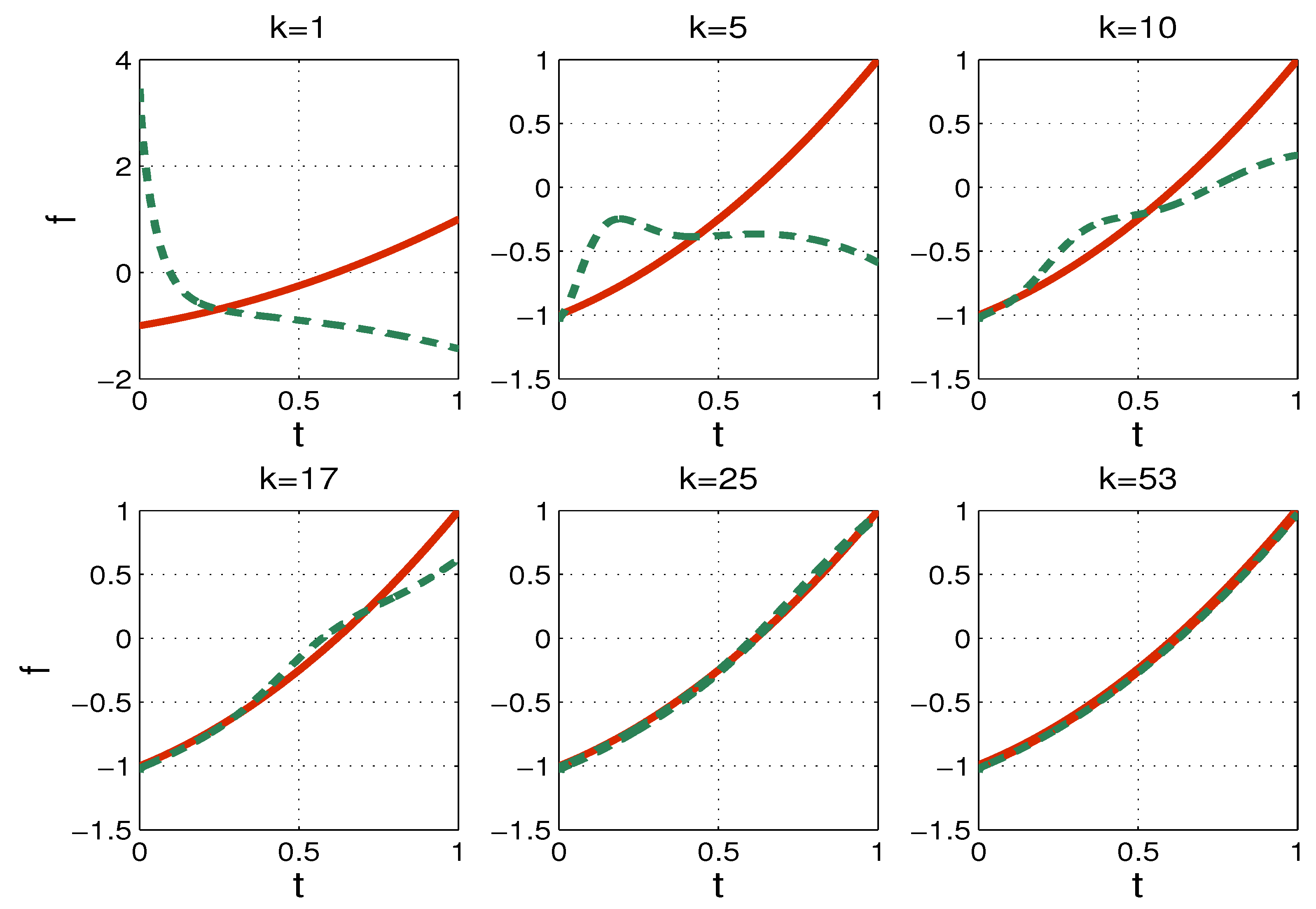
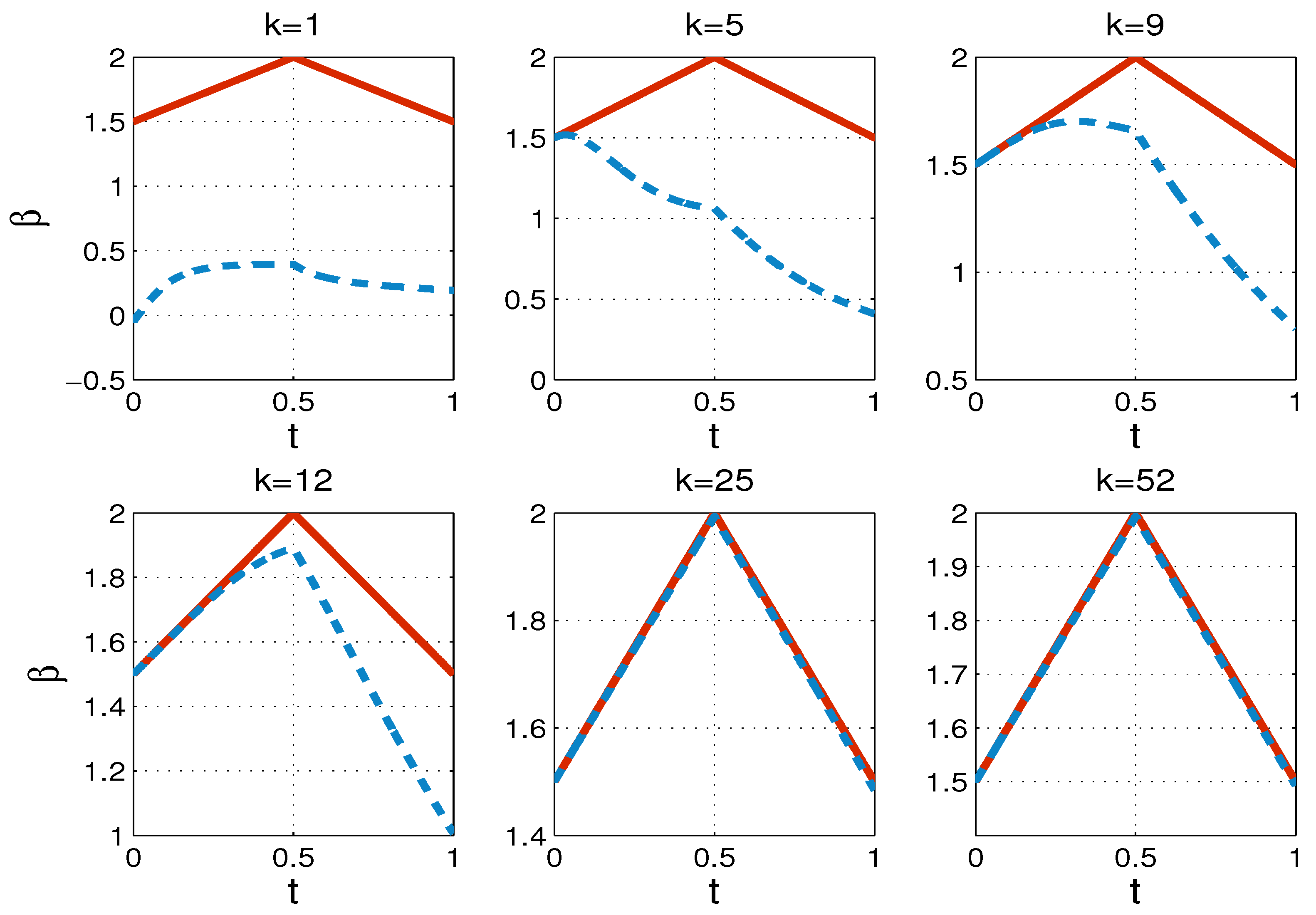
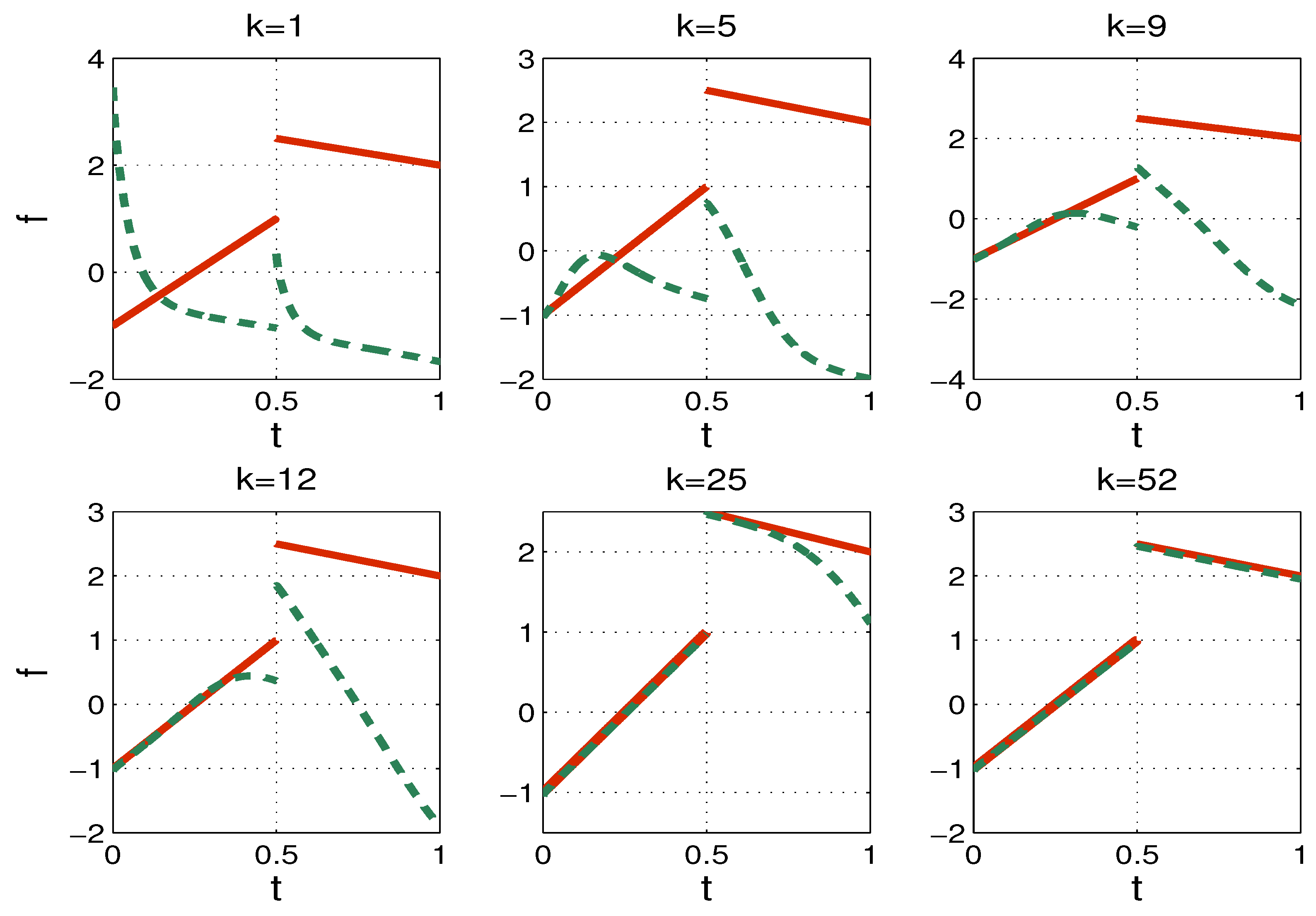
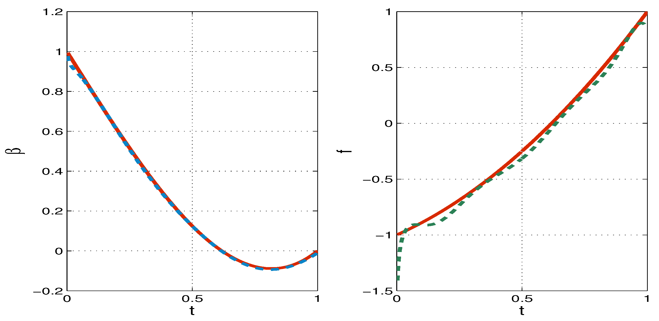
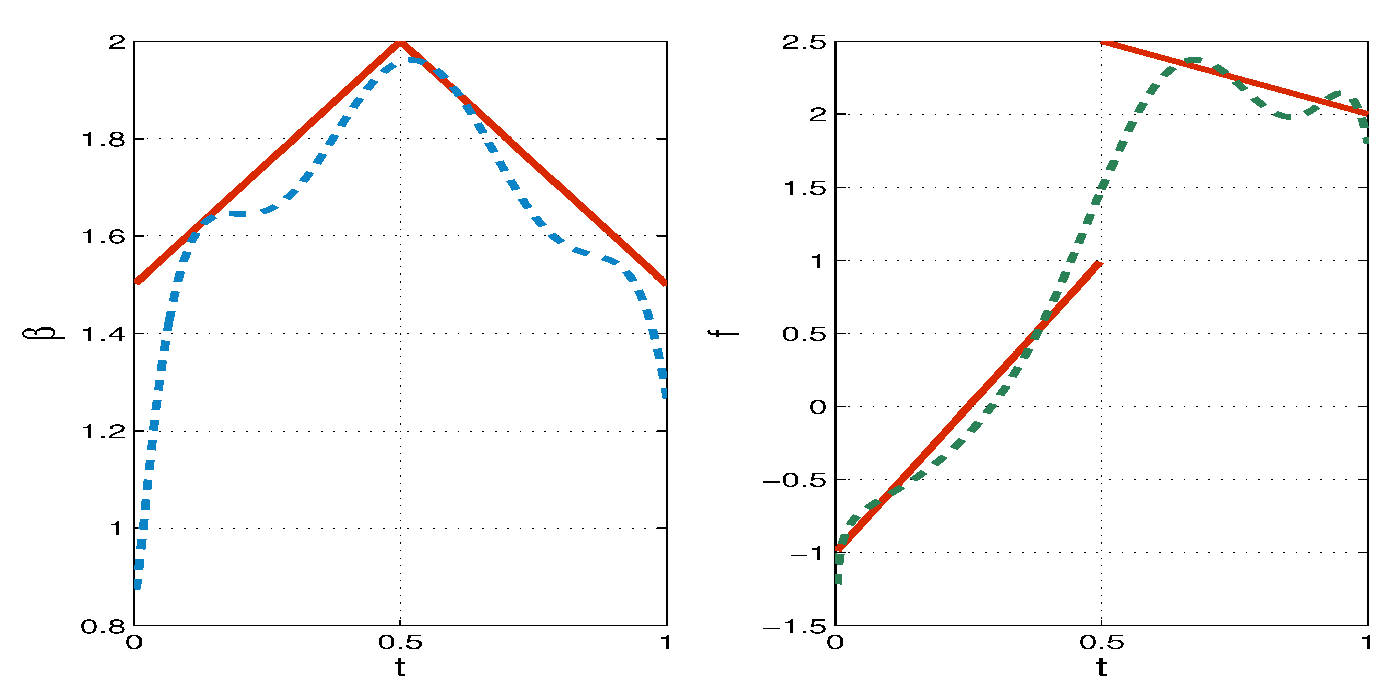
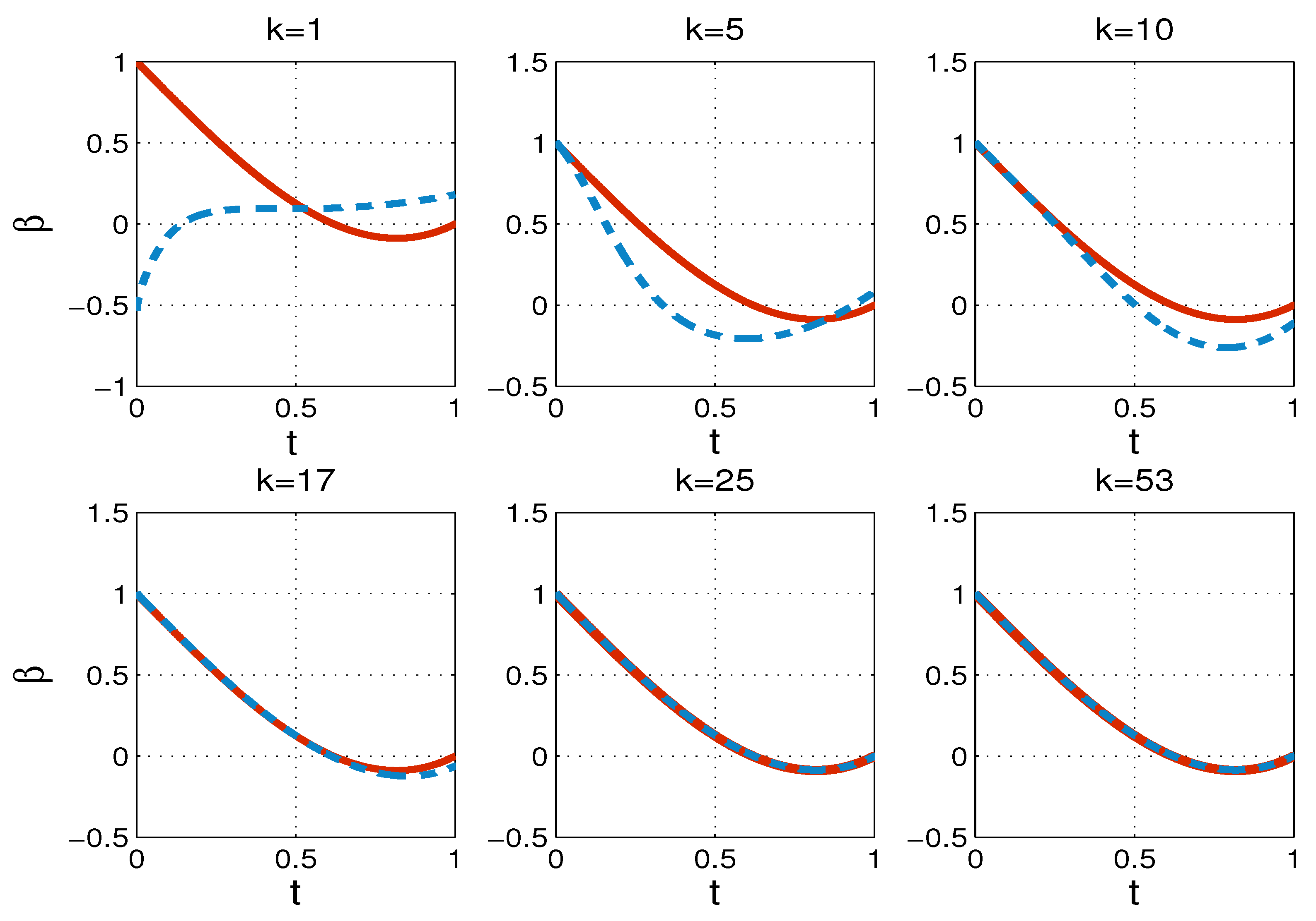
First, we illustrate the recovering process of functions β and f. In Figure 1 and Figure 2, we plot the exact and restored function, β and f, respectively at different iterations k for TP1. The results for TP2 are depicted in Figure 3 and Figure 4. The computations are performed on the mesh with $N=40$ spatial grid nodes and time step $\tau =h^2$. For both examples, the convergence is achieved in 52–53 iterations. The method is not restricted by the size of the convergence range of the initial data.

Figure 1. Exact (solid line) and recovered functions $\beta$ (dashed line) at different iterations k, TP1, $N=40$, $\tau =h^2$, Example 1.

Figure 2. Exact (solid line) and recovered function f (dashed line) at different iterations k, TP1, $N=40$, $\tau =h^2$, Example 1.

Figure 3. Exact (solid line) and recovered functions $\beta$ (dashed line) at different iterations k, TP2, $N=40$, $\tau =h^2$, Example 1.

Figure 4. Exact (solid line) and recovered function f (dashed line) at different iterations k, TP2, $N=40$, $\tau =h^2$, Example 1.

In Table 1, we provide the errors and order of convergence of the numerical solution of the inverse problem for different numbers of space grid nodes N and fixed $\tau =h^2$. We observe that the spatial order of convergence both for TP1 and TP2 is secondary.

Table 1. Errors and convergence rate of the numerical solutions $u^h$ and $B^h$ of the inverse problem, Example 1.

	TP1				TP2
$\mathbf{N}$	${\mathcal{E}}_{\mathit{u}}$	${\mathcal{CR}}_{\mathit{u}}$	${\mathcal{E}}_{\mathit{B}}$	${\mathcal{CR}}_{\mathit{B}}$	${\mathcal{E}}_{\mathit{u}}$	${\mathcal{CR}}_{\mathit{U}}$	${\mathcal{E}}_{\mathit{b}}$	${\mathcal{CR}}_{\mathit{b}}$
20	$4.7178\times {10}^{-3}$		3.4785 $\times {10}^{-3}$		$1.3368\times {10}^{-2}$		$8.2245\times {10}^{-3}$
40	$1.2236\times {10}^{-3}$	1.9470	$8.9581\times {10}^{-4}$	1.9572	$3.5848\times {10}^{-3}$	1.8988	$2.2157\times {10}^{-3}$	1.8921
80	$3.1005\times {10}^{-4}$	1.9805	$2.2663\times {10}^{-4}$	1.9829	$9.2213\times {10}^{-4}$	1.9589	5.7206 $\times {10}^{-4}$	1.9535
160	$7.7300\times {10}^{-5}$	2.0040	$5.6944\times {10}^{-5}$	1.9927	$2.3260\times {10}^{-4}$	1.9871	1.4507 $\times {10}^{-4}$	1.9794
320	$1.9307\times {10}^{-5}$	2.0013	$1.4242\times {10}^{-5}$	1.9994	$5.7585\times {10}^{-5}$	2.0141	$3.6478\times {10}^{-5}$	1.9916

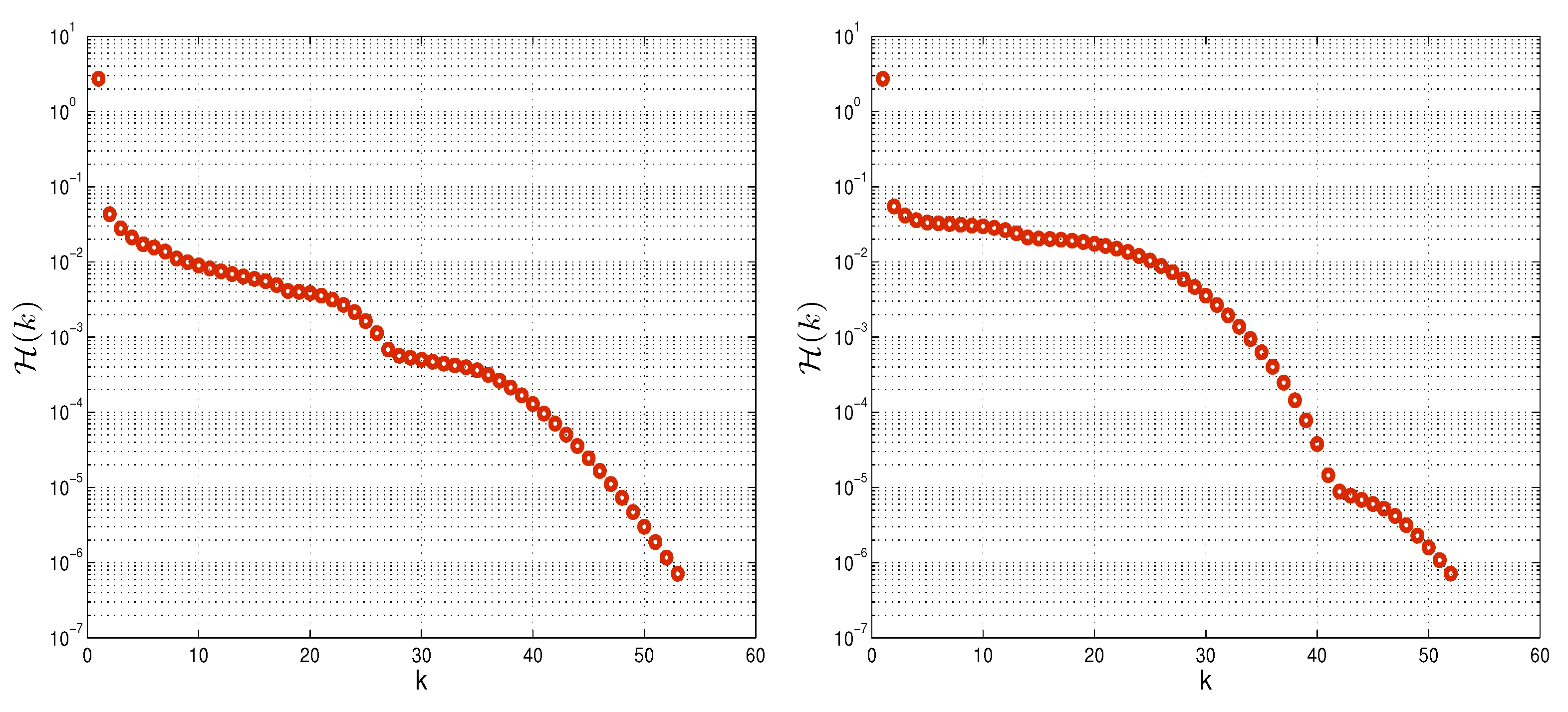
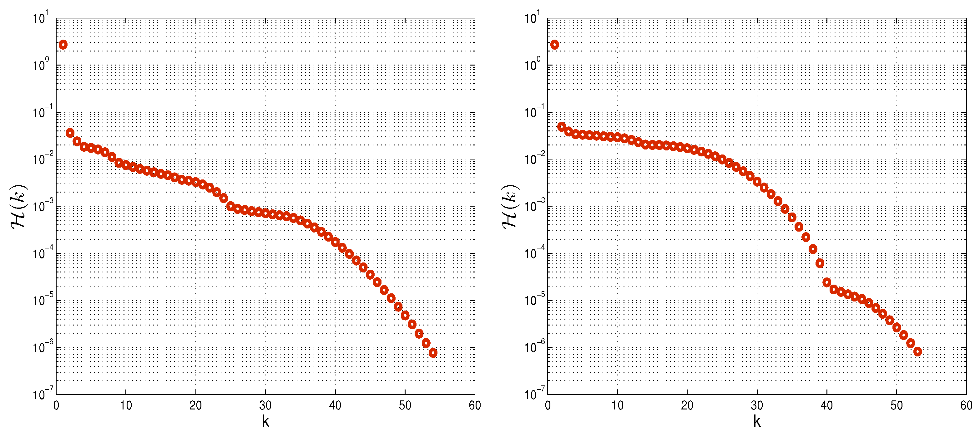
In Figure 5, we show the convergence of the iteration processes for TP1 and TP2. The iteration process is efficient at recovering smooth and non-smooth and discontinuous functions.

Figure 5. $\mathcal{H}\left(k\right)$ at each iteration, TP 1 (left), TP2 (right), $N=40$, $\tau =h^2$, Example 1.

Example 2 

(Noisy data). Now, we deal with perturbed measurements, generated as follows

$$E^{\sigma }\left(t_n\right)=E\left(t_n\right)+2{\sigma }_{1}E\left(t_n\right)({\rho }_1\left(t_n\right)-0.5),F^{\sigma }\left(t_n\right)=F\left(t_n\right)+2{\sigma }_{2}E\left(t_n\right)({\rho }_2\left(t_n\right)-0.5),$$

where $E\left(t_n\right)$, $F\left(t_n\right)$ are obtained as in Example 1, ${\sigma }_1$, ${\sigma }_2$ are noise levels and ${\rho }_1\left(t_n\right)$, ${\rho }_2\left(t_n\right)$ are a random vectors uniformly distributed at an interval of $[0,1]$. Then, we smooth the data using a polynomial curve fitting of 7 degrees.

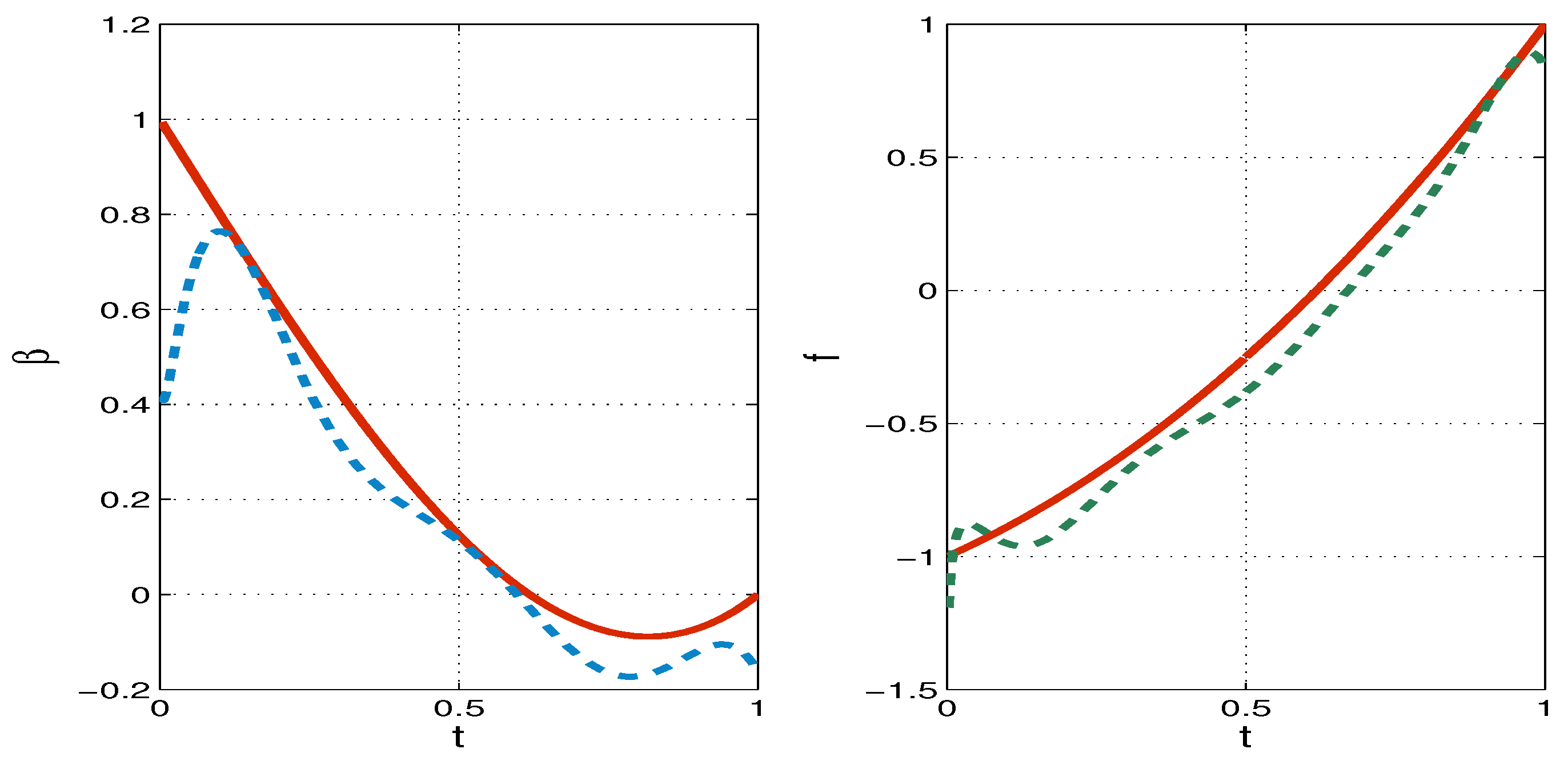
All of the computations are performed for $N=320$ and $\tau =h$. In Figure 6, we plot the exact and recovered functions determined by Algorithm 1, using functions β and f for TP1, ${\sigma }_1=0.003$, ${\sigma }_2=0.002$. In this case, ${\mathcal{E}}_U=4.3647\times {10}^{-3}$, ${\mathcal{E}}_b=1.6098\times {10}^{-3}$ and the accuracy ϵ is obtained at $k=54$ iterations. In Figure 7, we illustrate the recovery in the case of bigger noise. The errors of the numerical solutions are ${\mathcal{E}}_U=1.4443\times {10}^{-2}$, ${\mathcal{E}}_b=2.4217\times {10}^{-2}$ and $k=54$. In Figure 8, we depict exact recovered functions of β and f for TP2, ${\sigma }_1=0.01$, ${\sigma }_2=0.03$. In this case, $k=53$ and ${\mathcal{E}}_U=2.6049\times {10}^{-2}$, ${\mathcal{E}}_b=2.9370\times {10}^{-2}$. Note that the number of iterations required to reach the error tolerance ϵ is only slightly increased compared with the noise-free data test. This can also be seen in Figure 9, where the convergence of the iteration processes for both TP1and TP2 is shown.

Figure 6. Exact (solid line) and recovered (dashed line) functions $\beta$ (left) and f (right), TP1, ${\sigma }_1=0.003$, ${\sigma }_2=0.002$, Example 2.

Figure 7. Exact (solid line) and recovered (dashed line) functions $\beta$ (left) and f (right), TP1, ${\sigma }_1=0.01$, ${\sigma }_2=0.03$, Example 2.

Figure 8. Exact (solid line) and recovered (dashed line) functions $\beta$ (left) and f (right), TP2, ${\sigma }_1=0.01$, ${\sigma }_2=0.03$, Example 2.

Figure 9. $\mathcal{H}\left(k\right)$ at each iteration, TP 1 (left), TP2 (right), ${\sigma }_1=0.01$, ${\sigma }_2=0.03$, Example 2.

Evolution graphics of the numerical solution U and b, restored by the inverse problem and the corresponding absolute errors, are shown in Figure 10 for TP2, ${\sigma }_1=0.01$, ${\sigma }_2=0.03$.

Figure 10. Numerical solutions $u^h$ and $B^h$ in the whole computational domain, restored by the inverse problem and the corresponding absolute errors, TP2, ${\sigma }_1=0.01$, ${\sigma }_2=0.03$, Example 2.

In the case of noisy measurements, the fitting of functions $\beta$ and f, for TP1 and TP2, are sufficiently accurate, such that to obtain optimal precision of the numerical solutions U and b.

7. Conclusions

In this article, we study the inverse problem of recovering a time-dependent convection coefficient and a time-dependent source in a 1D MHD flow model on the basis of two integral observations of the solutions.

• We transform the inverse problem to a non-classical system of parabolic equations, which involve the boundary values of the solution in the differential operators.
• We show the equivalence of the obtained forward problem with the inverse problem.
• Applying the Galerkin approximation, we prove the well-posedness of the non-classical forward problem.
• An iteration algorithm, based on the FEM method, is developed for numerical solution of the inverse problems.
• The iteration process is convergent for a moderate number of iterations.
• The reconstruction of the source and convection coefficients is successful in the case when they are smooth functions, as well as for non-smooth and discontinuous functions.
• For noise-free data, the order of convergence of the numerical solution of the inverse problem is first in time and second in space.
• For the noisy measurements, the adjustment of the convection coefficient and source is accurate enough to obtain optimal precision of the numerical solutions U and b.
• The method is not limited with respect to the size of the convergence range of the initial data.
• The proposed numerical approach can also be applied in the case when the integral measurements are in the spatial subinterval.
• Galerkin approximation method, developed in this work, can be expanded to the case of the second and third kind of boundary conditions [34].

References

- He, Y. Unconditional convergence of the Euler semi-implicit scheme for the threedimensional incompressible MHD equations. IMA J. Numer. Anal. 2015, 33, 767–801. [Google Scholar] [CrossRef]
- Landav, L.D.; Bell, J.; Kearsley, M.; Pitaevski, L.; Lifshitz, E.; Sykes, J. Electrodynamics of Continuous Media; Elsevier: Amsterdam, The Netherlands, 2013. [Google Scholar]
- Ren, Z.; Guo, S.; Li, Z.; Wu, Z. Adjoint-based parameter and state estimation in 1-D magnetohydrodynamics (MHD) flow system. J. Optim. Manag. Optim. 2018, 14, 1579–1594. [Google Scholar] [CrossRef]
- Tsyba, V.; Chibatorev, A.Y. Optimal control asymptotics of a magnetohydrodynamic flow. Comp. Math. Math. Phys. 2009, 49, 466–473. [Google Scholar] [CrossRef]
- Yu, P.X.; Tian, Z.F. Comparison of the simplified and full MHD models for laminar incompressible flow past a circular cylinder. Appl. Math. Model. 2017, 41, 143–163. [Google Scholar] [CrossRef]
- Barnothy, M.F. Biological Effects of Magnetic Fields; Springer Science +Business Media, LLC: Berlin/Heidelberg, Germany, 1964. [Google Scholar]
- Yamagishi, A. Biological systems in high magnetic field. J. Magn. Arid. Magn. Mater. 1990, 90–91, 43–46. [Google Scholar] [CrossRef]
- Misra, J.; Sinha, A.; Shit, G. A numerical model for the magnetohydrodynamic flow of blood in a porous channel. J. Mech. Med. Biol. 2011, 11, 547–562. [Google Scholar] [CrossRef]
- Rashidi, S.; Esfahani, J.A.; Maskaniyan, M. Applications of magnetohydrodynamics in biological systems-a review on the numerical studies. J. Magn. Magn. Mater. 2017, 439, 358–372. [Google Scholar] [CrossRef]
- Ma, M.; Lin, B.-L.; Chen, C.; Horiguchi, F.; Eriguchi, T.; Li, Y.; Wang, X. A 3D-hydrodynamic model for predicting the environmental fate of chemical pollutants in Xiamen Bay, southeast China. Environ. Pollut. 2020, 256, 113000. [Google Scholar] [CrossRef] [PubMed]
- Bátkai, A.; Csomós, P.; Faragó, I.; Horányi, A.; Szépszé, G. Mathematical Problems in Meteorological Modelling, 1st ed.; Series Mathematics in Industry; Springer: Cham, Switzerland, 2016; 264p. [Google Scholar]
- Prusov, V.A.; Doroshenko, A.Y. Hydrodynamic modeling of industrial pollutants spreading in atmosphere. In Mathematical Problems in Meteorological Modelling Conference Proceedings; Bátkai, A., Csomós, P., Faragó, I., Horányi, A., Szépszó, G., Eds.; Springer: Cham, Switzerland, 2016; Volume 24, pp. 87–116. [Google Scholar]
- Mirparizi, M.; Zhang, C.; Amiri, M.J. One-dimensional electro-magneto-poro-thermoelastic wave propagation in a functionally graded medium with energy dissipation. Phys. Scr. 2022, 97, 045203. [Google Scholar] [CrossRef]
- Mirparizi, M.; Shariyat, M.; Fotuhi, A.R. A novel approach for generalized Green-Naghdi-type electro-magneto-thermo-hyperelasticity wave propagation and reflection investigations in near-incompressible layers under shock loads. J. Therm. Stress. 2024, 47, 743–765. [Google Scholar] [CrossRef]
- Kandilarov, J.; Vulkov, L. Simultaneous numerical reconstruction of time-dependent convection coefficient and source in magnetohydrodynamics flow system. In Studies in Computational Intelligence; Springer: Berlin/Heidelberg, Germany, 2024. [Google Scholar]
- Khankishiyev, Z.F. Solution of one problem for linear loaded parabolic type differential equation with integral conditions. Adv. Math. Model. Appl. 2022, 7, 178–190. [Google Scholar]
- Ashyralyev, A.; Emharab, F. A note on the time identification nonlocal problem. Adv. Math. Model. Appl. 2022, 7, 105–120. [Google Scholar]
- Cai, K.; Lesnic, D. Determination of time-dependent effective ion collision frequency from an integral observation. J. Inverse Ill-Posed Probl. 2024. [Google Scholar] [CrossRef]
- Georgiev, S.G. Numerical and analytical computation of the implied volatility from option price measurementsunder regime-switching. AIP Proc. 2019, 2172, 070007. [Google Scholar]
- Ashyralyev, A.; Sazaklioglu, A.U. Integration of a time-dependent source identification inverse problem with integral overdetermination. Numer. Funct. Anal. Optim. 2017, 38, 1276–1294. [Google Scholar] [CrossRef]
- Glotov, D.; Hames, W.E.; Meir, A.J.; Ngoma, S. An inverse diffusion coefficient problem for aparabolic equation with integral constraint. Int. J. Numer. Anal. Model. 2018, 15, 552–563. [Google Scholar]
- Hasanov, A.H.; Romanov, V.G. Introduction to Inverse Problems for Differential Equations, 1st ed.; Springer: Cham, Switzerland, 2017; 261p. [Google Scholar]
- Isakov, V. Inverse Problems for Partial Differential Equations, 3rd ed.; Springer: Cham, Switzerland, 2017; p. 406. [Google Scholar]
- Kabanikhin, S.I. Inverse and Ill-Posed Problems; DeGruyer: Berlin, Germany, 2011. [Google Scholar]
- Lesnic, D. Inverse Problems with Applications in Science and Engineering; CRC Press: Abingdon, UK, 2021; p. 349. [Google Scholar]
- Prilepko, A.I.; Orlovsky, D.G.; Vasin, I.A. Methods for Solving Inverse Problems in Mathematical Physics; Marcel Dekker: New York, NY, USA, 2000. [Google Scholar]
- Samarskii, A.A.; Vabishchevich, P.N. Numerical Methods for Solving Inverse Problems in Mathematical Physics; de Gruyter: Berlin, Germany, 2007; 438p. [Google Scholar]
- Vabishchevich, P.N.; Klibanov, M.V. Numerical identification of the leading coefficient of a parabolic equation. Diff. Equ. 2016, 52, 855–862. [Google Scholar] [CrossRef]
- Evans, L.C. Partial Differential Equations, 2nd ed.; Graduate Studies in Mathematics 19; American Mathematical Society: Providence, RI, USA, 2010. [Google Scholar]
- Ladyženskaja, O.A.; Solonnikov, V.A.; Ural’ceva, N.N. Linear and Quasi-Linear Equations of Parabolic Type; Translations of Mathematical Monographs 23; American Mathematical Society: Providence, RI, USA, 1988; 648p. [Google Scholar]
- Borzi, A. Modelling with Ordinarty Differential Equations, A Comprehensive Approach; Chapman and Hall/CRC: Boca Raton, FL, USA, 2020. [Google Scholar]
- Larsson, S.; Thomée, V. Partial Differential Equations with Numerical Methods; Springer: Berlin/Heidelberg, Germany, 2003. [Google Scholar]
- Thomée, V. Galerkin Finite Element Methods for Parabolic Problems, 2nd ed.; Ser. Comput. Math. 25; Springer: Berlin/Heidelberg, Germany, 2005. [Google Scholar]
- Faragó, I.; Korotov, S.; Neittaanmäki, P. Galerkin approximations for the linear parabolic equation with the third boundary condition. Appl. Math. 2003, 48, 111–128. [Google Scholar] [CrossRef][Green Version]
Disclaimer/Publisher’s Note: The statements, opinions and data contained in all publications are solely those of the individual author(s) and contributor(s) and not of MDPI and/or the editor(s). MDPI and/or the editor(s) disclaim responsibility for any injury to people or property resulting from any ideas, methods, instructions or products referred to in the content. |
© 2024 by the authors. Licensee MDPI, Basel, Switzerland. This article is an open access article distributed under the terms and conditions of the Creative Commons Attribution (CC BY) license (https://creativecommons.org/licenses/by/4.0/).