XGBoost-Enhanced Graph Neural Networks: A New Architecture for Heterogeneous Tabular Data

Abstract

Graph neural networks (GNNs) perform well in text analysis tasks. Their unique structure allows them to capture complex patterns and dependencies in text, making them ideal for processing natural language tasks. At the same time, XGBoost (version 1.6.2.) outperforms other machine learning methods on heterogeneous tabular data. However, traditional graph neural networks mainly study isomorphic and sparse data features. Therefore, when dealing with tabular data, traditional graph neural networks encounter challenges such as data structure mismatch, feature selection, and processing difficulties. To solve these problems, we propose a novel architecture, XGNN, which combines the advantages of XGBoost and GNNs to deal with heterogeneous features and graph structures. In this paper, we use GAT for our graph neural network model. We can train XGBoost and GNN end-to-end to fit and adjust the new tree in XGBoost based on the gradient information from the GNN. Extensive experiments on node prediction and node classification tasks demonstrate that the performance of our proposed new model is significantly improved for both prediction and classification tasks and performs particularly well on heterogeneous tabular data.

1. Introduction

As AI becomes more prevalent in many real-world applications, tabular data storage is becoming more common. A table format organizes tabular data. It is also commonly known as structured data. Tabular data are a commonly used data type in various fields, including medicine [1], finance [2], online advertising [3], and recommender systems [4]. They usually consist of rows and columns, where each row represents a data instance, and each column represents a feature or attribute. Columns in tabular data can contain different types of data, including numeric, categorical, textual, date-time, etc. Tables can mix these different data types.

In recent years, with the rapid development of deep learning in text, image, and audio, people have started to show great interest in its application to tabular data. However, the effectiveness of deep learning when working with tabular data is largely dependent on the homogeneity of the input data, as well as the fact that the structure used to organize the information provides insight into the data. Deep learning performs better on tabular data only when these conditions are met. Integrated tree-based models, such as GBDT [5], XGBoost [6], CatBoost [7], and LightGBM [8], have achieved state-of-the-art SOTA on tabular data, excelling in competitive prediction accuracy and fast training speed. However, tree-based methods also have limitations in some specific scenarios, such as in the case of continuous learning or reinforcement learning, when the tabular data are only a part of the model input or when the tabular data also include information such as images, text, or audio. In these cases, it is necessary to consider other methods, such as graph neural networks (GNNs), which do not depend on the order of nodes but also take into account both the neighborhood information of the nodes and the node features for prediction.

The following key attributes and features of XGBoost contribute to its success when handling tabular data: (1) Automatic handling of missing values. When splitting nodes, XGBoost seeks the optimal method to fill in the missing values, ensuring the model’s performance remains unaffected. (2) Feature importance scoring. It helps users understand which features contribute most to model prediction. This is useful for feature selection and model interpretation. (3) Regularization. Additionally, the model uses a gradient boosting framework and L1 and L2 regularization to effectively avoid overfitting and improve its generalization abilities. (4) Gradient enhancement framework. We utilize an optimized tree structure to facilitate efficient model training and prediction, thereby enhancing overall performance. In contrast, a key feature of GNN is its ability to directly process graph-structured data, effectively capturing and utilizing the relationships between nodes and edges in graph-structured data. XGBoost primarily handles tabular data, unlike GNNs. A GNN requires converting textual data into graph structures, such as word co-occurrence graphs, dependent syntactic graphs, or semantic graphs, rather than using raw tabular data directly. Although this preprocessing differs from XGBoost’s feature engineering, it is also a critical step for the algorithm’s success.

It goes without saying that both the XGBoost and GNN methods have their own benefits. Is it possible to combine the benefits of both models? The current work is the first to use the XGBoost model for graph-structured data on text categorization and prediction tasks, to the best of our knowledge. In this paper, we propose a new architecture, XGNN—a joint training of XGBoost and GNN models. It is possible to achieve end-to-end optimization by using XGBoost’s heterogeneous feature processing and GNN’s graph structure processing. This makes the model work better overall. Here is a summary of our contributions:

(1)

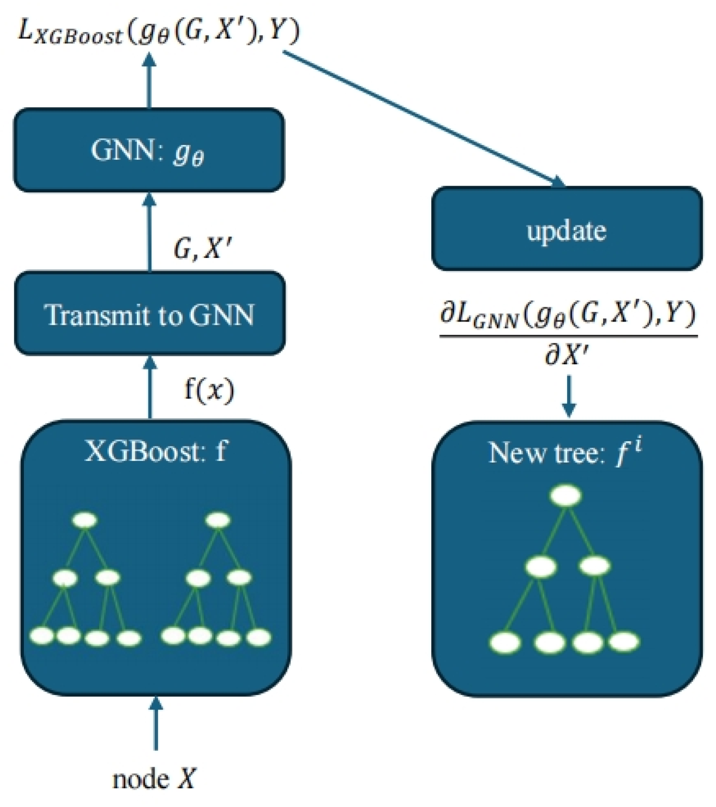
We introduce XGNN, a graph neural network model for tabular data, to jointly train the XGBoost and GNN models. We believe this is the first time we have jointly studied these two models in the field of tabular data.

(2)

The dataset types chosen in this paper are rich, including heterogeneous datasets, isomorphic datasets, sparse datasets, and bag-of-words datasets, which are involved in binary classification and multi-classification problems. We simultaneously achieve good results in both node prediction and node classification tasks.

(3)

We also investigated the use of four different types of graph neural networks co-trained with XGBoost, and experiments showed that using different types of graph neural networks, XGNN can still outperform other models.

The paper begins with an introduction of the research background; Section 2 presents the related work on tabular models for three categories; and Section 3 describes the proposed new model—the XGNN. Section 4 describes the dataset used in this paper, the baseline model, the experimental parameter settings, the analysis of the results, and the ablation experiments. Section 5 concludes the paper and suggests future research directions.

2. Related Work

2.1. Tree-Based Table Model

Tree-based tabular integration models, including GBDT, XGBoost, CatBoost, and LightGBM, are one of the more popular methods for processing tabular data nowadays. Bentéjac et al. [5] combine multiple weak learners, usually decision trees, to create strong learners. The main principle of GBDT is to construct a series of weak learners step by step, and each of them adjusts its prediction based on the residuals (prediction errors) of the previous round to adjust the predictions, thus gradually improving the model’s performance. In a variety of machine learning and data science tasks, Sagi et al. [6] proposed the machine learning algorithm XGBoost, a decision tree ensemble algorithm based on the gradient boosting principle. Prokhorenkova et al. [7] made an improvement algorithm for classification and regression trees that uses the gradient boosting principle. This resolved the issue of prediction bias resulting from special target leakage. Ke et al. [8] proposed LightGBM, including two new techniques: gradient-based unilateral sampling (GOSS) and exclusive feature bundling (EFB). They say that it speeds up traditional GBDT training by more than 20 times while maintaining almost the same accuracy. However, why do tree-based models still outperform deep learning on tabular data? When dealing with non-smooth functions or decision boundaries, tree-based tabular models can identify sharp points in the search space as well as some random functions [9]. Additionally, they are capable of discerning the usefulness of features and avoiding those that are unnecessary in order to select the optimal path. When dealing with rotated data sets, tree models do not have local invariance, which makes them better able to handle tabular data without properties.

2.2. Deep Learning-Based Table Models

With deep learning’s success in tasks involving text, sound, or images, research has begun to investigate the best way to apply these models to tabular data. Popov et al. [10] developed Neural Oblivious Decision Integration (NODE), a differentiable deep GBDT that underwent backpropagation training from start to finish. This was carried out for deep learning on different types of tabular data. Ke et al. [11] proposed TabNN to automatically derive effective neural network architectures for tabular data in various tasks. The design of TabNN follows two principles: explicit utilization of expressive feature combinations and reduction of model complexity. Paliwal et al. [12] proposed TableNet, which processes tabular images by convolutional neural networks (CNNs) and generates predictions of tabular regions, cells, rows, columns, etc. Prasad et al. [13] created the CascadeTabNet cascade model. This model uses a faster R-CNN to find table regions, followed by separate models for recognizing table rows and columns. While deep learning methods perform well on classification or data generation tasks on isomorphic data (e.g., image, audio, and text data), handling tabular data is still a challenge for deep learning models. Tabular data are heterogeneous, with dense numerical features and sparse categorization features compared to image or linguistic data, and the correlation between features is relatively weak.

2.3. Tabular Model Based on Graph Neural Network

Graph neural networks have generated discussion in the field of tabular data learning by virtue of their inherent ability to model complex relationships and interactions between different elements of tabular data. Guo et al. [14] proposed TabGNN, which learns multifaceted sample relationships and enhances sample representations by constructing multiplexed graphs and multiplexed graph neural networks. Telyatnikov et al. [15] proposed EGG-GAE, a novel EdGe generative graph autoencoder for missing data interpolation, which processes randomly sampled small batches of input data and automatically infers the optimal connectivity of each architectural layer in small batches. Du et al. [16] introduced TabularNet, a WordNet tree-based neural network architecture that utilizes row- and column-level pooling and bi-directionally gated recurrent units (Bi-GRUs) to capture statistics and local positional correlations. Liao et al. [17] describe TabGSL, a new way to improve tabular data prediction by learning both instance correlation and feature interaction at the same time in a single framework. The advantage of graph neural networks in tabular models is that they can effectively capture the complex relationships between entities in a table and improve the model’s ability to understand structured data. However, training and inference for large-scale tabular data come with a high computational cost, and we must also overcome the challenges posed by data sparsity and incompleteness.

In general, for node classification and node prediction on tabular data, deep learning-based tabular models lack the ability to understand and process the inherent structure of tables. Tree-based models and graph neural network-based models, on the other hand, are better at capturing tabular data’s hierarchical structure and complex relationships between nodes. That is why we chose to combine these two models to make node prediction and classification tasks more accurate.

3. Models and Methods

Although the gradient enhancement-based approach is successful for learning tabular data, it has technical difficulties in graph-structured data applications. For example, how do you effectively integrate the relational information between data points into traditional tabular data models? How can we jointly train XGBoost and GNN? For the first problem, our scheme is to transform the tabular data into a graph structure, in which each data point serves as a node and the relationships between nodes serve as edges. If the data points have time–series relationships, we can define edges based on specific relationship signals, such as measuring the similarity between two data points by distance or similarity and constructing edges based on temporal order. For the second problem, our approach involves conducting comparative experiments, specifically Res-GNN, in which we directly train the node features on the XGBoost model. We then use these predictions to create new node features in the GNN, incorporating the initial inputs. However, the XGBoost model completely ignores the graph structure and misses some of the graph features, resulting in a failure to provide correct input information. XGNN, on the other hand, trains both XGBoost and GNN simultaneously, iteratively updating the XGBoost model by adding new trees that approximate the GNN loss function, as depicted in Figure 1.

Figure 1. Training of XGNN.

Algorithm 1 outlines of the XGNN training process.

Algorithm 1 Training of XGNN

1.    Input: Graph G, node features X, targets Y

2.    Initialize XGBoost targets y = Y

3.    for epoch i = 1 to N do

4.         # Train m trees of XGBoosts with Equations (2) and (3)

5.          ${f^i\leftarrow arg minL}_{\mathrm{X}\mathrm{G}\mathrm{B}\mathrm{o}\mathrm{o}\mathrm{s}\mathrm{t}}(f^i(\mathrm{X}),\widehat{\mathcal{Y}})$

6.                 $f\leftarrow f^i+f$

7.         # Train l steps of GNN

8.         ${\mathrm{X}}^{\prime }\leftarrow f(\mathrm{X})$

9.          ${{\mathrm{X}}^{\prime }\leftarrow arg minL}_{\mathrm{G}\mathrm{N}\mathrm{N}}(g_{\theta }(G,{\mathrm{X}}^{\prime }),Y)$

10.         # Update targets for next iteration of XGBoosts

11.              $y\leftarrow {\mathrm{X}}^{\prime }\leftarrow f(\mathrm{X})$

12.    end for

13.    Output: Models XGBoost f and GNN gθ

In Algorithm 1, we suggest a new XGNN model that combines the best features of XGBoost and graph neural networks (GNNs). Its goal is to quickly solve prediction problems at the node level, such as semi-supervised node regression and classification tasks. The first inputs are graph G, node features X, and target Y. In the first iteration, by minimizing the loss function $L_{\mathrm{X}\mathrm{G}\mathrm{B}\mathrm{o}\mathrm{o}\mathrm{s}\mathrm{t}}(f^i(\mathrm{X}),\widehat{\mathcal{Y}})$, we construct the XGBoost model, which contains m decision trees $f^1(\mathrm{x})$. RMSE, or cross entropy of classification, is averaged over the training set using Equations (1) and (2), where $f^{t-1}$ the model was constructed after the previous iteration, and $g^t$ is the weak learner.

$$f^t(\mathrm{x})=f^{t-1}(\mathrm{x})+ϵg^t(\mathrm{x}),$$

(1)

$$g^t=\underset{h\in \mathcal{H}}{\arg min}{\sum }_i(-\frac{\partial L(f^{t-1}({\mathrm{x}}_i),y_i)}{\partial f^{t-1}({\mathrm{x}}_i)}-g({\mathrm{x}}_i){)}^2,$$

(2)

Next, we update the node feature ${\mathrm{X}}^{\prime }$ based on the prediction of f¹ (x) and feed it to the GNN. We minimize the graph neural network based on graph G by reducing its loss function of the $g_{\theta }$. The node features of the GNN are subjected to $l$ round gradient descent optimization, thus optimizing the parameters of the GNN $\theta$ and node features ${\mathrm{X}}^{\prime }$. Using Equation (3), we define the optimized node feature ${\mathrm{X}}_{\mathrm{new} }^{\prime }$ difference is the difference with the original input feature ${\mathrm{X}}^{\prime }=f^1(\mathrm{X})$ difference, which serves as the objective of XGBoost new tree construction, where $\eta$ the learning rate is determined.

$${\mathrm{X}}_{\mathrm{new} }^{\prime }={\mathrm{X}}^{\prime }-\eta \frac{\partial L_{\mathrm{G}\mathrm{N}\mathrm{N}}(g_{\theta }(G,{\mathrm{X}}^{\prime }),Y)}{\partial {\mathrm{X}}^{\prime }},$$

(3)

Finally, in the second iteration, the predictions $f(\mathrm{X})=f^1(\mathrm{X})+f^2(\mathrm{X})$ are summed and the updated ${\mathrm{X}}^{\prime }$ is passed to the GNN again, and the GNN model again performs the $l$ step of direction propagation and takes the new difference ${\mathrm{X}}_{\mathrm{new} }^{\prime }-{\mathrm{X}}^{\prime }$ as the target of the next XGBoost, and so on. The model outputs the XGNN model after N rounds of training.

3.1. Extreme Gradient Boosting (XGBoost)

XGBoost is an efficient gradient boosting decision tree algorithm based on GBDT (gradient boosting decision tree), which is based on the model of a boosting algorithm. Boosting is the process of accumulating the weak learners generated at each time and weighting them to the total model to form a strong learner, which can be used for regression and classification problems. The basic idea of XGBoost is the same as GBDT but optimized in these aspects, including second-order derivatives to make the loss function more accurate, regular terms to avoid tree overfitting, block storage that can be computed in parallel, and so on. Firstly, the objective function is defined as Equation (4); Equation (5) is the Taylor expansion; Equation (6) is the complexity of a tree; and Equation (7) is the definition of a tree.

$$\mathrm{obj}\left(\theta \right)={\sum }_i^{n}l\left(y_i,\widehat{y_i}\right)+{\sum }_{k=1}^K\mathsf{\Omega }\left(f_k\right),$$

(4)

$${\sum }_{i=1}^n[g_i{f}_t(x_i)+\frac{1}{2}{h}_i{f}_t^2(x_i)]+\mathsf{\Omega }(f_t),$$

(5)

$$\mathsf{\Omega }(f_t)=\gamma T+\frac{1}{2}\lambda {\sum }_{j=1}^T{w}_j^2,$$

(6)

$$f_t(x)=w_{q(x)},w\in R^T,q:R^d\to \{\mathrm{1,2},\cdots ,T\},$$

(7)

where $K$ denotes the number of trees, and $f$ denotes the function space $F$ in which a function representing an abstract structure like a tree. $l$ is our loss function, and $\mathsf{\Omega }$ is the penalty term. $g_i$ and $h_i$ are the first- and second-order derivatives of our loss function with respect to ${\widehat{yi}}^{(t-1)}$, the first- and second-order derivatives of $w$, which denotes the weight vector. $\gamma T$ is the number of leaves and $\frac{1}{2}\lambda {\sum }_{j=1}^T{w}_j^2$ is the square of the L2 module of W, and $q$ denotes the leaf node mapping relation corresponding to each data sample. At the same time, we define $R^d\to \{\mathrm{1,2},\cdots ,T\}$ to denote the set of nodes that a given sample maps to. Since multiple samples will fall into a single node, we change the scope of the definition of the objective function from n samples to T nodes.

Then, the above objective function is processed to obtain Equation (8); if the gain > 0, it means that the cut object is smaller, and the model is better.

$$\mathrm{Gain} =\frac{1}{2}[\frac{G_L^2}{H_L+\lambda }+\frac{G_R^2}{H_R+\lambda }-\frac{{(G_L+G_R)}^2}{H_L+H_R+\lambda }]-\gamma ,$$

(8)

Although XGBoost can use pre-sorting and approximation algorithms to reduce the computation when finding the optimal cut-points of leaf minima, the time overhead is still large because it needs to traverse the whole dataset. Moreover, the space complexity of pre-sorting is high, as it not only needs to store the feature values but also the indexes of the gradient statistics of the samples corresponding to the features, resulting in an exponential increase in memory consumption. The introduction of graph neural networks (GNNs) can solve these problems to some extent, especially in feature engineering and complex feature relationship processing.

3.2. Graph Neural Networks (GNNs)

Given an attribute graph G = (V, E, X), where x_i is the d-dimensional feature vector of node vi, the GNN algorithm can learn to generate a node representation for each node v_i ∈ V by implementing the aggregate function combining the function sums $g_i$. These two functions are typically iterated multiple times in each graph neural network layer in order to continuously update the node representation as information is passed. Assuming that we are training an m-layer GNN, the nodes embedded in the mth layer, i.e., $g_i(m)$, can be obtained by using Equations (9) and (10):

$${\mathrm{a}}_i^{(k)}={\mathrm{a}\mathrm{g}\mathrm{g}\mathrm{r}\mathrm{e}\mathrm{g}\mathrm{a}\mathrm{t}\mathrm{e}}^{(k)}({\mathrm{h}}_j^{(k-1)}:v_j\in \mathcal{N}(v_i)),$$

(9)

$${\mathrm{h}}_i^{(k)}={\mathrm{c}\mathrm{o}\mathrm{m}\mathrm{b}\mathrm{i}\mathrm{n}\mathrm{e}}^{(k)}({\mathrm{h}}_i^{(k-1)},{\mathrm{a}}_i^{(k)}),$$

(10)

of which $g_i(0)={\mathrm{x}}_i$, $g_i{=g}_i(m)$, the ${\mathrm{a}\mathrm{g}\mathrm{g}\mathrm{r}\mathrm{e}\mathrm{g}\mathrm{a}\mathrm{t}\mathrm{e}}^{(m)}(.)$ and ${\mathrm{c}\mathrm{o}\mathrm{m}\mathrm{b}\mathrm{i}\mathrm{n}\mathrm{e}}^{(m)}(.)$ are the aggregation and combination functions of the mth layer, respectively.

So how does the GNN learn from a graph representation? Again, in a graph G = (V, E, X) with attributes, for each node v_i ∈ V, we obtain its derived node representation g_i. By reading out the function $\mathrm{R}(.)$, the embedding of all nodes is mapped to a representation $g_G$ of the whole graph G. This readout function can be a simple permutation-invariant function, such as a summation or pooling method.

When dealing with heterogeneous graphs, traditional GNN models (e.g., GCN, GAT, APPNP, and AGNN) all require some adjustments or special designs to accommodate the diversity of nodes and edges. By introducing node-type encoding, considering edge-type information, utilizing meta-paths, designing multi-type attention modules, or employing type-aware aggregation and hybrid strategies, these models can better capture complex structures and relationships in heterogeneous graphs and improve performance on heterogeneous graphs. For processing heterogeneous data, we chose a traditional GNN model over a specially designed heterogeneous GNN model combined with XGBoost. This was done because of model complexity, data characteristics, the difficulty of combining models, computational resources and efficiency, and the ability to understand and withstand errors in the model.

3.3. Why Use GNN for TDL?

Although traditional machine learning methods perform well when dealing with tabular data, they may have limitations when it comes to nonlinear relationships, high-dimensional features, or the need to consider complex associations between features. GNN-based learning methods for tabular data have also achieved state-of-the-art status in various applications such as click-through rate prediction [18], cybersecurity [19], medical risk prediction for population health records [20], and missing data input [21]. We summarize why GNN can excel at tabular data learning in the following five areas:

(1)

Modelling instance correlation. When dealing with downstream tasks, it is necessary to consider not only the features of each instance itself but also the correlation between instances. The key idea is to learn high-quality feature representations of instances by modelling correlations between instances. If two instances have similar downstream labels, they may be closer in the feature space because they may share certain features or represent similar attributes. On the contrary, if two instances have different downstream labels, then they may be farther away from each other in the feature space because they may be significantly different from each other.

(2)

Feature interactions. In table prediction tasks, individual features may not be sufficient to adequately describe the data because there may be complex interactions between features. Traditional methods learn feature interactions by manually enumerating possible feature combinations, but this approach is time-consuming and requires domain knowledge. Deep learning methods can automatically learn feature interactions, but they usually simply connect the learned feature representations and cannot model structured correlations between features. However, GNNs can perform better in prediction tasks by learning how features interact in graph structures, naturally picking up on complex structured correlations between features, and making their own embeddings to show how features interact.

(3)

Higher-order connectivity. Higher-order connectivity refers to modelling complex relationships between data elements through the interaction of multiple hopping neighbors. To better learn the feature representation of data elements and improve prediction performance, higher-order connectivity between instances, between features, and between instances and features needs to be considered. In GNNs, through message passing and aggregation mechanisms, data elements can receive embed-dings from multi-hop neighbors in the graph to learn more complex relationships between data elements [22].

(4)

Monitoring signals. In some real-world applications, such as fraud detection, health prediction, and personalized marketing, it is challenging to collect a sufficient amount of tagged-form data. This is due to the fact that obtaining labelled data can be time-consuming and resource-intensive, often resulting in restricted access. However, graph neural networks are capable of learning without explicit instructions. This means that they can use the connections between the nodes in the graph to make better feature representations of unlabeled data, which helps with the supervised sparsity problem. We co-design the self-supervised task by combining the features and the graph structure, leveraging the semi-supervised learning property of graph neural networks. This further improves the model’s performance on the supervised sparsity problem and brings new breakthroughs in tabular data learning.

(5)

Generalization ability. GNNs can learn to generalize what they have learned from training data. This means that even if they see nodes or graph structures, they have not seen before, they can still figure out what the results should be based on the patterns they have learned from the training data. During the testing phase, they can incorporate additional features and perform feature extrapolation to learn how to represent tabular data. The ability to generalize to unseen tasks, i.e., tasks not learned during the training phase, is another crucial aspect. This implies that GNNs, when learning representations of tabular data, can apply to new, unknown tasks without requiring retraining or parameter tuning [23].

4. Experiment

4.1. Dataset

Table 1 lists five real node regression datasets with different attributes, including four heterogeneous datasets and one isomorphic dataset. California Housing [24] provides housing information and demographics of a specific area in California in 1990, with 20,640 instances and 8 numerical features commonly used in regression problems to predict property prices. We retain the following node features: median, house age, average room size, average bedroom size, population, and average occupancy percentage. County [25] contains statistical information about US counties. A node represents a county, and if two nodes share the same edge, they form a connection. We retain the following node features commonly used in regression problems to predict unemployment: DEM, GOP, Median Income, MigraRate, BirthRate, DeathRate, and BachelorRate. VK [26] is a social network dataset, and in this paper, we use the open-access sub-sample of the VK social network of the top 1 million users. The following node features are retained: country, city, followers_count, has_mobile, last_seen_time, last_seen_platform, political, languages, religion_id, alcohol, smoking, relation, sex, and university, commonly used in regression problems to predict age. Wiki [27] is a page-page network isomorphic dataset on the topic of squirrels, with retained node features being bags of informative nouns (3148 in total) appearing in the primary text of Wikipedia articles, and the task is to predict the monthly average traffic per article between October 2017 and November 2018. Avazu [28] contains records of users clicking on advertisements in mobile advertising scenarios. The node features retained are the first 100,000 rows to calculate the click-through rate per device id, filtering out ids that do not have at least 10 advertisements displayed. The nodes are characterized by the anonymity categories: C1, C14, C15, C16, C17, C18, C19, C20, and C21. It is frequently used in regression problems to predict the click-through rate per device.

Table 1. Node regression dataset.

Dataset	House	County	VK	Avazu	Wiki
#Nodes	20,640	3217	54,028	1297	5201
#Edges	182,146	12,684	213,644	54,364	198,493
#Features/Node	6	7	14	9	3148
Mean Target	2.06	5.44	35.47	0.08	27,923.76
Min Target	0.14	1.7	13.48	0	16
Max Target	5.00	24.1	118.39	1	849,131
Median Target	1.79	5	33.83	0	9225

Table 2 also lists five real-node classification datasets with different attributes. We chose the House and VK datasets from the regression task because there were not many publicly available datasets with nodes that had different properties. We then made two new datasets, House_class and VK_class, by breaking the target labels into separate classes. We also selected two sparse node classification datasets, SLAP and DBLP. SLAP [29] is constructed as a multi-hub network that connects different types of nodes through relational edges between nodes, which include a variety of associations such as gene–gene, gene–disease, and disease–compound. Regression problems commonly use it to predict which of the 15 gene types it belongs to. DBLP [30] is a multi-relational academic network dataset that includes node types such as author, paper, and conference, as well as edge relationships such as author–paper, paper–conference, and author–author. We perform various graph analysis tasks, such as node classification, link prediction, and community detection. Finally, we select an isomorphic dataset, OGB-ArXiv [31], in which each node represents a paper, and the edges signify citation relations, i.e., citations between papers. This dataset has 169,343 nodes, 1,166,243 edges, and 40 categories, making it a popular choice for classifying papers into domain categories. We preprocess the data by normalizing numerical features with a zero mean and unit variance, coding categorical features with ordinal coding, and supplementing missing values with zeros.

Table 2. Node classification dataset.

Dataset	SLAP	DBLP	OGB-ArXiv
#Nodes	20,419	14,475	169,343
#Edges	172,248	40,269	1,166,243
#Features/Node	2701	5002	128
Classes	15	4	40
Min Class	103	745	29
Max Class	534	1197	27,321

4.2. Compared Algorithms

(1)

CatBoost: A decision tree algorithm based on gradient boosting, especially suitable for dealing with category-based features.

(2)

LightGBM: An efficient gradient-boosting framework optimized for large-scale data training speed and memory usage.

(3)

GAT: Graph Attention Network, which improves the representation of graph data by dynamically distributing the weights of node neighbors through an attention mechanism.

(4)

GCN: Graph Convolutional Networks, which efficiently capture information about nodes and their neighbors through local graph convolution operations.

(5)

AGNN: Attention Graph Neural Network, which utilizes the attention mechanism to weight the information in the graph for summarization.

(6)

APPNP: Predictive Personalization Propagation-Based Graph Neural Network, combining neural networks with PageRank propagation.

(7)

FCNN: The Fully Connected Neural Network, which consists of multiple layers of fully connected neurons, is suitable for feature learning for multiple tasks.

(8)

FCNN-GNN (F-GNN): combines fully connected neural networks with graph neural networks to utilize graph structure information for more complex feature learning.

(9)

BestowGNN + C&S [32]: A robust stacking framework that integrates and stacks IID data in multiple layers, fusing graph-aware propagation and arbitrary models.

(10)

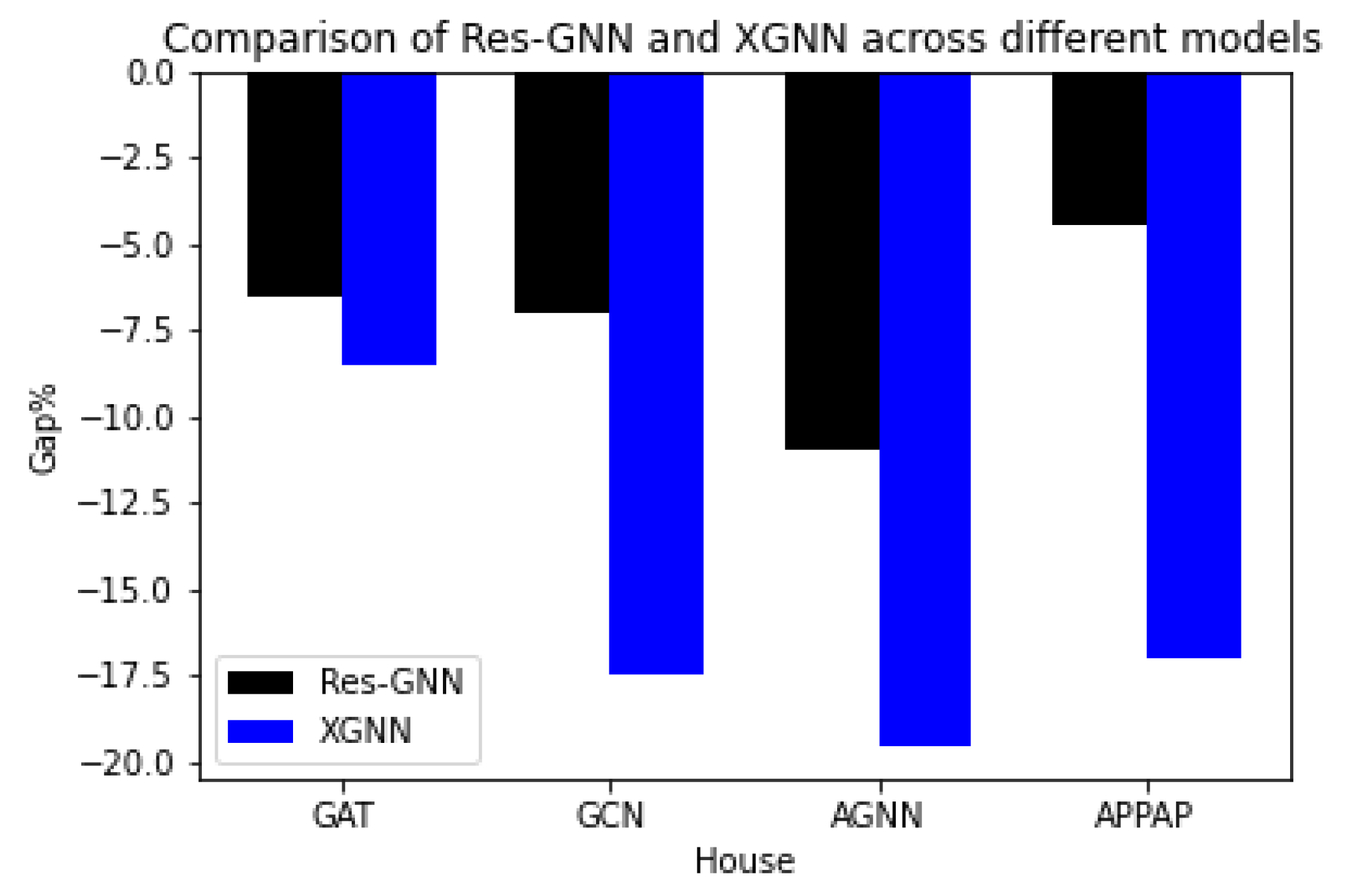
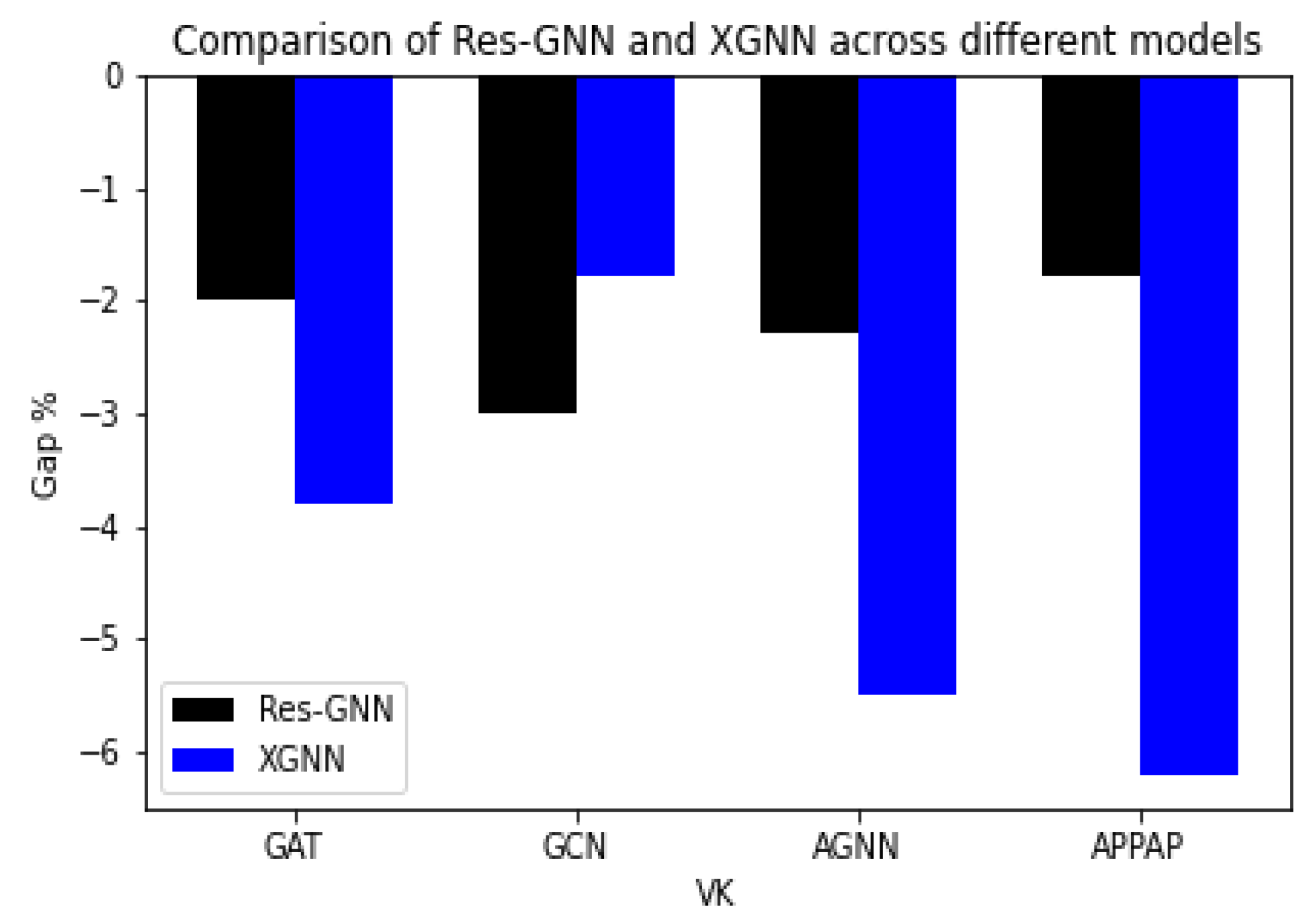
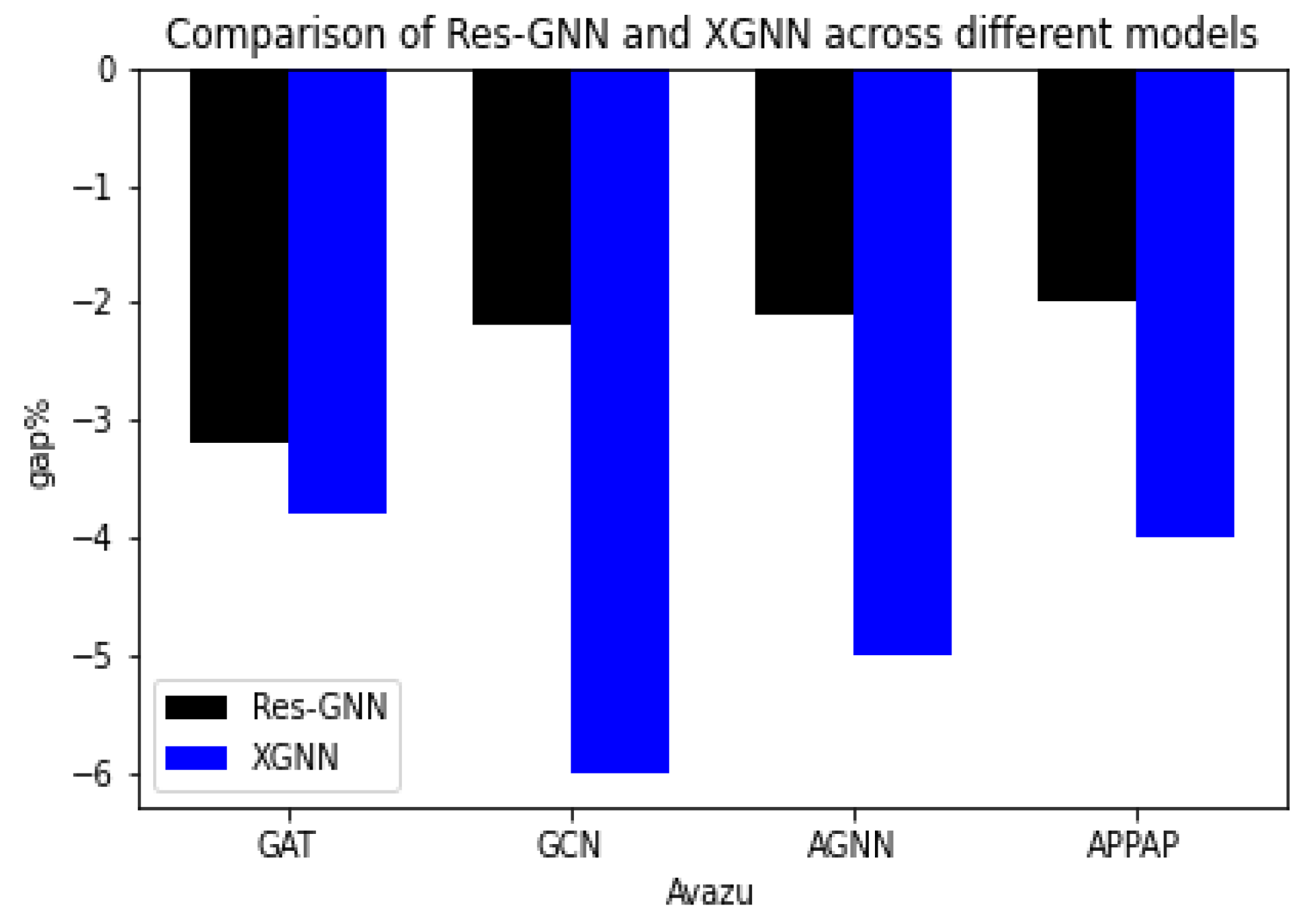
Res-GNN: First, train a GBDT model on the training set of nodes, append or replace the original node features with their predictions for all nodes, and then train a GNN on the updated features.

(11)

XGNN: Simultaneous training of XGBoost and GNN in an end-to-end manner.

4.3. Settings

For all models, we performed a hyperparametric search for a learning rate in the range of 0.1 to 0.01 and evaluated it three times to take the average. We then randomly partitioned the training, validation, and test sets at 60%, 20%, and 20%, and reported the average of the five random seeds.

4.4. Results

Table 3 presents the node prediction results. A comparison of the RMSE results from various datasets using different models reveals that XGNN significantly outperforms the previous model. When compared to the BestowGNN + C&S model for different datasets, XGNN cuts errors by 1.7% for the House dataset, 5.5% for the County dataset, 7.1% for the VK dataset, and 0.8% for the Avazu dataset. Although the Res-GNN model is not as good as the XGNN model, it improves its performance when using the XGBoost model as the GNN input. The isomorphic dataset Wiki does not perform as well as GAT because XGNN is too complex for isomorphic data, which causes the model to overfit or underfit when dealing with a single type of data. Meanwhile, the end-to-end combination FCNN-GNN outperforms the pure GNN model but falls short of XGNN. Overall, the experiments comparing these baselines illustrate that XGNN has an advantage in node prediction.

Table 3. RMSE of node prediction for different datasets.

Dataset	House	County	VK	Avazu	Wiki
CatBoost	0.63 ± 0.01	1.39 ± 0.07	7.16 ± 0.20	0.1172 ± 0.02	46,359 ± 4508
LightGBM	0.63 ± 0.01	1.4 ± 0.07	7.16 ± 0.20	0.1171 ± 0.02	49,915 ± 3643
GCN	0.63 ± 0.01	1.48 ± 0.08	7.25 ± 0.19	0.1141 ± 0.02	44,936 ± 4083
GAT	0.54 ± 0.01	1.45 ± 0.06	7.22 ± 0.19	0.1134 ± 0.01	45,916 ± 4527
APPNP	0.69 ± 0.01	1.5 ± 0.11	13.23 ± 0.12	0.1127 ± 0.01	53,426 ± 4159
AGNN	0.59 ± 0.01	1.45 ± 0.08	7.26 ± 0.20	0.1134 ± 0.02	45,982 ± 3058
FCNN	0.68 ± 0.01	1.48 ± 0.07	7.29 ± 0.21	0.118 ± 0.02	51,662 ± 2983
F-GNN	0.53 ± 0.01	1.39 ± 0.06	7.22 ± 0.20	0.1114 ± 0.02	48,491 ± 7889
BestowGNN + C&S	0.467 ± 0.01	1.145 ± 0.08	6.918 ± 0.22	0.105 ± 0.01	-
RES-GNN	0.51 ± 0.01	1.33 ± 0.08	7.07 ± 0.20	0.1095 ± 0.01	46,747 ± 4639
XGNN	0.45 ± 0.01	1.09 ± 0.08	6.847 ± 0.20	0.097 ± 0.01	49,222 ± 3743

Table 4 presents the node classification results. A comparison of the accuracy of various datasets using various models reveals that XGNN significantly outperforms the previous model. The same is true for the heterogeneous datasets House_class and VK_class; the accuracy will increase, indicating that the model has advantages for node classification of heterogeneous datasets. While the GNN model has no advantage for the Slap and DBLP datasets with sparse bag-of-words features, XGNN’s accuracy is slightly lower than the gradient descent decision tree model. The XGNN model also did not perform better in the isomorphic dataset OGB-ArXiv. This shows that XGBoost has trouble obtaining good prediction and classification results when working with sparse and homogeneous features, which hurts XGNN’s performance.

Table 4. Accuracy of node classification for different datasets.

Dataset	House	County	VK	Avazu	Wiki
CatBoost	0.63 ± 0.01	1.39 ± 0.07	7.16 ± 0.20	0.1172 ± 0.02	46,359 ± 4508
LightGBM	0.63 ± 0.01	1.4 ± 0.07	7.16 ± 0.20	0.1171 ± 0.02	49,915 ± 3643
GCN	0.63 ± 0.01	1.48 ± 0.08	7.25 ± 0.19	0.1141 ± 0.02	44,936 ± 4083
GAT	0.54 ± 0.01	1.45 ± 0.06	7.22 ± 0.19	0.1134 ± 0.01	45,916 ± 4527
APPNP	0.69 ± 0.01	1.5 ± 0.11	13.23 ± 0.12	0.1127 ± 0.01	53,426 ± 4159
AGNN	0.59 ± 0.01	1.45 ± 0.08	7.26 ± 0.20	0.1134 ± 0.02	45,982 ± 3058
FCNN	0.68 ± 0.01	1.48 ± 0.07	7.29 ± 0.21	0.118 ± 0.02	51,662 ± 2983
F-GNN	0.53 ± 0.01	1.39 ± 0.06	7.22 ± 0.20	0.1114 ± 0.02	48,491 ± 7889
BestowGNN + C&S	0.467 ± 0.01	1.145 ± 0.08	6.918 ± 0.22	0.105 ± 0.01	-
RES-GNN	0.51 ± 0.01	1.33 ± 0.08	7.07 ± 0.20	0.1095 ± 0.01	46,747 ± 4639
XGNN	0.45 ± 0.01	1.09 ± 0.08	6.847 ± 0.20	0.097 ± 0.01	49,222 ± 3743

4.5. Training Time

Previous experiments demonstrated that XGNN performs very well on a variety of datasets, so it was important to demonstrate whether XGBoost models increase training time. With early stopping and learning rate adjustment, we measured clock time to train each model until convergence. Table 5 gives the training times for all models. The experimental results show that XGNN runs faster than GNN in most cases. This demonstrates that the XGNN model, when combined with the XGBoost model, does not require extra training time and is actually more efficient than the GNN. For example, for the County dataset, XGNN is more than nine times faster than GNN. The main reason for this is that XGBoost and GNN significantly improve parallel performance by utilizing the GPU’s parallel computing power to handle the segmentation process of multiple data samples at the same time. Moreover, the GPU histogram parameter algorithm using XGBoost can store the data in the graphics memory, which is much faster than storing the data in the main memory.

Table 5. Comparison of training time(s) between XGNN and benchmark models on nodal regression.

Dataset	House	County	VK	Avazu	Wiki
CatBoost	4 ± 1	2 ± 1	24 ± 4	10 ± 1	2 ± 2
LightGBM	3 ± 0	1 ± 0	5 ± 3	3 ± 2	0 ± 0
GCN	28 ± 0	18 ± 7	38 ± 0	13 ± 3	12 ± 6
GAT	35 ± 2	19 ± 6	42 ± 4	15 ± 1	9 ± 2
APPNP	68 ± 1	34 ± 10	81 ± 3	81 ± 3	24 ± 15
AGNN	38 ± 5	28 ± 3	48 ± 3	19 ± 5	14 ± 8
FCNN	68 ± 1	2 ± 1	109 ± 35	12 ± 2	2 ± 0
F-GNN	39 ± 1	21 ± 6	48 ± 2	16 ± 1	14 ± 3
BestowGNN + C&S	52 ± 1	18 ± 0	119 ± 0	15 ± 1	-
RES-GNN	36 ± 7	7 ± 3	41 ± 1	31 ± 2	7 ± 2
XGNN	19 ± 4	2 ± 0	15 ± 0	20 ± 3	4 ± 1

4.6. Ablation Study

In this paper, we are training XGBoost in conjunction with a GNN. If we combine XGBoost with different graph neural network models, will it perform better than other models? We replace the GNN with four graph neural networks in order, where $gap=(r_m-r_{gnn})/r_{gnn}$, where $r_m$ and $r_{gnn}$ are the root-mean-square errors of this model and the GNN, respectively. We see that the root-mean-square error (RSME) of most XGNN-based models goes down across all three datasets. This suggests that XGNN can continue to perform better than other models even when using different kinds of graph neural networks. We conducted comparative experiments on three datasets. Figure 2, Figure 3 and Figure 4 depict House, VK, and Avazu.

Figure 2. Under the House dataset.

Figure 3. Under the VK dataset.

Figure 4. Under the Avazu dataset.

5. Conclusions

In this paper, we propose a new text analysis structure, XGNN, which performs very well on graph structures of heterogeneous tabular data features. Limitations in dealing with composite data structures and deficiencies in feature extraction are overcome. By training XGBoost and GNN end-to-end, we leverage the advantages of XGBoost in handling heterogeneous and categorical features, as well as the advantages of GNNs in capturing complex relationships and dependencies between nodes. Numerous tests demonstrate that the XGNN model in this paper excels in both prediction and classification tasks. Switching to other graph neural network models co-trained with XGBoost also enhances its performance. The research on XGNN models not only promotes the development of graph neural network (GNN) technology but also broadens the application of machine learning algorithms such as XGBoost. This cross-domain integration and innovation provides more possibilities for future research work. Finally, although the XGNN model has some limitations when facing isomorphic and sparse data, this is what drives us to further research and improve.

We believe that the future research direction can be in-depth research on top of graph-level prediction and subgraph detection for large models.

References

1. Ulmer, D.; Meijerink, L.; Cinà, G. Trust issues: Uncertainty estimation does not enable reliable ood detection on medical tabular data. In Proceedings of the Machine Learning for Health, Durham, NC, USA, 7–8 August 2020; pp. 341–354. [Google Scholar]
2. Clements, J.M.; Xu, D.; Yousefi, N.; Efimov, D. Sequential deep learning for credit risk monitoring with tabular financial data. arXiv 2020, arXiv:2012.15330. [Google Scholar]
3. McElfresh, D.; Khandagale, S.; Valverde, J.; Prasad, C.V.; Ramakrishnan, G.; Goldblum, M.; White, C. When do neural nets outperform boosted trees on tabular data? In Proceedings of the 37th International Conference on Neural Information Processing Systems (NIPS’23), New Orleans, LA, USA, 10–16 December 2023; pp. 76336–76369. [Google Scholar]
4. Xie, Y.; Wang, Z.; Li, Y.; Ding, B.; Gürel, N.M.; Zhang, C.; Huang, M.; Lin, W.; Zhou, J. Fives: Feature interaction via edge search for large-scale tabular data. In Proceedings of the 27th ACM SIGKDD Conference on Knowledge Discovery & Data Mining, Singapore, 14–18 August 2021; pp. 3795–3805. [Google Scholar]
5. Bentéjac, C.; Csörgő, A.; Martínez-Muñoz, G. A comparative analysis of gradient boosting algorithms. Artif. Intell. Rev. 2021, 54, 1937–1967. [Google Scholar] [CrossRef]
6. Sagi, O.; Rokach, L. Approximating XGBoost with an interpretable decision tree. Inf. Sci. 2021, 572, 522–542. [Google Scholar] [CrossRef]
7. Prokhorenkova, L.; Gusev, G.; Vorobev, A.; Dorogush, A.V.; Gulin, A. CatBoost: Unbiased boosting with categorical features. In Proceedings of the 32nd International Conference on Neural Information Processing Systems (NIPS’18), Montreal, QC, Canada, 3–8 December 2018; pp. 6639–6649. [Google Scholar]
8. Ke, G.; Meng, Q.; Finley, T.; Wang, T.; Chen, W.; Ma, W.; Ye, Q.; Liu, T.-Y. Lightgbm: A highly efficient gradient boosting decision tree. In Proceedings of the 31st International Conference on Neural Information Processing Systems (NIPS’17), Long Beach, CA, USA, 4–9 December 2017; pp. 3149–3157. [Google Scholar]
9. Grinsztajn, L.; Oyallon, E.; Varoquaux, G. Why do tree-based models still outperform deep learning on typical tabular data? Adv. Neural Inf. Process. Syst. 2022, 35, 507–520. [Google Scholar]
10. Popov, S.; Morozov, S.; Babenko, A. Neural oblivious decision ensembles for deep learning on tabular data. arXiv 2019, arXiv:1909.06312. [Google Scholar]
11. Ke, G.; Zhang, J.; Xu, Z.; Bian, J.; Liu, T.-Y. TabNN: A universal neural network solution for tabular data. In Proceedings of the International Conference on Learning Representations (ICLR 2019), New Orleans, LA, USA, 6–9 May 2019. [Google Scholar]
12. Paliwal, S.S.; Vishwanath, D.; Rahul, R.; Sharma, M.; Vig, L. Tablenet: Deep learning model for end-to-end table detection and tabular data extraction from scanned document images. In Proceedings of the 2019 International Conference on Document Analysis and Recognition (ICDAR), Sydney, Australia, 20–25 September 2019; pp. 128–133. [Google Scholar]
13. Prasad, D.; Gadpal, A.; Kapadni, K.; Visave, M.; Sultanpure, K. CascadeTabNet: An approach for end to end table detection and structure recognition from image-based documents. In Proceedings of the IEEE/CVF Conference on Computer Vision and Pattern Recognition Workshops, Seattle, WA, USA, 14–19 June 2020; pp. 572–573. [Google Scholar]
14. Guo, X.; Quan, Y.; Zhao, H.; Yao, Q.; Li, Y.; Tu, W. Tabgnn: Multiplex graph neural network for tabular data prediction. arXiv 2021, arXiv:2108.09127. [Google Scholar]
15. Telyatnikov, L.; Scardapane, S. EGG-GAE: Scalable graph neural networks for tabular data imputation. In Proceedings of the International Conference on Artificial Intelligence and Statistics, Valencia, Spain, 25–27 April 2023; pp. 2661–2676. [Google Scholar]
16. Du, L.; Gao, F.; Chen, X.; Jia, R.; Wang, J.; Zhang, J.; Han, S.; Zhang, D. TabularNet: A neural network architecture for understanding semantic structures of tabular data. In Proceedings of the 27th ACM SIGKDD Conference on Knowledge Discovery & Data Mining, Singapore, 14–18 August 2021; pp. 322–331. [Google Scholar]
17. Liao, J.C.; Li, C.-T. TabGSL: Graph Structure Learning for Tabular Data Prediction. arXiv 2023, arXiv:2305.15843. [Google Scholar]
18. Kim, M.; Choi, H.-S.; Kim, J. Explicit Feature Interaction-aware Graph Neural Network. IEEE Access 2024, 12, 15438–15446. [Google Scholar] [CrossRef]
19. Goodge, A.; Hooi, B.; Ng, S.-K.; Ng, W.S. Lunar: Unifying local outlier detection methods via graph neural networks. In Proceedings of the AAAI Conference on Artificial Intelligence, Virtual, 22 February–1 March 2022; pp. 6737–6745. [Google Scholar]
20. Hettige, B.; Wang, W.; Li, Y.-F.; Le, S.; Buntine, W. MedGraph: Structural and temporal representation learning of electronic medical records. In ECAI Digital 2020—24th European Conference on Artificial Intelligence, Virtual, 29 August–8 September 2020; IOS Press: Amsterdam, The Netherlands, 2020; pp. 1810–1817. [Google Scholar]
21. Hua, J.; Sun, D.; Hu, Y.; Wang, J.; Feng, S.; Wang, Z. Heterogeneous Graph-Convolution-Network-Based Short-Text Classification. Appl. Sci. 2024, 14, 2279. [Google Scholar] [CrossRef]
22. Cui, X.; Tao, W.; Cui, X. Affective-knowledge-enhanced graph convolutional networks for aspect-based sentiment analysis with multi-head attention. Appl. Sci. 2023, 13, 4458. [Google Scholar] [CrossRef]
23. You, J.; Ma, X.; Ding, Y.; Kochenderfer, M.J.; Leskovec, J. Handling missing data with graph representation learning. Adv. Neural Inf. Process. Syst. 2020, 33, 19075–19087. [Google Scholar]
24. Seyedrezaei, M.; Tak, A.N.; Becerik-Gerber, B. Consumption and conservation behaviors among affordable housing residents in Southern California. Energy Build. 2024, 304, 113840. [Google Scholar] [CrossRef]
25. Jia, J.; Benson, A.R. Residual correlation in graph neural network regression. In Proceedings of the 26th ACM SIGKDD International Conference on Knowledge Discovery & Data Mining, Virtual Event, 23–27 August 2020; pp. 588–598. [Google Scholar]
26. Tsitsulin, A.; Mottin, D.; Karras, P.; Müller, E. Verse: Versatile graph embeddings from similarity measures. In Proceedings of the 2018 World Wide Web Conference, Lyon, France, 23–27 April 2018; pp. 539–548. [Google Scholar]
27. Rozemberczki, B.; Allen, C.; Sarkar, R. Multi-scale attributed node embedding. J. Complex Netw. 2021, 9, cnab014. [Google Scholar] [CrossRef]
28. Song, W.; Shi, C.; Xiao, Z.; Duan, Z.; Xu, Y.; Zhang, M.; Tang, J. Autoint: Automatic feature interaction learning via self-attentive neural networks. In Proceedings of the 28th ACM International Conference on Information and Knowledge Management, Beijing, China, 3–7 November 2019; pp. 1161–1170. [Google Scholar]
29. Xiao, Y.; Zhang, Z.; Yang, C.; Zhai, C. Non-local attention learning on large heterogeneous information networks. In Proceedings of the 2019 IEEE International Conference on Big Data (Big Data), Los Angeles, CA, USA, 9–12 December 2019; pp. 978–987. [Google Scholar]
30. Ren, Y.; Liu, B.; Huang, C.; Dai, P.; Bo, L.; Zhang, J. Heterogeneous deep graph infomax. arXiv 2019, arXiv:1911.08538. [Google Scholar]
31. Hu, W.; Fey, M.; Zitnik, M.; Dong, Y.; Ren, H.; Liu, B.; Catasta, M.; Leskovec, J. Open graph benchmark: Datasets for machine learning on graphs. Adv. Neural Inf. Process. Syst. 2020, 33, 22118–22133. [Google Scholar]
32. Chen, J.; Mueller, J.; Ioannidis, V.N.; Goldstein, T.; Wipf, D. A Robust Stacking Framework for Training Deep Graph Models with Multifaceted Node Features. arXiv 2022, arXiv:2206.08473. [Google Scholar]
Disclaimer/Publisher’s Note: The statements, opinions and data contained in all publications are solely those of the individual author(s) and contributor(s) and not of MDPI and/or the editor(s). MDPI and/or the editor(s) disclaim responsibility for any injury to people or property resulting from any ideas, methods, instructions or products referred to in the content.
Article Metrics
Citations
Article Access Statistics
Multiple requests from the same IP address are counted as one view.