Robust Fixed-Time Adaptive Fault-Tolerant Control for Dynamic Positioning of Ships with Thruster Faults

Abstract

The ship dynamic positioning system has long been a subject of great interest due to the intricate and unpredictable nature of the maritime environment, which affects its dependability and timeliness. This study focuses on the issue of developing a robust, efficient, and adaptable fault-tolerant control system for ship dynamic positioning systems that experience thruster malfunctions. Firstly, we build the motion model of the ship’s dynamic positioning system with three degrees of freedom, as well as the model for faults in the thruster. A second-order fast fixed-time nonsingular sliding mode surface is formulated, and a robust adaptive control technique is introduced to counteract external environmental disturbances and model errors. The objective is to ensure rapid convergence of the system within a predetermined time frame. Simultaneously, combined with the fault-tolerant control technique, it is ensured that the dynamic positioning ship can still achieve system stability when thruster faults occur. In addition, the analysis of the Lyapunov stability criterion proves that the proposed fixed-time adaptive fault-tolerant control scheme can make the system tracking error converge within a fixed time. Finally, the effectiveness of the proposed control scheme is verified by numerical simulation results.

1. Introduction

In recent years, with the increasing attention paid to the development of marine resources, more and more dynamic positioning ships have been applied in engineering fields such as deep-sea exploration, submarine pipeline construction, and offshore oil drilling [1]. Ocean engineering ships with dynamic positioning systems can maintain a fixed position on the sea surface or track a predetermined motion trajectory in a particular posture under external environmental disturbances such as wind and waves through precise control of the ship’s thrusters [2,3]. Scholars have shown growing interest in the dynamic positioning control of surface boats. Various control algorithms, including fuzzy control, neural network control, backstepping, and hybrid control, have been presented and have shown effective control outcomes [4,5,6].

Despite significant research advancements in ship dynamic positioning, both locally and internationally, the study of fault-tolerant control in ship dynamic positioning still needs to be explored. During actual operations, ships’ thrusters endure prolonged exposure to severe maritime conditions, leading to inevitable failures. The working nature of dynamic positioning ships makes it difficult to promptly repair or replace faulty thrusters with backup thrusters [7]. Therefore, to improve the system’s reliability and ensure the safety of operations, it is necessary to design an effective fault-tolerant control scheme for dynamic positioning ships to prevent position loss even in thruster faults [8].

To achieve better tracking performance, many researchers have combined sliding mode control with different control techniques, such as neural networks, adaptive control, etc., to achieve superior control performance. Aiming at the dynamic safety constraint problem of a dynamic positioning ship under model uncertainty and unknown environmental disturbance, Liu et al. [9] proposed a robust tracking control framework based on a unified barrier function and backstepping control. They designed an observer to observe the total disturbance so that the state of the dynamic positioning ship is always kept within the safety constraint. Gong et al. [10] designed a variable-gain preset performance control scheme to improve the system’s transient and steady-state responses. Using the variable-gain technology, the positioning error dynamically adjusts the control gain, and all the system signals are ultimately uniformly bounded to ensure the preset performance. Cui et al. [11] presented a robust adaptive stabilization controller based on observers for the dynamic positioning of ships with time delays. They analyzed the stability of the proposed controller using Lyapunov stability theory and verified the method’s effectiveness through simulation experiments. Considering the dynamic positioning problem of fully actuated ships with time-varying disturbances, Dong et al. [12] developed a disturbance observer to observe unknown disturbances and designed a robust adaptive backstepping controller combined with the backstepping controller. The simulation results showed that the proposed control scheme makes all system signals uniformly bounded. However, the control schemes mentioned in the above literature can only achieve asymptotic stability of the system, which cannot guarantee the convergence of the system state within a finite time. Zhang et al. [13] proposed a finite-time controller with a fast exponential reaching law for ship dynamic systems subject to environmental disturbances and actuator constraints to ensure that the positioning error converges to zero quickly. To overcome the influence of sampling period variation on the control performance of the system, Zhang et al. [14] designed a finite-time discrete sliding mode controller, which can make the tracking error signal of the closed-loop system converge to a small area near zero within a finite time. Considering the actuator failure of the ship, Zhang et al. [15] proposed an adaptive fault-tolerant control based on event-triggering. The control scheme can still guarantee the semi-global uniform boundedness of the system tracking error in the case of actuator faults. Mu et al. [16] studied the position-constrained ship dynamic positioning output feedback control of thruster system dynamics, using a fixed-time extended state observer to compensate for the total disturbance composed of unknown disturbances and unknown dynamics. In addition, a finite-time auxiliary power system was used to handle the input saturation problem of thrusters. Finally, a robust control term was introduced to address the errors generated in controller design. The verification results indicated that the designed control strategy can enable the ship to reach and maintain the required position and heading and continuously stay within the specified operating area under the condition that all signals from the closed-loop control system are consistent and ultimately bounded.

Inspired by the above studies, this article investigates the dynamic positioning control problem of ships with unknown system dynamics, thruster faults, and external ocean disturbances. Firstly, the ship dynamic positioning control model is established considering the thruster faults. A fixed-time, non-singular sliding mode surface is designed with the sliding mode variable structure control technology and the fixed-time stability theory. On this basis, a fixed-time adaptive fault-tolerant control scheme is proposed, which can make the system stable in a fixed time. The main contributions of this article are threefold:

(1)

By creating a novel integral sliding mode surface, the fixed-time integral sliding mode controller naturally eliminates the singularity issue, overcoming a significant limitation of traditional fixed-time terminal sliding mode control.

(2)

By adopting the parameter adaptive control to estimate the square of the upper bound of the total uncertainty, the designed controller is smooth with no obvious chattering phenomenon and does not require any information on the upper bound of the total uncertainty.

(3)

The practical fixed-time stability of the closed-loop system is proven. The dynamic positioning errors under the designed controller can be reduced to about zero in the minor fields within a fixed time, even when subject to model uncertainties, external disturbances, and actuator faults.

The remainder of this work is arranged as follows: Section 2 shows the problem formulation and preliminaries. Section 3 introduces the main results. Section 4 gives the findings of the numerical simulation. Finally, Section 5 draws conclusions and recommendations for future research.

2. Problem Formulation and Preliminaries

2.1. Mathematical Model

This article focuses on adaptive fault-tolerant control of ship dynamic positioning. Therefore, based on Fossen’s proposed dynamic positioning ship model [17], a simplified three-degree-of-freedom kinematic and dynamic model is established.

$$\{\begin{array}{l}\dot{\eta }=J(\psi )\nu \\ M\dot{\nu }=-D(\nu )\nu +\tau +d\end{array}$$

(1)

where $\eta ={[x,y,\psi ]}^T$ denotes the position and heading angle of the ship vessel in the earth coordinate system; $\nu ={[u,v,r]}^T$ represents the ship’s surge velocity, sway velocity, and yaw angular velocity in the body-fixed coordinate system; $d$ denotes the external disturbance; and $\tau ={[{\tau }_u,{\tau }_v,{\tau }_r]}^T$ represents the control force and torque. $J(\psi )\in R^{3\times 3}$ represents the transfer matrix from the body-fixed coordinate to the earth coordinate, with the specific form as follows:

$$J(\psi )=\left[\begin{array}{ccc}\cos (\psi )& -\sin (\psi )& 0\\ \sin (\psi )& \cos (\psi )& 0\\ 0& 0& 1\end{array}\right]$$

(2)

The following properties are satisfied:

$$\{\begin{array}{l}{J}^T(\psi )J(\psi )=I_{3\times 3},\Vert J(\psi )\Vert =1\\ \dot{J}(\psi )=J(\psi )S(r)\\ J^T(\psi )S(r)J(\psi )=J(\psi )S(r)J^T(\psi )=S(r)\end{array}$$

(3)

The nominal inertia matrix $\overline{M}\in R^{3\times 3}$ and the nominal hydrodynamic damping matrix $\overline{D}(v)\in R^{3\times 3}$ are as follows:

$$\overline{M}=\left[\begin{array}{ccc}{m}_{11}& 0& 0\\ 0& m_{22}& m_{23}\\ 0& m_{32}& m_{33}\end{array}\right]$$

(4)

$$\overline{D}(\nu )=\left[\begin{array}{ccc}{d}_{11}(\nu )& 0& 0\\ 0& d_{22}(\nu )& d_{23}(\nu )\\ 0& d_{32}(\nu )& d_{33}(\nu )\end{array}\right]$$

(5)

where $m_{11}=m-X_{\dot{u}}$, $m_{22}=m-Y_{\dot{v}}$, $m_{23}=m{x}_g-Y_{\dot{r}}$, $m_{32}=m{x}_g-N_{\dot{v}}$, $m_{33}=I_z-N_{\dot{r}}$, $c_{13}(\nu )=-m_{11}\nu -m_{23}r$, $c_{23}(\nu )=-m_{11}u$, $d_{11}(\nu )=-X_u-X_{\left|u\right|u}\left|u\right|-X_{uuu}{\left|u\right|}^2$, $d_{22}(\nu )=-Y_v-Y_{\left|v\right|v}\left|v\right|$, $d_{23}(\nu )=-Y_r-Y_{\left|v\right|r}\left|v\right|-Y_{\left|r\right|r}\left|r\right|$, $d_{32}(\nu )=-N_v-N_{\left|v\right|v}\left|v\right|-N_{\left|r\right|v}\left|r\right|$, $d_{33}(\nu )=-N_r-N_{\left|v\right|r}\left|v\right|-N_{\left|r\right|r}\left|r\right|$, and $Y_{\dot{r}}=N_{\dot{v}}$. $m$ denotes the mass of the ship, and $I_z$ represents the inertia moment of the ship.

In practical applications, it is difficult to obtain an accurate model of the ship. Therefore, based on the nominal model and model uncertainty, the following descriptions are given [18]:

$$\begin{array}{l}M=\overline{M}+\Delta M\\ D(\nu )=\overline{D}(\nu )+\Delta D(\nu )\end{array}$$

(6)

where $\overline{M}$ and $\overline{D}(\nu )$ represent the matrices of the nominal model, and $\Delta M$ and $\Delta D(\nu )$ denote the matrices of the unmodeled dynamics. Therefore, Equation (1) can be rewritten as:

$$\{\begin{array}{l}\dot{\eta }=J(\psi )\nu \\ \overline{M}\dot{\nu }=-\overline{D}(\nu )\nu +\tau +d+f\end{array}$$

(7)

where $f=-\Delta M\dot{\nu }-\Delta D(\nu )\nu$.

In addition, considering the thruster faults, the actual control force and torque can be expressed as [19]:

$$\tau =\vartheta {\tau }_c+\delta$$

(8)

where $\vartheta =diag\left\{{\vartheta }_u,{\vartheta }_v,{\vartheta }_r\right\}$ represents the efficiency matrix of thrusters, $0<{\vartheta }_j\le 1,j=u,v,r$. If ${\vartheta }_j=1$, it indicates that the thruster is working normally; if $0<{\vartheta }_j<1$, it means that the thruster has a partial fault. $\delta \in R^3$ is the bias fault. ${\tau }_c$ denotes the command control vector calculated by the controller.

Based on the above analysis, the mathematical model of the ship, considering thruster faults and input saturation constraints, can be represented as follows:

$$\{\begin{array}{l}\dot{\eta }=J(\psi )\nu \\ \overline{M}\dot{\nu }=-\overline{D}(\nu )\nu +\vartheta {\tau }_c+\Omega \end{array}$$

(9)

where $\Omega =d+f+\delta$ represents the lumped uncertainties.

2.2. Lemmas and Assumptions

Lemma 1 [20].

If there exists a positive, definite, and continuous function  $V(x)$ that satisfies

$$\dot{V}(x)=-a{V}^p(x)-b{V}^q(x)+\theta$$

(10)

where  $a>0$,  $b>0$,  $0<p<1$, and  $q>1$, then the system is practically stable with a fixed time, and the system state can converge to the following residual set:

$$\left\{\underset{x\to T}{\lim x}|V(x)\le \min \left\{a^{-\frac{1}{p}}{(\frac{\theta }{1-\theta })}^{\frac{1}{p}},b^{-\frac{1}{q}}{(\frac{\theta }{1-\theta })}^{\frac{1}{q}}\right\}\right\}$$

(11)

where  $0<\theta <1$, and the convergence time  $T$ satisfies:

$$T\le T_{upper}=\frac{1}{a\theta (1-p)}+\frac{1}{b\theta (q-1)}$$

(12)

Lemma 2 [21].

For the following second-order system,

$$\{\begin{array}{ll}\hfill {\dot{x}}_1=& x_2\hfill \\ \hfill {\dot{x}}_2=& -l_{1}si{g}^{{\alpha }_1}{x}_1-l_1^{\prime }\mathrm{sgn}{x}_1-l_1^{\prime \prime }si{g}^{{\alpha }_1^{\prime }}{x}_1\hfill \\ & -l_{2}si{g}^{{\alpha }_2}{x}_2-l_2^{\prime }\mathrm{sgn}{x}_2-l_2^{\prime \prime }si{g}^{{\alpha }_2^{\prime }}{x}_2\hfill \end{array}$$

(13)

where $l_i>0$, $l_i^{\prime }>0$, $l_i^{\prime \prime }>0$, and $i=1,2$ and ${\alpha }_i$ and ${\alpha }_i^{\prime }$ satisfy ${\alpha }_1=\frac{\alpha }{2-\alpha }$, ${\alpha }_2=\alpha$, ${\alpha }_1^{\prime }=\frac{4-3\alpha }{2-\alpha }$, ${\alpha }_2^{\prime }=\frac{4-3\alpha }{3-2\alpha }$, and $0<\alpha <1$, then the second-order system state can converge to the equilibrium point within a fixed time $T$.

Lemma 3 [22].

For $x_1\in R$, $x_2\in R$, $p>0$, $q>0$, and $r>0$, the following inequality holds:

$${\left|x_1\right|}^p{\left|x_2\right|}^q\le \frac{p}{p+q}r{\left|x_1\right|}^{p+q}+\frac{q}{p+q}{r}^{-\frac{p}{q}}{\left|x_2\right|}^{p+q}$$

(14)

Lemma 4 [23].

For $x_i\in R$, $i=1,2,\dots ,n$, $0<p\le 1$, and $q>1$, the following inequalities hold:

$${\left({\displaystyle \sum _{i=1}^n\left|x_i\right|}\right)}^p\le {\displaystyle \sum _{i=1}^n{\left|x_i\right|}^p},{\left({\displaystyle \sum _{i=1}^n\left|x_i\right|}\right)}^q\le n^{1-q}{\displaystyle \sum _{i=1}^n{\left|x_i\right|}^q}$$

(15)

Assumption 1 [22].

The lumped uncertainty $\Omega$  is assumed to be bounded with $\Vert \Omega \Vert \le B$, where $B>0$  is an unknown constant.

3. Main Results

3.1. Controller Design

To facilitate the subsequent controller, the following coordinate transformation is introduced [24]:

$$\begin{array}{l}\xi =J(\psi )\nu \\ {\xi }_d=J({\psi }_d){\nu }_d\end{array}$$

(16)

Therefore, Equation (7) can be rewritten as:

$$\{\begin{array}{ll}\hfill \dot{\eta }& =\xi \hfill \\ \hfill \dot{\xi }& =-J(\psi ){\overline{M}}^{-1}D(J^T(\psi )\xi )J^T(\psi )\xi +S(r)\xi \hfill \\ & +J(\psi ){\overline{M}}^{-1}\vartheta {\tau }_c+J(\psi ){\overline{M}}^{-1}\Omega \hfill \end{array}$$

(17)

where $S(r)=\left[\begin{array}{ccc}0& -r& 0\\ r& 0& 0\\ 0& 0& 0\end{array}\right]$.

Similarly, the desired reference trajectory is represented as follows:

$$\{\begin{array}{l}{\dot{\eta }}_d={\xi }_d\\ {\dot{\xi }}_d=S(r_d){\xi }_d+J({\psi }_d){\overline{M}}^{-1}(-D({\nu }_d){\nu }_d+{\tau }_d)\end{array}$$

(18)

where $S(r_d)=\left[\begin{array}{ccc}0& -r_d& 0\\ r_d& 0& 0\\ 0& 0& 0\end{array}\right]$.

By defining the position tracking error ${\xi }_e=\xi -{\xi }_d$ and combining (18) and (19), we can obtain:

$$\begin{array}{cc}\hfill {\dot{\eta }}_e& ={\xi }_e\hfill \\ \hfill {\dot{\xi }}_e& =J(\psi ){\overline{M}}^{-1}\vartheta {\tau }_c-J(\psi ){\overline{M}}^{-1}D(J^T(\psi )\xi )J^T(\psi )\xi \hfill \\ & +S(r)\xi +J(\psi ){\overline{M}}^{-1}\Omega -S(r_d){\xi }_d-J({\psi }_d){\overline{M}}^{-1}(-D({\nu }_d){\nu }_d+{\tau }_d)\hfill \end{array}$$

(19)

Then, the following fixed-time nonsingular sliding surface is defined as follows:

$$\{\begin{array}{cc}\hfill s& ={\xi }_e+\phi \hfill \\ \hfill \dot{\phi }& =m_{1}si{g}^{a_1}({\eta }_e)+m_{2}si{g}^{a_2}({\eta }_e)+m_{3}sign({\eta }_e)\hfill \\ & +n_{1}si{g}^{b_1}({\xi }_e)+n_{2}si{g}^{b_2}({\xi }_e)+n_{3}sign({\xi }_e)\hfill \end{array}$$

(20)

where $m_1>0$, $m_2>0$, $m_3>0$, $n_1>0$, $n_2>0$, $n_3>0$, $0<a_1<1$, $a_2=2a_1/(a_1+1)$, $b_1=2a_1+1$, and $b_2=(2a_1+1)/(a_1+1)$.

By taking the time derivative of $s$, we obtain:

$$\begin{array}{cc}\hfill \dot{s}& ={\dot{\xi }}_e+\dot{\phi }\hfill \\ & =J(\psi ){\overline{M}}^{-1}\vartheta {\tau }_c-J(\psi ){\overline{M}}^{-1}D(J^T(\psi )\xi )J^T(\psi )\xi \hfill \\ & +S(r)\xi +J(\psi ){\overline{M}}^{-1}\Omega -{\dot{\xi }}_d+\dot{\phi }\hfill \end{array}$$

(21)

Then, a fixed-time reaching law is designed as follows:

$$\dot{s}=-k_{1}si{g}^p(s)-k_{2}si{g}^q(s)-\frac{{\widehat{B}}_{s}s}{2{\sigma }^2}$$

(22)

${\widehat{B}}_s$ denotes the estimation of $B_s=B^2$, and the adaptive update law ${\widehat{B}}_s$ is designed as:

$${\dot{\widehat{B}}}_s=-{\gamma }_1{\widehat{B}}_s+{\gamma }_2\frac{{\Vert s\Vert }^2}{2{\sigma }^2}$$

(23)

where ${\gamma }_1>0$ and ${\gamma }_2>0$.

In light of (22) and (23), the fixed-time adaptive sliding mode fault-tolerant controller is designed as:

$$\begin{array}{cc}\hfill {\tau }_c& ={\vartheta }^{-1}(\overline{M}{J}^{-1}(\psi )(-k_{1}si{g}^p(s)-k_{2}si{g}^q(s)-\frac{{\widehat{B}}_{s}s}{2{\sigma }^2}-\dot{\phi }-S(r)\xi \hfill \\ & -J(\psi ){\overline{M}}^{-1}\Omega )+\overline{D}(\nu )\nu +\overline{M}{J}^{-1}(\psi ){\dot{\xi }}_d)\hfill \end{array}$$

(24)

where $k_1>0$, $k_2>0$, $0<p<1$, $q>1$, and $\sigma >0$.

3.2. Stability Analysis

Based on the above discussions, the following Theorem 1 can be derived:

Theorem 1.

For the dynamic positioning ship fault-tolerant system (10), satisfying Assumption 1, the sliding mode surface is given by (21). Combined with the fixed-time adaptive fault-tolerant controller (25) and the adaptive law (24), all signals of the closed-loop system can be guaranteed to be stable within a fixed time in the case of thruster faults, external ocean disturbances, and model uncertainties.

Proof. 

The proof of Theorem 1 is completed in two steps. Firstly, it is proved that the tracking error can converge to the sliding mode surface within a fixed time, and then it is proved that the system can converge to the equilibrium point within a fixed time when it reaches the sliding mode surface. □

• Step 1: Consider the following Lyapunov candidate function:

  $$V=\frac{1}{2}{s}^{T}s+\frac{1}{2{\gamma }_2}{\tilde{B}}_s^2$$

  (25)

  where ${\tilde{B}}_s=B_s-{\widehat{B}}_s$ represents the estimation error.

Combining (20) and (22), taking the derivative of (26) yields:

$$\dot{V}=s^T(S(r)\xi +J(\psi ){\overline{M}}^{-1}(-\overline{D}(\nu )\nu +\vartheta {\tau }_c+\Omega )-{\dot{\xi }}_d+\dot{\phi })-\frac{1}{{\gamma }_2}{\tilde{B}}_s{\dot{\widehat{B}}}_s$$

(26)

Furthermore, substituting the fixed-time fault-tolerant controller (25) and adaptive law (24) into (27) yields:

$$\begin{array}{l}\dot{V}=s^T(-k_{1}si{g}^p(s)-k_{2}si{g}^q(s)-\frac{{\widehat{B}}_{s}s}{2{\sigma }^2}+\Omega )-{\tilde{B}}_s(-\frac{{\gamma }_1}{{\gamma }_2}{\widehat{B}}_s+\frac{{\Vert s\Vert }^2}{2{\sigma }^2})\\ =-k_1{\Vert s\Vert }^{p+1}-k_2{\Vert s\Vert }^{q+1}+s^T\Omega -\frac{B_s{\Vert s\Vert }^2}{2{\sigma }^2}+\frac{{\gamma }_1}{{\gamma }_2}{\tilde{B}}_s{\widehat{B}}_s\end{array}$$

(27)

According to Young‘s inequality and Assumption 1, the following is obtained:

$$s^T\Omega \le \frac{B^2{\Vert s\Vert }^2}{2{\sigma }^2}+\frac{{\sigma }^2}{2}=\frac{B_s{\Vert s\Vert }^2}{2{\sigma }^2}+\frac{{\sigma }^2}{2}$$

(28)

Moreover, it is not difficult to obtain:

$$\frac{{\gamma }_1}{{\gamma }_2}{\tilde{B}}_s{\widehat{B}}_s=\frac{{\gamma }_1}{{\gamma }_2}{\tilde{B}}_s{B}_s-\frac{{\gamma }_1}{{\gamma }_2}{\tilde{B}}_s^2\le \frac{{\gamma }_1}{2{\gamma }_2}{B}_s^2-\frac{{\gamma }_1}{2{\gamma }_2}{\tilde{B}}_s^2$$

(29)

Next, by substituting (29) and (30) into (28), we obtain:

$$\begin{array}{l}\dot{V}\le -k_1{\Vert s\Vert }^{p+1}-k_2{\Vert s\Vert }^{q+1}-\frac{{\gamma }_1}{2{\gamma }_2}{\tilde{B}}_s^2+\frac{{\gamma }_1}{2{\gamma }_2}{B}_s^2+\frac{{\sigma }^2}{2}\\ =-k_1{\Vert s\Vert }^{p+1}-k_2{\Vert s\Vert }^{q+1}-{\left(\frac{{\gamma }_1}{4{\gamma }_2}{\tilde{B}}_s^2\right)}^{\frac{p+1}{2}}-{\left(\frac{{\gamma }_1}{4{\gamma }_2}{\tilde{B}}_s^2\right)}^{\frac{q+1}{2}}+\Lambda \end{array}$$

(30)

where $\Lambda ={\left(\frac{{\gamma }_1}{4{\gamma }_2}{\tilde{B}}_s^2\right)}^{\frac{p+1}{2}}+{\left(\frac{{\gamma }_1}{4{\gamma }_2}{\tilde{B}}_s^2\right)}^{\frac{q+1}{2}}-\frac{{\gamma }_1}{2{\gamma }_2}{\tilde{B}}_s^2+\frac{{\gamma }_1}{2{\gamma }_2}{B}_s^2+\frac{{\sigma }^2}{2}$.

It is worth noting that $\Lambda$ has two cases that need to be discussed.

When $\frac{{\gamma }_1}{4{\gamma }_2}{\tilde{B}}_s^2\ge 1$, we obtain:

$${\left(\frac{{\gamma }_1}{4{\gamma }_2}{\tilde{B}}_s^2\right)}^{\frac{p+1}{2}}+{\left(\frac{{\gamma }_1}{4{\gamma }_2}{\tilde{B}}_s^2\right)}^{\frac{q+1}{2}}-\frac{{\gamma }_1}{2{\gamma }_2}{\tilde{B}}_s^2\le {\left(\frac{{\gamma }_1}{4{\gamma }_2}{\tilde{B}}_s^2\right)}^{\frac{q+1}{2}}-\frac{{\gamma }_1}{4{\gamma }_2}{\tilde{B}}_s^2$$

(31)

When $\frac{{\gamma }_1}{4{\gamma }_2}{\tilde{B}}_s^2<1$, combined with Lemma 3, we obtain:

$$\begin{array}{cc}\hfill {\left(\frac{{\gamma }_1}{4{\gamma }_2}{\tilde{B}}_s^2\right)}^{\frac{p+1}{2}}+{\left(\frac{{\gamma }_1}{4{\gamma }_2}{\tilde{B}}_s^2\right)}^{\frac{q+1}{2}}-\frac{{\gamma }_1}{2{\gamma }_2}{\tilde{B}}_s^2& \le {\left(\frac{{\gamma }_1}{4{\gamma }_2}{\tilde{B}}_s^2\right)}^{\frac{p+1}{2}}-\frac{{\gamma }_1}{4{\gamma }_2}{\tilde{B}}_s^2\hfill \\ & \le (1-\overline{p}){\overline{p}}^{\frac{\overline{p}}{1-\overline{p}}}\hfill \end{array}$$

(32)

where $\overline{p}=\frac{p+1}{2}$.

Assume that $\Phi$ satisfies $\Phi =\left\{{\tilde{B}}_s|\left|{\tilde{B}}_s\right|\le \lambda \right\}$, where $\lambda >0$. Then, according to (32) and (33), we obtain:

$${\left(\frac{{\gamma }_1}{4{\gamma }_2}{\tilde{B}}_s^2\right)}^{\frac{p+1}{2}}+{\left(\frac{{\gamma }_1}{4{\gamma }_2}{\tilde{B}}_s^2\right)}^{\frac{q+1}{2}}-\frac{{\gamma }_1}{2{\gamma }_2}{\tilde{B}}_s^2\le \mu$$

(33)

where $\mu$ is defined as:

$$\mu =\{\begin{array}{ll}(1-\overline{p}){\overline{p}}^{\frac{\overline{p}}{1-\overline{p}}},& \lambda <2\sqrt{\frac{{\gamma }_2}{{\gamma }_1}}\\ {\left(\frac{{\gamma }_1}{4{\gamma }_2}{\lambda }^2\right)}^{\frac{p+1}{2}}-\frac{{\gamma }_1}{4{\gamma }_2}{\lambda }^2,& \lambda \ge 2\sqrt{\frac{{\gamma }_2}{{\gamma }_1}}\end{array}$$

(34)

Substituting (34) into (31), combined with Lemma 4, we can obtain:

$$\dot{V}\le -\alpha V^{\frac{p+1}{2}}-\beta V^{\frac{q+1}{2}}+\varpi$$

(35)

where $\alpha =\min \left\{2^{\frac{p+1}{2}}{k}_1,{\left(\frac{{\gamma }_1}{2}\right)}^{\frac{p+1}{2}}\right\}$, $\beta =2^{\frac{1-q}{2}}\min \left\{2^{\frac{q+1}{2}}{k}_2,{\left(\frac{{\gamma }_1}{2}\right)}^{\frac{q+1}{2}}\right\}$, and $\varpi =\mu +\frac{{\gamma }_1}{2{\gamma }_2}{B}_s^2+\frac{{\sigma }^2}{2}$.

According to Lemma 1, the system tracking error can be stabilized within a fixed time $T_1$ and converge to the following residual set:

$$\Delta ({\eta }_e,{\xi }_e)\le \min \left\{{\left(\frac{\varpi }{\alpha (1-\epsilon )}\right)}^{\frac{2}{p+1}},{\left(\frac{\varpi }{\beta (1-\epsilon )}\right)}^{\frac{2}{q+1}}\right\}$$

(36)

where $0<\epsilon <1$. The upper bound of convergence time satisfies the following:

$$T_1\le \frac{2}{\alpha \epsilon (1-p)}+\frac{2}{\beta \epsilon (q-1)}$$

(37)

• Step 2: When the system state reaches the sliding mode surface, there is the following:

  $$s=0,\dot{s}=0$$

  (38)

Combining (20) and (21), the tracking error system can be written as follows:

$$\{\begin{array}{cc}\hfill {\dot{\eta }}_e=& {\xi }_e\hfill \\ \hfill {\dot{\xi }}_e=& -m_{1}si{g}^{a_1}({\eta }_e)-m_{2}si{g}^{a_2}({\eta }_e)-m_{3}sign({\eta }_e)\hfill \\ & -n_{1}si{g}^{b_1}({\xi }_e)-n_{2}si{g}^{b_2}({\xi }_e)-n_{3}sign({\xi }_e)\hfill \end{array}$$

(39)

According to Lemma 2, when the tracking error remains on the sliding mode surface, the tracking errors ${\eta }_e$ and ${\xi }_e$ can converge to the equilibrium point within a fixed time $T_2$. In summary, the designed fixed-time adaptive fault-tolerant control scheme can ensure the stability of the entire closed-loop system within a fixed time $T=T_1+T_2$.

Remark 1.

In Lemma 2, although the system tracking errors can converge to the origin along the sliding mode surface within a fixed time $T_2$, the upper bound of the convergence time during the sliding stage cannot be explicitly given. The detailed proof process of Lemma 2 can be found in reference [21].

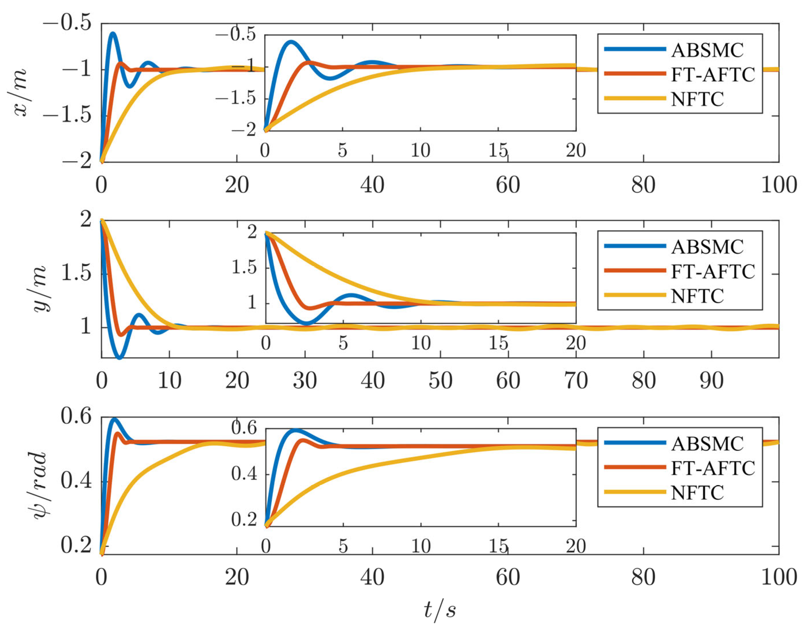
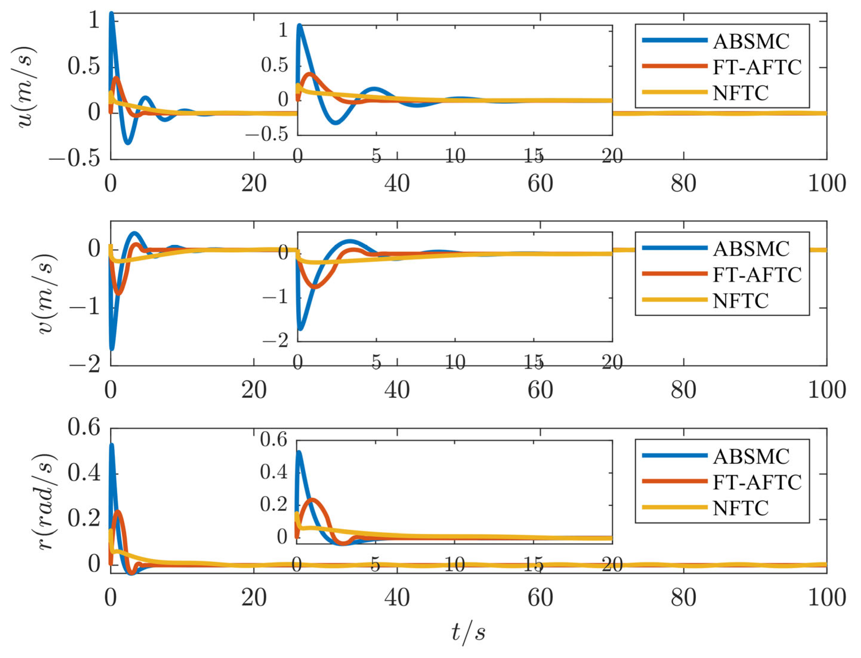
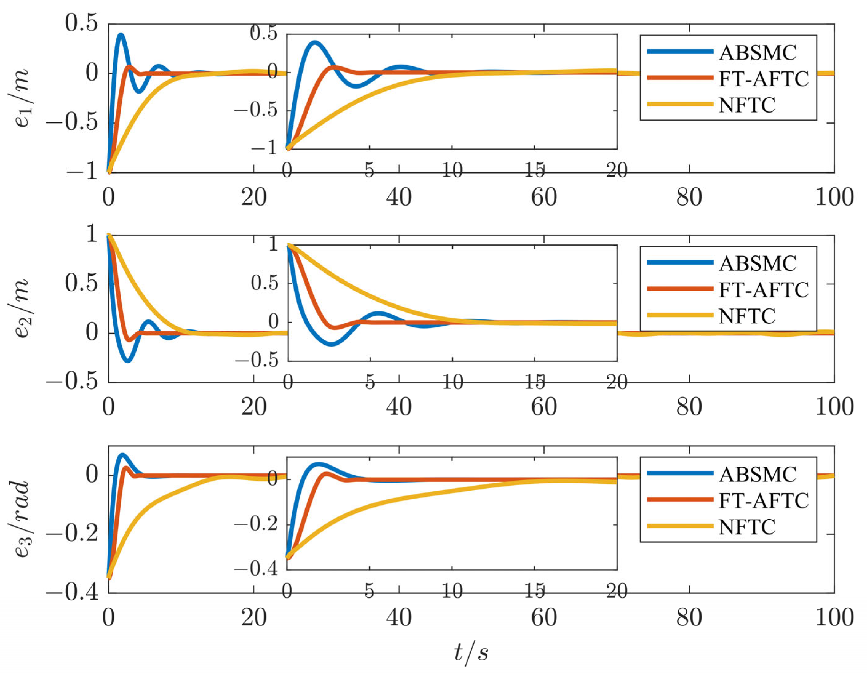
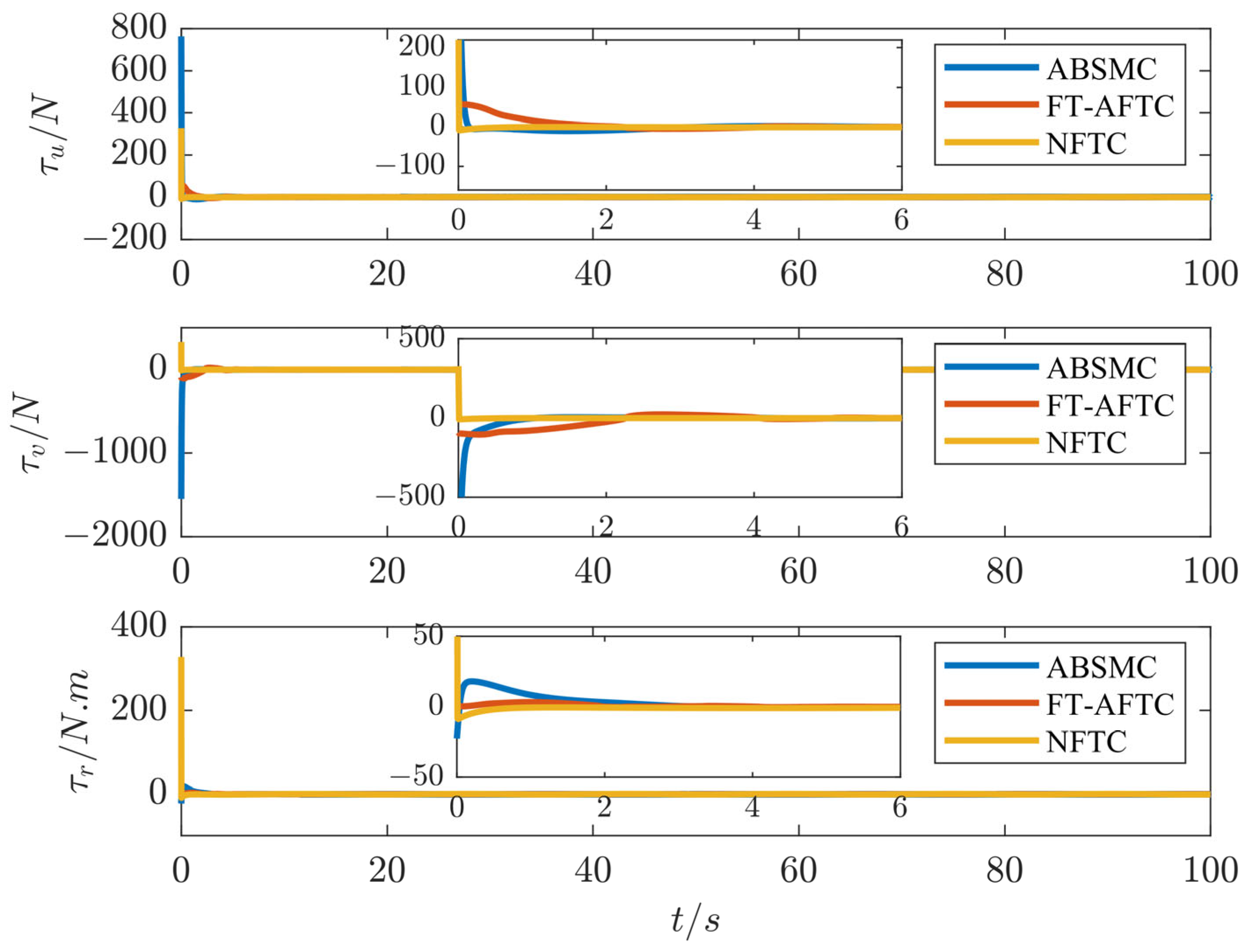
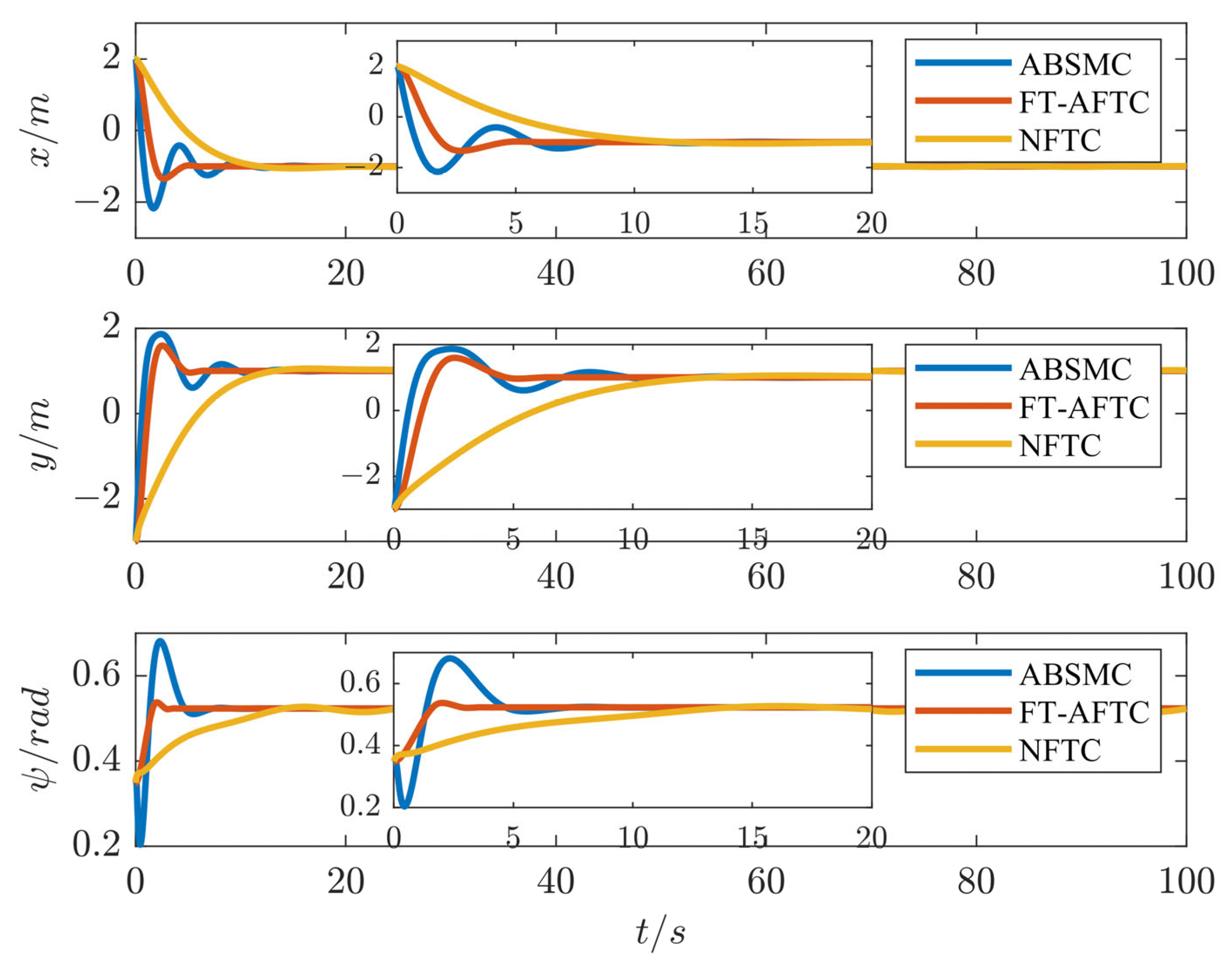
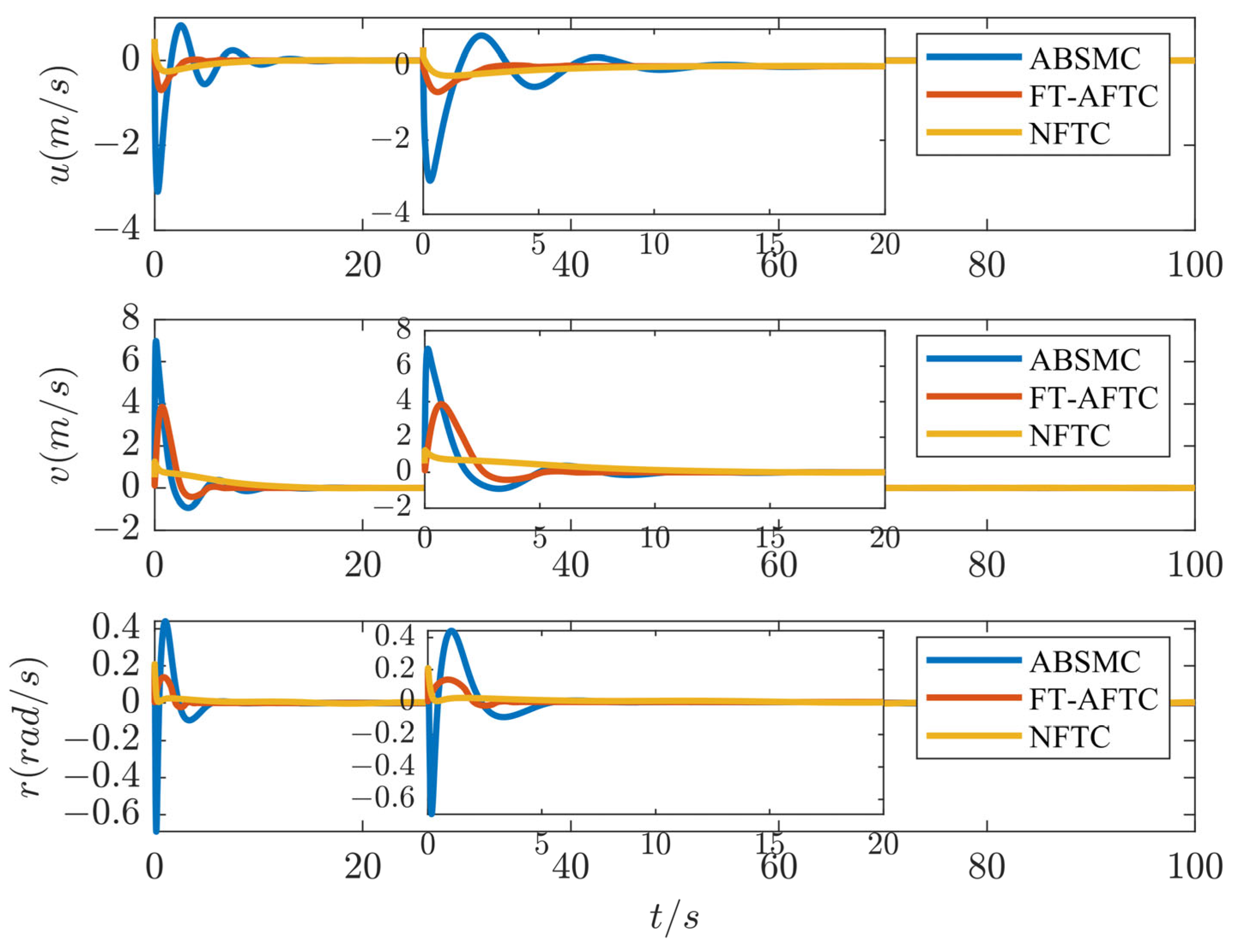
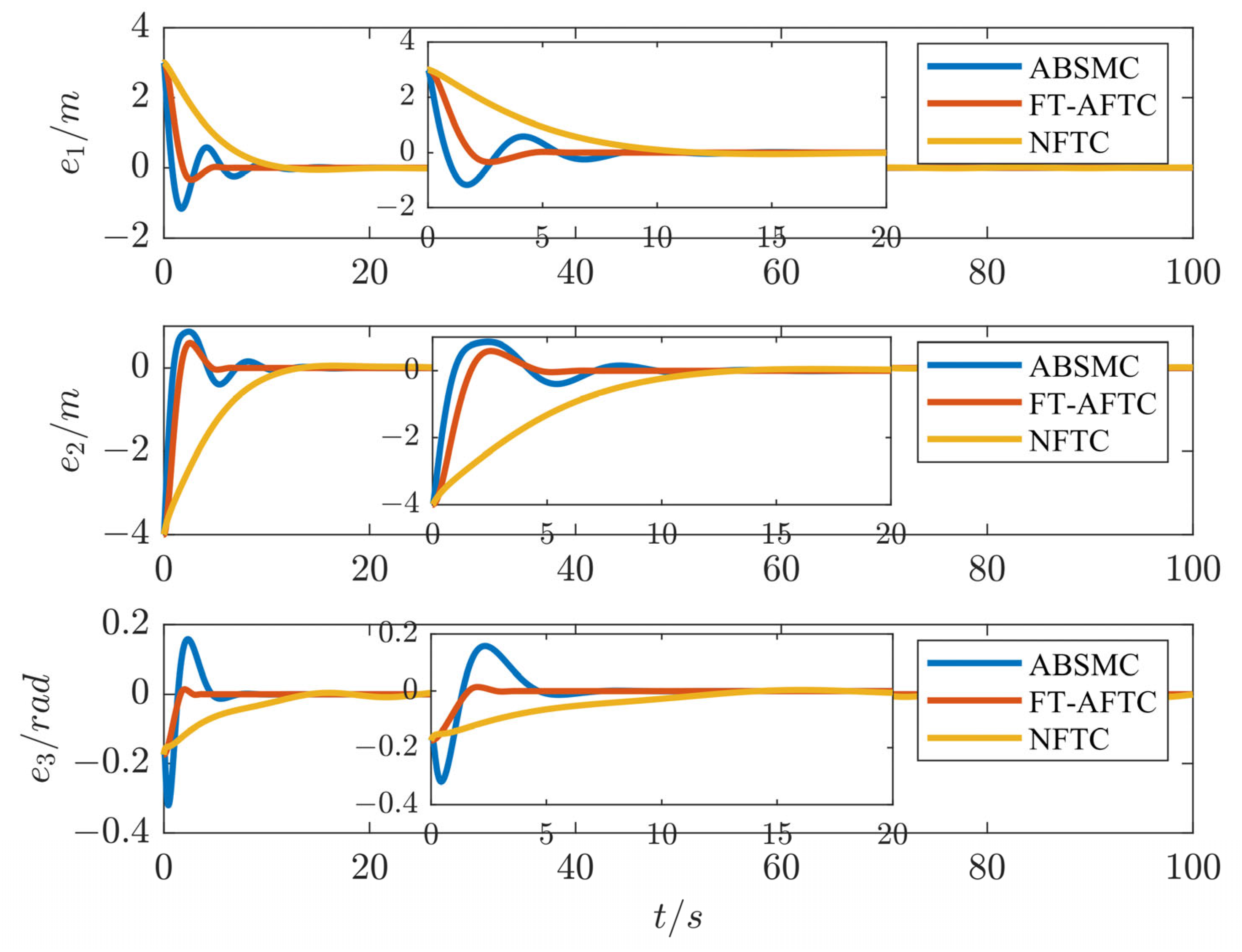
4. Simulation Results

To verify the effectiveness of the fixed-time adaptive fault-tolerant control (FT-AFTC) scheme proposed in this paper, the mathematical model of Cybership II [25] is selected to carry out simulation experiments. The detailed model parameters are listed in

Table 1. Hydrodynamic parameters of the Cybership II.

Parameters	Values	Parameters	Values	Parameters	Values
$m$	23.8	$Y_r$	0.1079	$Y_{rv}$	2
$I_z$	1.76	$N_v$	0.1052	$Y_{vr}$	1
$x_g$	0.046	$N_{vv}$	5.0437	$Y_{rr}$	3
$X_u$	−0.7225	$X_{du}$	−2	$N_{rv}$	5
$X_{uu}$	−1.3274	$Y_{dv}$	−10	$N_r$	4
$X_{uuu}$	−5.8664	$Y_{dr}$	0	$N_{vr}$	0.5
$Y_v$	-0.8612	$N_{dv}$	0	$N_{rr}$	0.8
$Y_{vv}$	−36.2823	$N_{dr}$	−1	$-$	$-$

[26]. The external time-varying disturbance is set as $d={[0.5\sin (0.2t),0.6\cos (0.4t),0.3\sin (0.5t)]}^T$. For the thruster faults model, we set $\vartheta =diag\left\{0.6+0.2\sin (0.5t),0.7+0.15\sin (0.4t),0.8+0.1\sin (0.3t)\right\}$ and $\delta ={[0.15\sin (1.5t),0.2\sin (2t),0.25\sin (0.5t)]}^T$. The controller parameters are selected as $k_1=2$, $k_2=2$, $p=\frac{7}{9}$, $q=\frac{11}{9}$, ${\gamma }_1=1$, ${\gamma }_2=1$, and $\sigma =0.01$. The initial states and the desired position are given in the following two cases: Case 1: ${\eta }_1={[-2,2,\pi /18]}^T$, ${\nu }_1={[0.1,0.1,0.1]}^T$, and ${\eta }_{d1}={[0,0,0]}^T$. Case 2: ${\eta }_2={[2,-3,\pi /9]}^T$, ${\nu }_2={[0.5,0.5,0.2]}^T$, and ${\eta }_{d2}={[-1,1,\pi /6]}^T$. Under the same conditions, the adaptive backstepping sliding mode control (ABSMC) strategy in the literature [27] and the nonlinear fault-tolerant controller (NFTC) in [28] are used for simulation comparison.

The simulation results in Case 1 are shown in Figure 1, Figure 2, Figure 3 and Figure 4. Figure 1 shows the tracking trajectory curve under the three control strategies. The FT-AFTC control scheme proposed in this paper can quickly converge to the desired position in a fixed time, even in the case of actuator failure. However, the ABSMC control strategy in reference [27] significantly overshoots the tracking trajectory and has a significantly slower convergence time than the FT-AFTC method. In addition, the convergence speed of the system under the NFTC control scheme in [28] is significantly slower than that of the FT-AFTC control method. Figure 2 shows the velocity response curves under the three controllers. Figure 3 provides the tracking error response curves under the action of the FT-AFTC control scheme, the ABSMC approach in [27], and the NFTC strategy in [28]. Compared with the ABSMC control strategy and the NFTC control scheme, the FT-AFTC algorithm can quickly converge the tracking error to the equilibrium point within a fixed time and have a minor overshoot. Additionally, the control input response curves are displayed in Figure 4. According to Figure 4, the controller proposed in this paper has less control over energy consumption. Similarly, Figure 5, Figure 6, Figure 7 and Figure 8 display the simulation results under the three control schemes in Case 2. Figure 5 and Figure 6, respectively, show the trajectory and velocity response curves of the dynamic positioning ship under the control schemes of FT-AFTC, NFTC, and ABSMC. Figure 7 displays the convergence curves of tracking errors under three different controllers. Compared with the ABSMC and NFTC approaches, the proposed FT-AFTC control scheme has faster convergence speed and better transient performance. Figure 8 shows the control input curves of three control methods. While ensuring high-precision control performance, the FT-AFTC control scheme significantly reduces control energy consumption compared to the ABSMC and NFTC schemes.

In addition, to further quantitatively evaluate the performance of the proposed algorithm, the following two performance indicators, integrated absolute error (IAE) and integrated time absolute error (ITAE), are introduced:

$$IA{E}_i={\displaystyle {\int }_0^t\left|e_i(t)\right|}dt$$

(40)

$$ITA{E}_i={\displaystyle {\int }_0^{t}t\left|e_i(t)\right|}dt$$

(41)

IAE and ITAE can reflect the control scheme’s transient and steady-state tracking accuracy. According to

Table 2. IAE of the three controllers in Case 1.

	$\mathit{I}\mathit{A}{\mathit{E}}_{\mathit{x}}$	$\mathit{I}\mathit{A}{\mathit{E}}_{\mathit{y}}$	$\mathit{I}\mathit{A}{\mathit{E}}_{\mathit{\psi }}$	$\mathit{I}\mathit{A}{\mathit{E}}_{\mathit{u}}$	$\mathit{I}\mathit{A}{\mathit{E}}_{\mathit{v}}$	$\mathit{I}\mathit{A}{\mathit{E}}_{\mathit{r}}$
FT-AFTC	1.251	1.140	0.386	0.619	1.493	0.407
ABSMC	1.470	1.381	0.482	1.792	2.502	0.501
NFTC	4.518	4.757	2.030	0.883	1.664	0.545

,

Table 3. ITAE of the three controllers in Case 1.

	$\mathit{I}\mathit{T}\mathit{A}{\mathit{E}}_{\mathit{x}}$	$\mathit{I}\mathit{T}\mathit{A}{\mathit{E}}_{\mathit{y}}$	$\mathit{I}\mathit{T}\mathit{A}{\mathit{E}}_{\mathit{\psi }}$	$\mathit{I}\mathit{T}\mathit{A}{\mathit{E}}_{\mathit{u}}$	$\mathit{I}\mathit{T}\mathit{A}{\mathit{E}}_{\mathit{v}}$	$\mathit{I}\mathit{T}\mathit{A}{\mathit{E}}_{\mathit{r}}$
FT-AFTC	1.087	1.099	0.289	0.750	2.190	1.173
ABSMC	4.298	4.189	0.437	5.128	5.711	5.790
NFTC	50.11	50.29	31.09	18.55	27.21	13.39

,

Table 4. IAE of the three controllers in Case 2.

	$\mathit{I}\mathit{A}{\mathit{E}}_{\mathit{x}}$	$\mathit{I}\mathit{A}{\mathit{E}}_{\mathit{y}}$	$\mathit{I}\mathit{A}{\mathit{E}}_{\mathit{\psi }}$	$\mathit{I}\mathit{A}{\mathit{E}}_{\mathit{u}}$	$\mathit{I}\mathit{A}{\mathit{E}}_{\mathit{v}}$	$\mathit{I}\mathit{A}{\mathit{E}}_{\mathit{r}}$
FT-AFTC	3.445	4.501	0.596	1.101	6.387	0.208
ABSMC	4.500	4.826	1.667	5.315	8.756	0.831
NFTC	12.695	17.041	12.324	1.459	5.349	0.382

and

Table 5. ITAE of the three controllers in Case 2.

	$\mathit{I}\mathit{T}\mathit{A}{\mathit{E}}_{\mathit{x}}$	$\mathit{I}\mathit{T}\mathit{A}{\mathit{E}}_{\mathit{y}}$	$\mathit{I}\mathit{T}\mathit{A}{\mathit{E}}_{\mathit{\psi }}$	$\mathit{I}\mathit{T}\mathit{A}{\mathit{E}}_{\mathit{u}}$	$\mathit{I}\mathit{T}\mathit{A}{\mathit{E}}_{\mathit{v}}$	$\mathit{I}\mathit{T}\mathit{A}{\mathit{E}}_{\mathit{r}}$
FT-AFTC	3.451	4.995	0.108	1.367	8.786	0.232
ABSMC	13.722	13.839	10.846	15.490	18.413	16.242
NFTC	77.11	96.41	27.273	20.823	42.547	12.797

, under the FT-AFTC control scheme proposed in this article, the minimum IAE and ITAE can be obtained, thus achieving the highest transient and steady-state tracking accuracy.

5. Conclusions

To solve the ship dynamic positioning control problem that involves external disturbances, model uncertainties, and thruster failures, a fixed-time adaptive fault-tolerant control technique is investigated in this study. Based on the fixed-time control theory and sliding mode control, a fixed-time sliding mode adaptive fault-tolerant controller is proposed, which can make the ship’s dynamic positioning error converge within a fixed time even if there is a thruster fault. By introducing the IAE and ITAE performance indicators, it becomes evident that the control system suggested in this article allows for faster convergence of the dynamic positioning error to the equilibrium point. Additionally, it enables an instantaneous reaction and reduces the magnitude of error overestimation. Then, a comprehensive stability analysis is performed to ensure that all the signals in the closed-loop system are fixed-time stable. Finally, simulation experiments and comparative analysis prove the effectiveness and superiority of the proposed control scheme. In further study, we will try to increase the fault-tolerant performance and robustness of multi-USV navigation by investigating fixed-time formation tracking control with actuator faults.

References

1. Zhang, G.; Yao, M.; Shan, Q.; Zhang, W. Observer-based asynchronous self-triggered control for a dynamic positioning ship with the hysteresis input. Sci. China Inf. Sci. 2022, 65, 212206. [Google Scholar] [CrossRef]
2. Mu, D.; Feng, Y.; Wang, G.; Fan, Y.; Zhao, Y. Single-parameter-learning-based robust adaptive control of dynamic positioning ships considering thruster system dynamics in the input saturation state. Nonlinear Dyn. 2022, 110, 395–412. [Google Scholar] [CrossRef]
3. Zheng, M.; Su, Y.; Yang, S.; Li, L. Reliable fuzzy dynamic positioning tracking controller for unmanned surface vehicles based on aperiodic measurement information. Int. J. Fuzzy Syst. 2023, 25, 358–368. [Google Scholar] [CrossRef]
4. Zheng, M.; Su, Y.; Yan, C. Further Stability Criteria for Sampled-Data-Based Dynamic Positioning Ships Using Takagi–Sugeno Fuzzy Models. Symmetry 2024, 16, 108. [Google Scholar] [CrossRef]
5. Shen, Y.; Zhao, Z.; Yuan, M.; Wang, S. Research on Multi-Sensor Data Fusion Positioning Method of Unmanned Ships Based on Threshold-and Hierarchical-Capacity Particle Filter. Appl. Sci. 2023, 13, 10390. [Google Scholar] [CrossRef]
6. Bae, J.H.; Kim, J.Y. Position Tracking Control of 4-DOF Underwater Robot Leg Using Deep Learning. Appl. Sci. 2024, 14, 1031. [Google Scholar] [CrossRef]
7. Liang, K.; Lin, X.; Chen, Y.; Liu, Y.; Liu, Z.; Ma, Z.; Zhang, W. Robust adaptive neural networks control for dynamic positioning of ships with unknown saturation and time-delay. Appl. Ocean Res. 2021, 110, 102609. [Google Scholar] [CrossRef]
8. Li, H.; Lin, X. Robust fault-tolerant control for dynamic positioning of ships with prescribed performance. Ocean Eng. 2024, 298, 117314. [Google Scholar] [CrossRef]
9. Liu, Y.; Lin, X.; Liang, K. Robust tracking control for dynamic positioning ships subject to dynamic safety constraints. Ocean Eng. 2022, 266, 112710. [Google Scholar] [CrossRef]
10. Gong, C.; Su, Y.; Zhang, D. Variable gain prescribed performance control for dynamic positioning of ships with positioning error constraints. J. Mar. Sci. Eng. 2022, 10, 74. [Google Scholar] [CrossRef]
11. Cui, J.; Yang, R.; Pang, C.; Zhang, Q. Observer-based adaptive robust stabilization of dynamic positioning ship with delay via Hamiltonian method. Ocean Eng. 2021, 222, 108439. [Google Scholar] [CrossRef]
12. Dong, D.; Li, J.; Yang, S.; Xiang, X. Dynamic Positioning of Ship Using Backstepping Controller with Nonlinear Disturbance Observer; NIScPR-CSIR: New Delhi, India, 2021. [Google Scholar]
13. Zhang, Y.; Liu, C.; Zhang, N.; Ye, Q.; Su, W. Finite-Time Controller Design for the Dynamic Positioning of Ships Considering Disturbances and Actuator Constraints. J. Mar. Sci. Eng. 2022, 10, 1034. [Google Scholar] [CrossRef]
14. Zhang, G.; Fu, M.; Xu, Y.; Li, J.; Zhang, W.; Fan, Z. Finite-time trajectory tracking control of dynamic positioning ship based on discrete-time sliding mode with decoupled sampling period. Ocean Eng. 2023, 284, 115030. [Google Scholar] [CrossRef]
15. Zhang, G.; Yao, M.; Zhang, W.; Zhang, W. Event-triggered distributed adaptive cooperative control for multiple dynamic positioning ships with actuator faults. Ocean Eng. 2021, 242, 110124. [Google Scholar] [CrossRef]
16. Mu, D.; Feng, Y.; Wang, G.; Fan, Y.; Zhao, Y.; Sun, X. Ship dynamic positioning output feedback control with position constraint considering thruster system dynamics. J. Mar. Sci. Eng. 2023, 11, 94. [Google Scholar] [CrossRef]
17. Fossen, T.I.; Strand, J.P. Passive nonlinear observer design for ships using Lyapunov methods: Full-scale experiments with a supply vessel. Automatica 1999, 35, 3–16. [Google Scholar] [CrossRef]
18. Wan, L.; Cao, Y.; Sun, Y.; Qin, H. Fault-tolerant trajectory tracking control for unmanned surface vehicle with actuator faults based on a fast fixed-time system. ISA Trans. 2022, 130, 79–91. [Google Scholar] [CrossRef] [PubMed]
19. Yao, Q.; Jahanshahi, H.; Golestani, M. Adaptive neural fault-tolerant control for output-constrained attitude tracking of unmanned space vehicles. Trans. Inst. Meas. Control. 2023, 45, 1229–1244. [Google Scholar] [CrossRef]
20. Gao, Z.; Guo, G. Command-filtered fixed-time trajectory tracking control of surface vehicles based on a disturbance observer. Int. J. Robust Nonlinear Control 2019, 29, 4348–4365. [Google Scholar] [CrossRef]
21. Cui, J.; Sun, H. Fixed-Time Trajectory Tracking Control of Autonomous Surface Vehicle with Model Uncertainties and Disturbances. Complexity 2020, 2020, 3281368. [Google Scholar] [CrossRef]
22. Jahanshahi, H.; Yao, Q.; Alotaibi, N.D. Fixed-time nonsingular adaptive attitude control of spacecraft subject to actuator faults. Chaos Solitons Fractals 2024, 179, 114395. [Google Scholar] [CrossRef]
23. Wang, T.; Liu, Y.; Zhang, X. Extended state observer-based fixed-time trajectory tracking control of autonomous surface vessels with uncertainties and output constraints. ISA Trans. 2022, 128, 174–183. [Google Scholar] [CrossRef] [PubMed]
24. Wang, N.; Karimi, H.R.; Li, H.; Su, S.F. Accurate trajectory tracking of disturbed surface vehicles: A finite-time control approach. IEEE/ASME Trans. Mechatron. 2019, 24, 1064–1074. [Google Scholar] [CrossRef]
25. Skjetne, R.; Fossen, T.I.; Kokotović, P.V. Adaptive maneuvering, with experiments, for a model ship in a marine control laboratory. Automatica 2005, 41, 289–298. [Google Scholar] [CrossRef]
26. Liu, H.; Weng, P.; Tian, X.; Mai, Q. Distributed adaptive fixed-time formation control for UAV-USV heterogeneous multi-agent systems. Ocean Eng. 2023, 267, 113240. [Google Scholar] [CrossRef]
27. Piao, Z.; Guo, C.; Sun, S. Adaptive backstepping sliding mode dynamic positioning system for pod driven unmanned surface vessel based on cerebellar model articulation controller. IEEE Access 2020, 8, 48314–48324. [Google Scholar] [CrossRef]
28. Qin, H.; Li, C.; Sun, Y. Adaptive neural network-based fault-tolerant trajectory-tracking control of unmanned surface vessels with input saturation and error constraints. IET Intell. Transp. Syst. 2020, 14, 356–363. [Google Scholar] [CrossRef]
Figure 1. The actual position and heading angle curves in Case 1.
Applsci 14 05738 g001
Figure 2. Curves of surge velocity, drift velocity, and yaw angular velocity in Case 1.
Applsci 14 05738 g002
Figure 3. Curves of tracking error in Case 1.
Applsci 14 05738 g003
Figure 4. Curves of thruster control input in Case 1.
Applsci 14 05738 g004
Figure 5. The actual position and heading angle curves in Case 2.
Applsci 14 05738 g005
Figure 6. Curves of surge velocity, drift velocity, and yaw angular velocity in Case 2.
Applsci 14 05738 g006
Figure 7. Curves of tracking error in Case 2.
Applsci 14 05738 g007
Figure 8. Curves of thruster control input in Case 2.
Applsci 14 05738 g008