

An Adaptive Fast Incremental Smoothing Approach to INS/GPS/VO Factor Graph Inference


Abstract
1. Introduction
- (a)
- A novel factor-graph-based INS/GPS/VO integrated navigation model is formulated, which exhibits commendable efficacy in managing dynamic alterations in sensor effectiveness, as well as accommodating asynchronous and delayed sensors;
- (b)
- The adaptive fast incremental smoothing algorithm is proposed, which demonstrates superior performance compared to the traditional incremental smoothing approach.
2. Materials and Methods
2.1. Factor Graph Model of INS/GPS/VO Integrated Navigation System
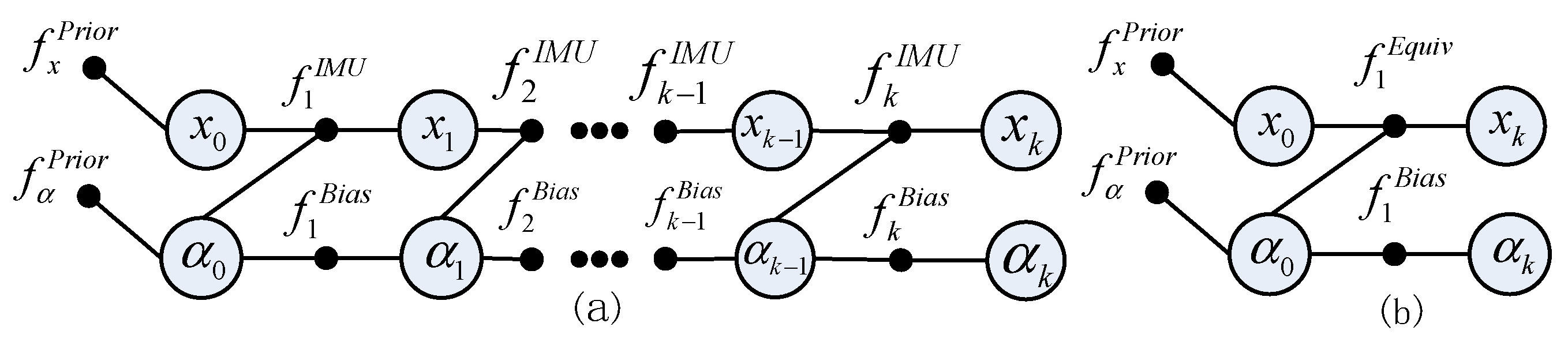
2.1.1. INS Factor Graph Model
2.1.2. Prior Factor
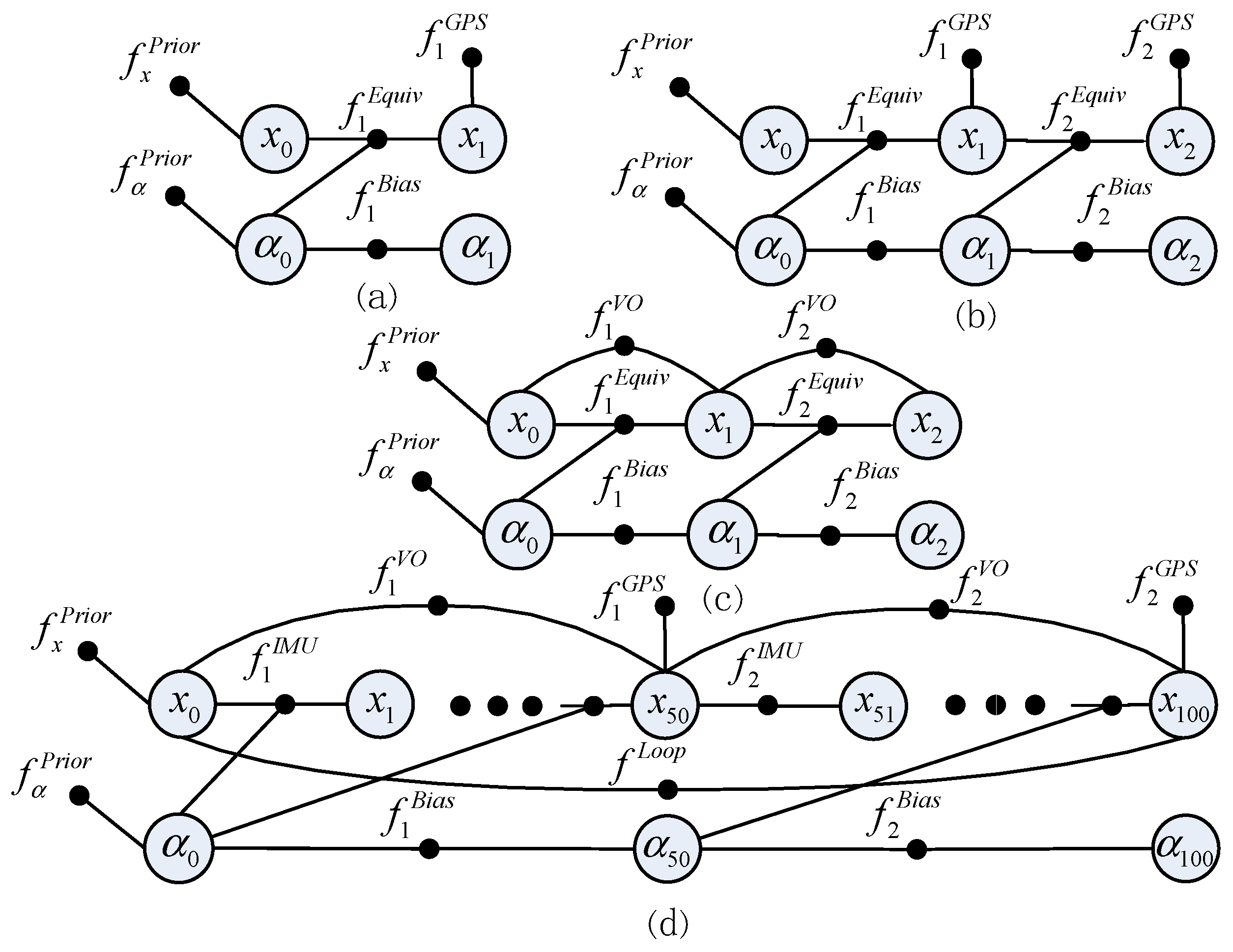
2.1.3. GPS Factor
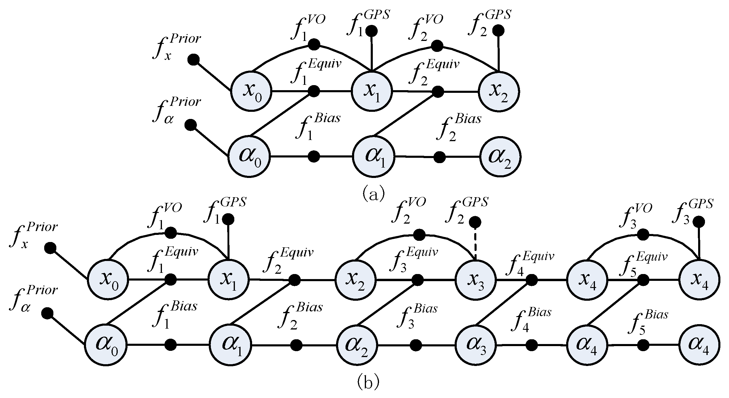
2.1.4. VO Factor
2.1.5. Loop Factor
2.2. Factor Graph Inference Algorithm for Integrated Navigation
2.2.1. Factor Graph Algorithm
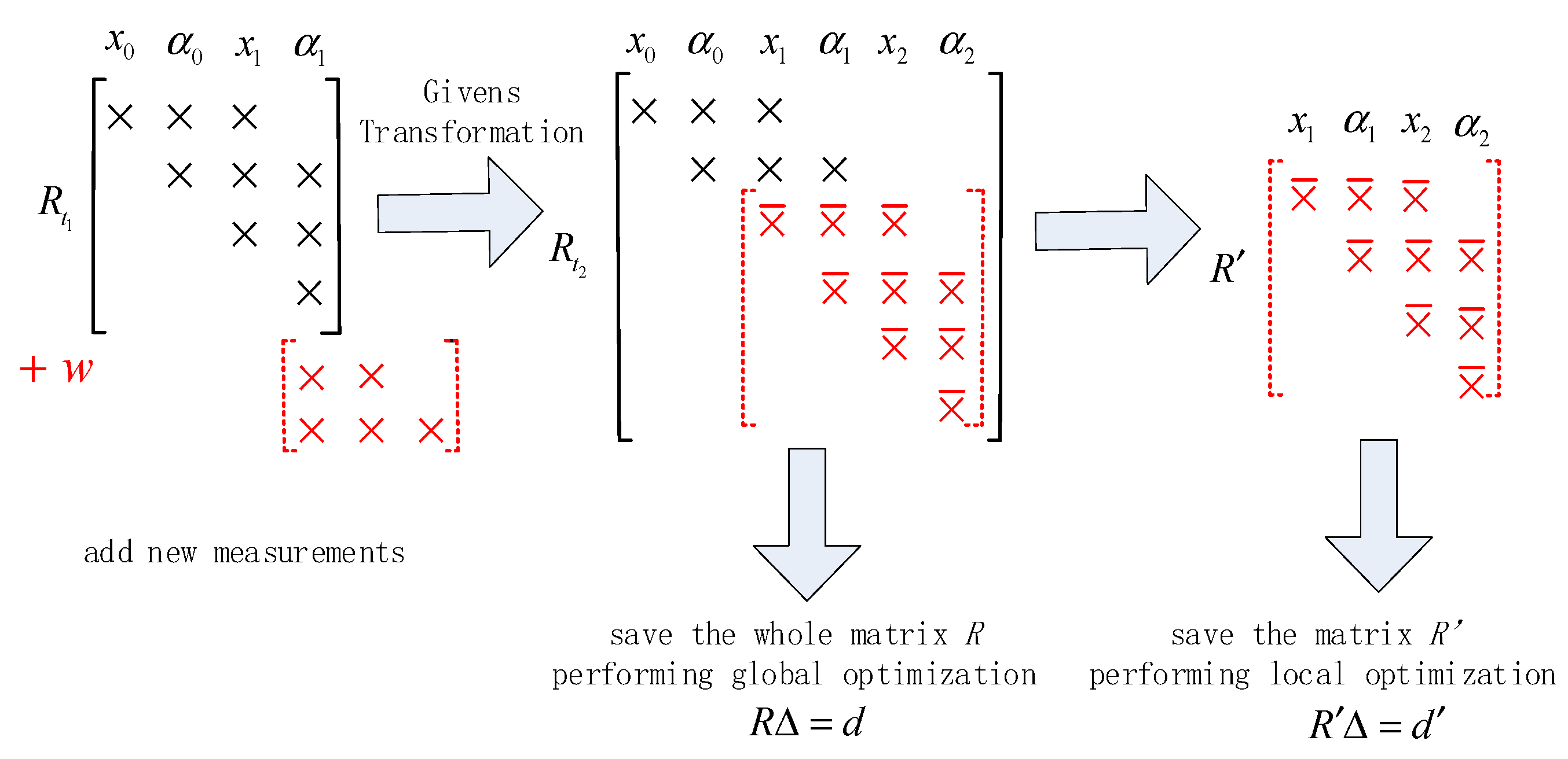
2.2.2. IS Algorithm
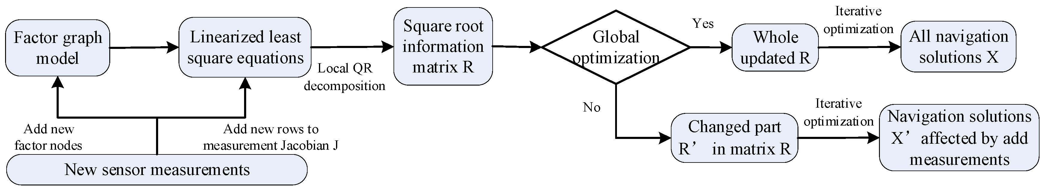
2.2.3. AFIS Algorithm
3. Results
- (1)
- Scenario 1: The simulation commences from a starting position with latitude , longitude , and altitude set at 380 m. The initial speed is 0 m/s, heading north. Following a sequence of actions, including acceleration, turning, and deceleration, the trajectory reaches a destination specified by latitude , longitude , and altitude of 380 m. The maximum speed during the trajectory is 20 m/s, and the total flight time is 250 s;
- (2)
- Scenario 2: The simulation begins at a starting position defined by latitude , longitude , and altitude of 380 m, with an initial speed of 0 m/s and heading north. Executing actions such as acceleration, turning, and deceleration, the trajectory reaches the destination defined by latitude , longitude , and altitude of 380 m, then returns to the initial position. The maximum speed during this trajectory is 20 m/s, and the total flight time is 400 s;
- (3)
- The IMU initialization data can be acquired through the application of inertial navigation’s differential equation based on the designed trajectory information. The constant drift and random drift of the gyroscope in INS is and . The constant bias and random bias of the accelerometer is 100 μg and 10 μg;
- (4)
- GPS measurement noise is characterized by a mean square error of 2 m for longitude and latitude, 5 m for height, and 0.2 m/s for speed in all three directions;
- (5)
- The initial position of VO is the same as that of the carrier, and the VO position measurement noise is quantified by a mean square error of 1 m;
- (6)
- The mean square error of the measurement noise for the Loop factor is 2 m, and the measurement equation is shown in Section 2.1.5;
- (7)
- INS sampling frequency is set at 200 Hz, the GPS update frequency at 1 Hz, and the VO output frequency at 1 Hz.
3.1. Simulation of Sensor Effectiveness with Dynamic Changes
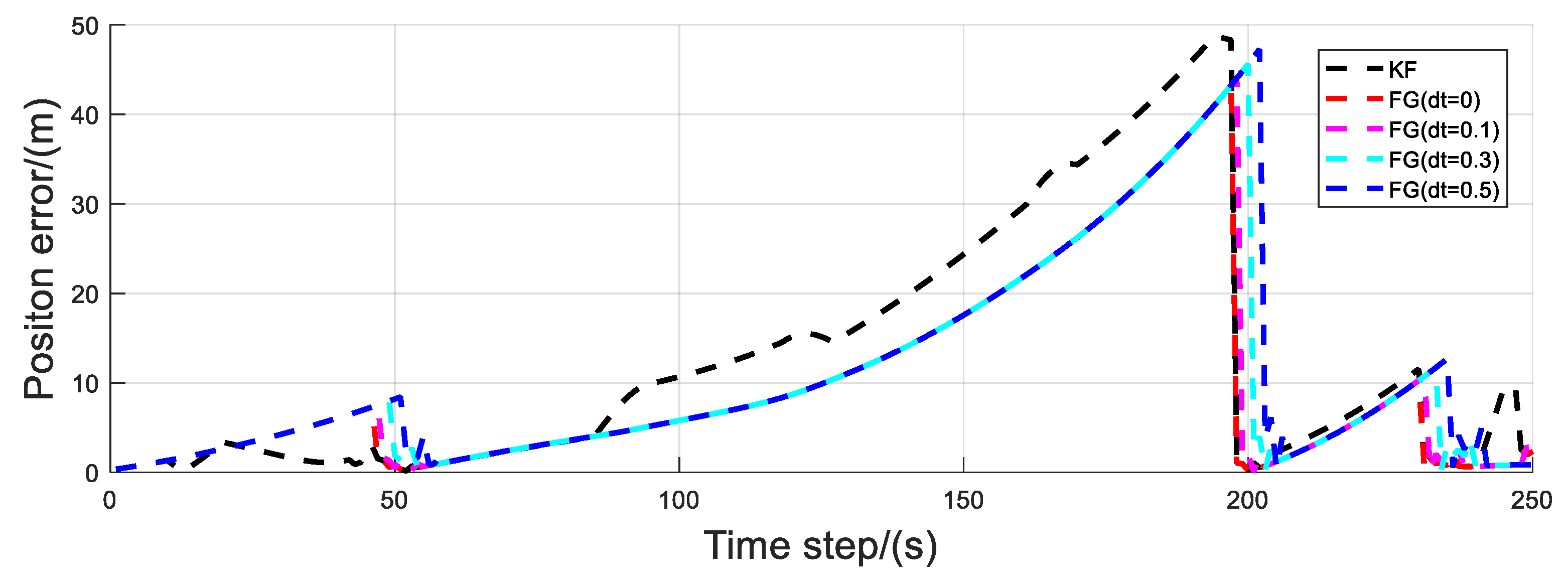
3.2. Simulation of Sensor Asynchrony and Delay
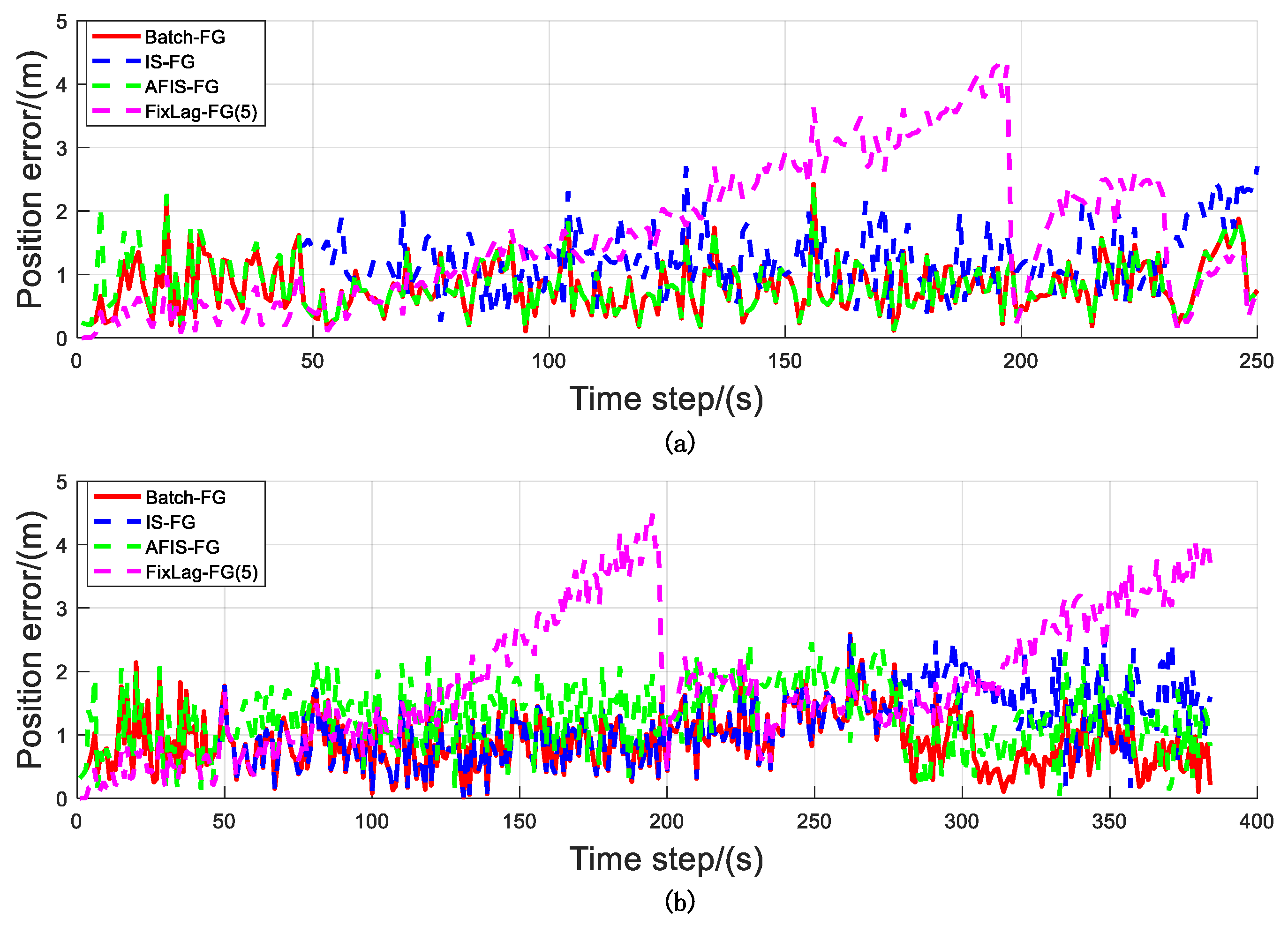
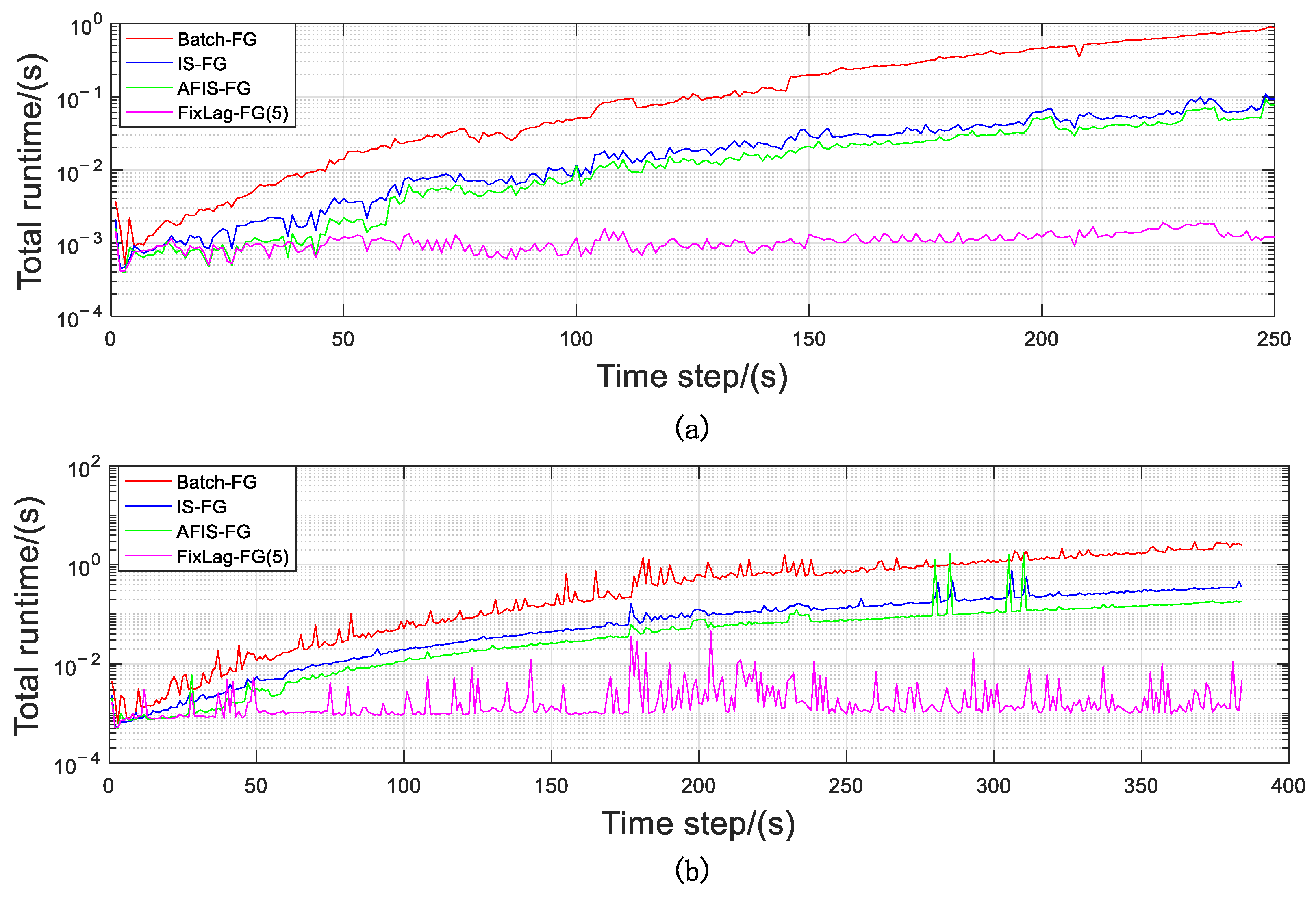
3.3. AFIS Algorithm Analysis
4. Discussion
5. Conclusions
Author Contributions
Funding
Institutional Review Board Statement
Informed Consent Statement
Data Availability Statement
Conflicts of Interest
References
- Li, W.J.; Fu, Z.Y. Unmanned aerial vehicle positioning based on multi-sensor information fusion. Geo-Spat. Inf. Sci. 2018, 21, 302–310. [Google Scholar] [CrossRef]
- Zhu, Y.; Cheng, X.; Zhou, L.; Liu, Q. Information fusion algorithm for asynchronous multi-sensors in integrated navigation systems. J. Southeast Univ. (Nat. Sci. Ed.) 2018, 48, 195–200. [Google Scholar]
- Li, S.; Li, X.; Wang, H.; Zhou, Y.; Shen, Z. Multi-GNSS PPP/INS/Vision/LiDAR tightly integrated system for precise navigation in urban environments. Inf. Fusion 2023, 90, 218–232. [Google Scholar] [CrossRef]
- Lee, Y.D.; Kim, L.W.; Lee, H.K. A tightly-coupled compressed-state constraint Kalman Filter for integrated visual-inertial-global navigation satellite system navigation in GNSS-degraded environments. IET Radar Sonar Navig. 2022, 16, 1344–1363. [Google Scholar] [CrossRef]
- Jiang, W.; Li, Y.; Rizos, C. Optimal data fusion algorithm for navigation using triple integration of PPP-GNSS, INS and terrestrial ranging system. IEEE Sens. J. 2015, 15, 5634–5644. [Google Scholar] [CrossRef]
- Li, Q.; Ben, Y.Y.; Yu, F.; Tan, J.B. Transversal strapdown INS based on reference ellipsoid for vehicle in the polar region. IEEE Trans. Veh. Technol. 2016, 65, 7791–7795. [Google Scholar] [CrossRef]
- Dryanovski, I.; Valenti, R.G.; Xiao, J.Z. An open-source navigation system for micro aerial vehicles. Auton. Robot. 2013, 34, 177–188. [Google Scholar] [CrossRef]
- Zhang, T.S.; Zhang, H.P.; Ban, Y.L.; Niu, X.J.; Liu, J.N. Tracking loop model and hardware prototype verification of GNSS/INS deep integration. In Proceedings of the 5th China Satellite Navigation Conference, Nanjing, China, 20–23 May 2014; pp. 553–572. [Google Scholar]
- Pfeifer, T.; Weissig, P.; Lange, S.; Protzel, P. Robust factor graph optimization—A comparison for sensor fusion applications. In Proceedings of the 2016 IEEE 21st International Conference on Emerging Technologies and Factory Automation, Berlin, Germany, 6–9 September 2016; pp. 1–4. [Google Scholar]
- Jiang, C.; Chen, S.; Bo, Y.; Sun, Z.; Lu, Q. Implementation and performance evaluation of a fast relocation method in a GPS/SINS/CSAC integrated navigation system hardware prototype. IEICE Electron. Express 2017, 14, 1–8. [Google Scholar] [CrossRef]
- Fu, Q.; Quan, Q.; Cai, K.Y. Robust pose estimation for multirotor UAVs using off-board monocular vision. IEEE Trans. Ind. Electron. 2017, 64, 7942–7951. [Google Scholar] [CrossRef]
- Xu, T.L.; Cui, P.Y.; Cui, H.T. Design and implementation of multi-sensor integrated navigation system of land vehicle. Syst. Eng. Electron. 2008, 30, 686–691. [Google Scholar]
- Aftatah, M.; Lahrech, A.; Abounada, A.; Soulhi, A. A GPS/INS/Odometer data for land vehicle localization in GPS denied environment. Mod. Appl. Sci. 2017, 11, 62–75. [Google Scholar] [CrossRef]
- Li, Z.K.; Wang, J.; Gao, J.X.; Yao, Y.F. The application of adaptive federated filter in GPS-INS-Odometer integrated navigation. Acta Geod. Cartogr. Sin. 2016, 45, 157–163. [Google Scholar]
- Indelman, V.; Williams, S.; Kaess, M.; Dellaert, F. Information fusion in navigation systems via factor graph based incremental smoothing. Robot. Auton. Syst. 2013, 61, 721–738. [Google Scholar] [CrossRef]
- Wu, N.; Li, B.; Wang, H.; Xing, C.W.; Kuang, J.M. Distributed cooperative localization based on Gaussian message passing on factor graph in wireless networks. Sci. China Inf. Sci. 2015, 58, 1–15. [Google Scholar] [CrossRef]
- Wen, W.; Pfeifer, T.; Bai, X.; Hsu, L. Factor graph optimization for GNSS/INS integration: A comparison with the extended Kalman filter. Navigation 2021, 68, 315–331. [Google Scholar] [CrossRef]
- Chen, M.; Xiong, Z.; Xiong, J.; Wang, R. A hybrid cooperative navigation method for UAV swarm based on factor graph and Kalman filter. Int. J. Distrib. Sens. Netw. 2022, 18, 105826. [Google Scholar] [CrossRef]
- Jiang, Y.; Ding, W.; Gao, Y. GNSS precise positioning for smartphones based on the integration of factor graph optimization and solution separation. Measurement 2022, 203, 111924. [Google Scholar] [CrossRef]
- Mourikis, A.I.; Roumeliotis, S.I. A multi-state constraint Kalman filter for visionaided inertial navigation. In Proceedings of the 2007 IEEE International Conference on Robotics and Automation, Roma, Italy, 10–14 April 2007; pp. 3565–3572. [Google Scholar]
- Mourikis, A.I.; Roumeliotis, S.I. A dual-layer estimator architecture for longterm localization. In Proceedings of the 2008 IEEE Computer Society Conference on Computer Vision and Pattern Recognition Workshops, Anchorage, AK, USA, 24–26 June 2008; pp. 1–8. [Google Scholar]
- Bryson, M.; Roberson, M.J.; Sukkarieh, S. Airborne smoothing and mapping using vision and inertial sensors. In Proceedings of the 2009 IEEE International Conference on Robotics and Automation, Kobe, Japan, 12–17 May 2009; pp. 3143–3148. [Google Scholar]
- Sibley, G.; Matthies, L.; Sukhatme, G. Sliding window filter with application to planetary landing. J. Field Robot. 2010, 27, 587–608. [Google Scholar] [CrossRef]
- Dellaert, F.; Kaess, M. Square Root SAM: Simultaneous localization and mapping via square root information smoothing. Int. J. Robot. Res. 2006, 25, 1181–1203. [Google Scholar] [CrossRef]
- Kaess, M.; Ranganathan, A.; Dellaert, F. iSAM: Incremental smoothing and mapping. IEEE Trans. Robot. 2008, 24, 1365–1378. [Google Scholar] [CrossRef]
- Williams, S.; Indelman, V.; Kaess, M.; Roberts, R.; Leonard, J.J.; Dallaert, F. Concurrent filtering and smoothing: A parallel architecture for real-time navigation and full smoothing. Int. J. Robot. Res. 2014, 33, 1544–1568. [Google Scholar] [CrossRef]
- Indelman, V.; Gurfil, P.; Rivlin, E.; Rotstein, H. Real-Time Vision-Aided Localization and Navigation Based on Three-View Geometry. IEEE Trans. Aerosp. Electron. Syst. 2012, 48, 2239–2259. [Google Scholar] [CrossRef]
- Carlone, L.; Kira, Z.; Beall, C.; Indelman, V.; Dellaert, F. Eliminating conditionally independent sets in factor graphs: A unifying perspective based on smart factors. In Proceedings of the 2014 IEEE International Conference on Robotics and Automation, Hong Kong, China, 31 May–7 June 2014; pp. 4290–4297. [Google Scholar]
- Lupton, T.; Sukkarieh, S. Visual-inertial-aided navigation for high-dynamic motion in built environments without initial conditions. IEEE Trans. Robot. 2012, 28, 61–76. [Google Scholar] [CrossRef]
- Bazeille, S.; Filliat, D. Combining odometry and visual loop-closure detection for consistent topo-metrical mapping. RAIRO—Oper. Res. 2011, 44, 365–377. [Google Scholar] [CrossRef]
- Liu, C.; Cheng, R.; Zhao, L. Loop closure detection of visual SLAM based on point and line features. J. Harbin Inst. Technol. 2020, 27, 58–64. [Google Scholar]
- An, S.; Zhu, H.; Wei, D.; Tsintotas, K.A.; Gasteratos, A. Fast and incremental loop closure detection with deep features and proximity graphs. J. Field Robot. 2022, 39, 473–493. [Google Scholar] [CrossRef]
- Kschischang, F.R.; Frey, B.J.; Loeliger, H.A. Factor graphs and the sum-product algorithm. IEEE Trans. Inf. Theory 2001, 47, 498–519. [Google Scholar] [CrossRef]
- Liu, J.W.; Cui, L.P.; Li, H.E.; Luo, X.L. Research and development on inference technique in probabilistic graphical models. Comput. Sci. 2015, 42, 1–18. [Google Scholar]
- Kaess, M.; Johannsson, H.; Roberts, R.; Ila, V.; Leonard, J.J.; Dellaert, F. ISAM2: Incremental smoothing and mapping using the Bayes tree. Int. J. Robot. Res. 2012, 31, 216–235. [Google Scholar] [CrossRef]
- Peyrard, N.; Givry, S.D.; Franc, A.; Robin, S.; Sabbadin, R.; Schiex, T.; Vignes, M. Exact and approximate inference in graphical models: Variable elimination and beyond. Comput. Sci. 2015, 35, 2454–2467. [Google Scholar]
- Meyer, G.G.L.; Pascale, M. A family of parallel QR factorization algorithms. Concurr. Pract. Exp. 2015, 8, 461–473. [Google Scholar] [CrossRef]


| Integrated Navigation Method | Wihout Delay | dt = 0.1 s | dt = 0.3 s | dt = 0.5 s | |
|---|---|---|---|---|---|
| KF | FG | FG | FG | FG | |
| Radial Error (m) | 18.32 | 14.27 | 14.57 | 15.17 | 15.81 |
| Optimization Algorithm | Batch-FG | IS-FG | AFIS-FG | FixLag-FG (5) | |
|---|---|---|---|---|---|
| Radial Error (m) | Scenario 1 | 0.907 | 1.308 | 0.940 | 1.942 |
| Scenario 2 | 1.235 | 1.570 | 1.554 | 2.588 | |
| Optimization Algorithm | Batch-FG | IS-FG | AFIS-FG | FixLag-FG (5) | |
|---|---|---|---|---|---|
| Time (s) | Scenario 1 | 54.6 | 7.4 | 4.7 | 0.2665 |
| Scenario 2 | 257.1 | 32.5 | 20.9 | 0.3971 | |
Disclaimer/Publisher’s Note: The statements, opinions and data contained in all publications are solely those of the individual author(s) and contributor(s) and not of MDPI and/or the editor(s). MDPI and/or the editor(s) disclaim responsibility for any injury to people or property resulting from any ideas, methods, instructions or products referred to in the content. |
© 2024 by the authors. Licensee MDPI, Basel, Switzerland. This article is an open access article distributed under the terms and conditions of the Creative Commons Attribution (CC BY) license (https://creativecommons.org/licenses/by/4.0/).
Share and Cite
Tian, Z.; Cheng, Y.; Yao, S. An Adaptive Fast Incremental Smoothing Approach to INS/GPS/VO Factor Graph Inference. Appl. Sci. 2024, 14, 5691. https://doi.org/10.3390/app14135691
Tian Z, Cheng Y, Yao S. An Adaptive Fast Incremental Smoothing Approach to INS/GPS/VO Factor Graph Inference. Applied Sciences. 2024; 14(13):5691. https://doi.org/10.3390/app14135691
Chicago/Turabian StyleTian, Zhaoxu, Yongmei Cheng, and Shun Yao. 2024. "An Adaptive Fast Incremental Smoothing Approach to INS/GPS/VO Factor Graph Inference" Applied Sciences 14, no. 13: 5691. https://doi.org/10.3390/app14135691
APA StyleTian, Z., Cheng, Y., & Yao, S. (2024). An Adaptive Fast Incremental Smoothing Approach to INS/GPS/VO Factor Graph Inference. Applied Sciences, 14(13), 5691. https://doi.org/10.3390/app14135691