Article

Multimodal Shot Prediction Based on Spatial-Temporal Interaction between Players in Soccer Videos

1
Graduate School of Information Science and Technology, Hokkaido University, N-14, W-9, Kita-ku, Sapporo 060-0814, Japan
2
Data-Driven Interdisciplinary Research Emergence Department, Hokkaido University, N-13, W-10, Kita-ku, Sapporo 060-0813, Japan
3
Faculty of Information Science and Technology, Hokkaido University, N-14, W-9, Kita-ku, Sapporo 060-0814, Japan
*
Author to whom correspondence should be addressed.
Appl. Sci. 2024, 14(11), 4847; https://doi.org/10.3390/app14114847
Submission received: 6 April 2024 / Revised: 24 May 2024 / Accepted: 27 May 2024 / Published: 3 June 2024
(This article belongs to the Collection Computer Science in Sport)

Abstract

:
Sports data analysis has significantly advanced and become an indispensable technology for planning strategy and enhancing competitiveness. In soccer, shot prediction has been realized on the basis of historical match situations, and its results contribute to the evaluation of plays and team tactics. However, traditional event prediction methods required tracking data acquired with expensive instrumentation and event stream data annotated by experts, and the benefits were limited to only some professional athletes. To tackle this problem, we propose a novel shot prediction method using soccer videos. Our method constructs a graph considering player relationships with audio and visual features as graph nodes. Specifically, by introducing players’ importance into the graph edge based on their field positions and team information, our method enables the utilization of knowledge that reflects the detailed match situation. Next, we extract latent features considering spatial–temporal interactions from the graph and predict event occurrences with uncertainty based on the probabilistic deep learning method. In comparison with several baseline methods and ablation studies using professional soccer match data, our method was confirmed to be effective as it demonstrated the highest average precision of 0.948, surpassing other methods.

1. Introduction

Sports analytics has become the most crucial and extensive method for tactical planning and enhancing athlete performances [1,2,3,4]. This increased importance of sports analytics can largely be attributed to significant advancements in measurement technology, which have enabled the collection of a diverse range of data [5]. In professional soccer, Electronic Performance Tracking Systems (EPTS), such as optical-based tracking systems and wearable devices, facilitate the gathering of player and ball position data, known as tracking data [6,7]. This system also monitors physical performance, including heart rate, speed, and distance covered during a match [8,9,10]. In addition to insights derived from EPTS, event stream data with details of actions such as pass, dribble, and shot are also employed. It covers who played, when, and where and is used to evaluate how each action impacted the match result more comprehensively than traditional stats [11,12]. However, acquiring such high-quality data often requires expensive measurement equipment and manual annotation by experts [13,14]. As a result, many professional teams with limited budgets and amateur athletes find it challenging to benefit from analytical techniques that rely on these data. Therefore, there is a growing demand for alternative analysis methods less reliant on costly equipment and human intervention.
Among the many evaluation methods proposed for soccer, event prediction-based performance evaluation [11,12,15,16,17,18,19] is one of the most remarkable methods in recent years. Many of these methods predict specific match events that will occur next or subsequently from tracking data and event stream data by applying machine learning techniques. In addition, it is possible to evaluate individual or series of events based on their predicted probabilities. For instance, the study in [12] performs the prediction of major attacking events (pass, dribble, cross, and shot) by using a recurrent neural network (RNN) or transformer [20]. This study also quantitatively evaluates each team’s possession with the likelihood of a shot or cross at the occurrence time of an individual event. However, event prediction methods described above use tracking data and event stream data, which require costly equipment and expert intervention. Here, the use of video data that are widely available in sports can be considered as one of the alternative approaches. With the rapid development of computer vision [21] and the release of large video datasets such as SoccerNet [22], there has been widespread research conducted on video analysis techniques (multi-player tracking [23,24,25,26], event detection/classification [27,28,29,30], video summarization [31,32], etc.) in the field of soccer analysis. A few proposals have also focused on predicting who receives the pass and the occurrence of fouls from videos and pose information of players [33,34]. Based on a wealth of visual information in match videos, the above methods provide valuable insights without using expensive instruments. Additionally, since the direct use of video reduces reliance on manual annotation, it is expected to become a more accessible and efficient solution for tactical planning and improving player performance at various competition levels. However, it is crucial to predict the occurrence of major events such as passes and shots rather than who receives a pass or the foul occurrence for player evaluation, and thus technology is required to predict these events based on soccer videos.
To tackle the aforementioned issue, we propose an event prediction method in soccer videos focusing on the shot, one of the primary events. In the proposed method, we employ unedited soccer videos, which are known as scouting videos, captured from a bird’s-eye view with a single camera. In contrast to the broadcast soccer video, the scouting video can adequately capture lengthy spatial–temporal relationships between most players since it does not focus on the ball carrier and does not include scene highlights, as shown in Figure 1. However, the extremely small image size of the ball in unedited soccer videos makes it difficult to focus on players performing actions with the ball. Hence, by constructing the relationships between players in each video frame as a graph with audio-visual information as nodes, the proposed method enables shot prediction from those videos. To introduce the importance of players based on field position and team information into the graph edge, we take advantage of knowledge that reflects detailed match situations. Then, our method extracts latent features from graphs by incorporating graph convolutional networks (GCNs) [35] and a graph convolutional recurrent network (GCRN) [36]. The graph convolutional recurrent neural network (GCRNN), which combines the above two deep learning methods, enables the extraction of latent features that consider both spatial and temporal relationships of the graph. Finally, the proposed method predicts shots with Bayesian neural networks (BNNs) [37]. The BNN is a method that can make predictions with uncertainty by introducing probability distributions for the weight parameters of the neural network. Thus, the BNN enables more reliable predictions than conventional methods based on deterministic machine learning. Note that we have previously presented the preliminary results in previous studies [38,39,40,41], where we demonstrated the effectiveness of incorporating visual information and players’ distances into graphs to achieve shot prediction from soccer videos.
In summary, the main contributions of our method are as follows:
  • For the shot prediction from soccer videos, we use a graph that introduces soccer-specific knowledge (players’ importance based on the field positions and team information) with audio-visual information as graph nodes.
  • Predicting and obtaining uncertainty with BNNs enables us to provide more robust predictions.
The remainder of the paper is organized as follows. In Section 2, we describe the shot prediction method based on multimodal features in soccer videos with GCRNN and BNNs. Experimental results and the discussion are presented in Section 3 to verify the effectiveness of the proposed method. Finally, we conclude our work in Section 4.

2. Proposed Multimodal Shot Prediction in Soccer Videos

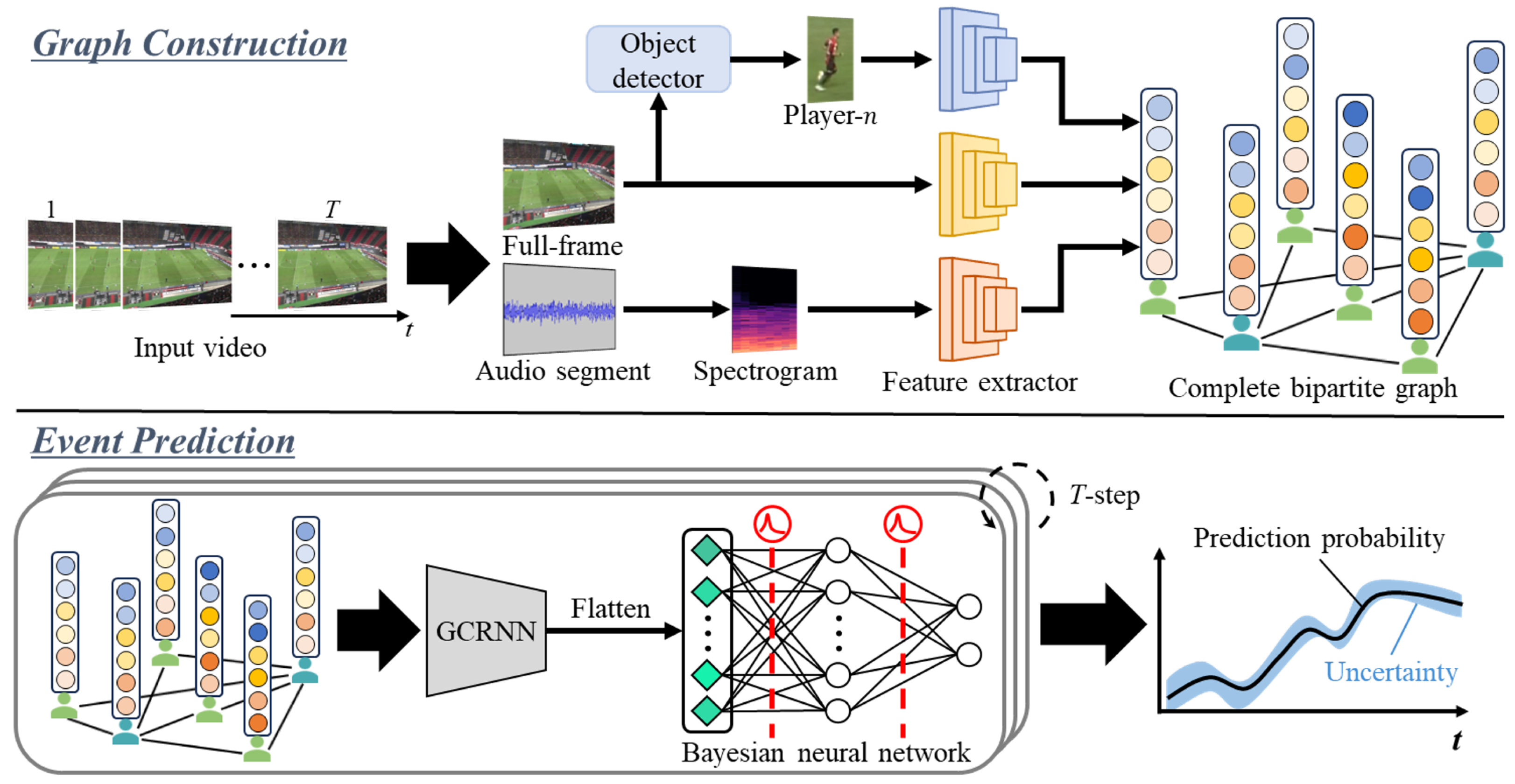
We explain the details of the proposed multimodal shot prediction method in soccer videos, as shown in Figure 2. In the proposed method, we use a graph with audio-visual features obtained from the input soccer videos as nodes. To enhance the feature representation capability, we construct a complete bipartite graph that introduces players’ importance based on their field positions and teams into the graph edge. This is described in more detail in Section 2.1. After constructing the graph, the proposed method extracts latent features through GCRNN. In this way, our method can make predictions with latent features that incorporate relationships between connected nodes and between graphs of different time steps, which correspond to spatial–temporal relationships. This is discussed further in Section 2.2. As a final step, we achieve the probability predictions of shot occurrence while accounting for uncertainty with BNNs, which is explained in Section 2.3.

2.1. Graph Construction

To effectively incorporate the match situation obtained from the soccer video, we employ the relationship between players in each frame as a graph. In the proposed method, we obtain audio segments and two types of images with full-frame size and each player region, respectively, at each time step from the soccer video. Although the audio segment does not include commentary, it contains the cheers of spectators and other auditory responses, which are considered to indicate the importance of the play and the tension involved. Especially, significant or sudden increases in cheers suggest a high likelihood of important plays, such as scoring opportunities or plays leading to them, making it effective for shot prediction. As for the object detector, we employ Mask R-CNN [42], which also performs instance segmentation simultaneously. The detected humans are used for classifying the team, referee, or other class that each detected person belongs to [43]. After converting the audio sequence into a spectrogram image, we extract features from the respective type of image. As feature extractors in the proposed method, we use ResNet-101 [44] pre-trained with ImageNet [45]. Then, to enhance the representation capability of the node features, the proposed method utilizes the features that concatenated all types of extracted audio-visual features as graph nodes X t R N × 3 D calculated through the following equation:
X t = x 1 , t player ; x t frame ; x t audio , x 2 , t player ; x t frame ; x t audio , , x N , t player ; x t frame ; x t audio ,
where x n , t player R D ( n = 1 , , N ; N representing the total number of detected players) is the visual feature of the n -th player’s region at time step t. x t frame R D and x t audio R D are audio and visual features of the full-frame image and the audio segment, respectively. Notably, D denotes the dimension of features. In this way, with the use of audio-visual information as graph nodes, the proposed method can construct a graph that has high feature representation capability.
Next, we describe the detailed settings of the graph edge in the proposed method. In soccer as a dynamic team sport, players’ positions on the pitch and their relative distances from other players dramatically change over time. All of these factors significantly contribute to the instantaneous understanding of the players’ environment and their decision-making [46,47]. Thus, we use the graph edge based on players’ field positions and the team information, as well as their distances from other players. The weights of the graph edges at time step t are represented by the adjacency matrix A t R N × N as follows:
A t ( i j ) = 0 ( team ( i ) = team ( j ) ) a t ( i j ) i j a t ( i j ) ( team ( i ) team ( j ) ) ,
a t ( i j ) = exp | | p t ( i ) p t ( j ) | | xG ( p t ( i ) ) × w a ,
where p t ( · ) denotes the 2D position on the field of each player, and w a is the edge weight coefficient. The function xG ( · ) is the expected goals (xG) at the attacking player’s position. In the proposed method, we employ the xG shown in Figure 3. It is established based on data provided by American Soccer Analysis (https://www.americansocceranalysis.com/, accessed on 4 April 2024) and is assigned a value based on the mean xG of shots in that zone in Major League Soccer matches. Furthermore, the weights are connected to players of only different teams, that is, in a complete bipartite graph. In soccer, the closer the distance between players, the more important it is to consider their relationships. Since the relationships between distant players may introduce noise, the proposed method attenuates the influence of connections between distant nodes, thereby focusing primarily on relationships between nearby nodes with the exponential function exp ( · ) . By incorporating xG, we enable predictions that focus on offensive players with a high likelihood of taking a shot and the defensive players around them. From the above, we can construct the weighted edge that considers the players’ importance and the relationship between players. By constructing such a graph, we can utilize the player interaction that closely reflects the complex match situation and affects the decision-making.

2.2. Graph Convolutional Recurrent Neural Network

To learn the spatial–temporal interaction of graphs and calculate latent features, we adopt GCRNN. In previous studies [48,49,50], several architectures of GCRNN have been proposed. The basic GCRNN architecture first updates the graph node features by applying a GCN to the graph data. The updated graph features are used to acquire hidden states by RNNs or its derivative methods such as gated recurrent unit (GRU) [51] and long short-term memory (LSTM) [52]. By inputting such hidden states to the GCN at the next time step, the node features of the graph can be updated to take into account not only the spatial relationships of the graph but also the temporal-dependent relationships. In the GCRNN model used in the proposed method, as input to the constructed graph in Section 2.1, we calculate the latent feature F t R N × D through the following equation:
F t = ReLU ( A ^ t [ ReLU ( A ^ t X t W f ( 0 ) ) ; H t 1 ] W f ( 1 ) ) ,
A ^ t = I N + D 1 2 A t D 1 2 .
Here, A ^ t represents the normalized adjacency matrix with added self-connections. I N and D are the identity and degree matrices, respectively. W f ( 0 ) R 3 D × D and W f ( 1 ) R 2 D × D are trainable weight matrices. ReLU ( · ) = max ( 0 , · ) is a widely used activation function in neural networks. The proposed method uses two stacked GCN layers to calculate latent feature F t . In the constructed complete bipartite graph, the node features are propagated two hops away in the graph, which means that the graph is updated by considering all players through the players of the opposite team. Furthermore, the final layer of GCNs is enhanced with the hidden state H t 1 R N × D of the GRU-based GCRN at the previous time step. H t 1 is calculated from the following equation:
Z t = β ( W x z G G t + W h z G H t 1 ) ,
R t = β ( W x r G G t + W h r G H t 1 ) ,
H ˜ t = tanh ( W x h G G t + W h h G ( R t H t 1 ) ) ,
H t = ( 1 Z t ) H ˜ t + Z t H t 1 .
To determine the hidden state H t at each time step, GCRN uses the update gate Z t R N × D , the reset gate R t R N × D , and the new memory content H ˜ t R N × D . The update gate Z t helps determine how much past information to retain and pass to the next time step. The reset gate R t determines how much past information to forget. The new memory content H ˜ t is composed of the input G t and the past information retained by the reset gate R t . Each gate of the GCRN receives the graph G t = ( [ X t ; F t ] , A t ) with features that combine the initial graph node and the nodes obtained through GCNs. The operator G is the graph convolution operator, and ⊙ denotes the Hadamard product. β ( · ) and tanh ( · ) are the sigmoid function and the hyperbolic tangent function, respectively. W x · R D × 4 D and W h · R D × D are trainable weight matrices for computing update gates, reset gates, and candidate hidden states at time step t. This process allows the hidden state to be obtained while considering both graph-specific and latent features. In this way, the proposed method calculates latent features while capturing the spatial–temporal interactions.

2.3. Uncertainty-Based Event Prediction

In this subsection, we describe the uncertainty-based prediction and the loss function for the optimization of the proposed model.

2.3.1. Construction with Bayesian Neural Networks

The proposed model finally predicts the shot occurrence with BNNs. The Bayesian approach estimates the posterior distribution of the weights by integrating prior knowledge about the weights and information learned from the data. In this way, BNNs can calculate both model and data-dependent uncertainty about inference results and provide confidence in model decisions. In traditional evaluation methods [12,16] in soccer, inference results calculated from deterministic machine learning models are used, yet users have to be cautious about its use due to output with unknown confidence levels. Especially, since soccer matches do not always follow the same patterns as training data, uncertainty-based analysis and evaluation are needed for performance improvement. Therefore, this study tackles such a problem by not using evaluations from inference results, but predicting based on BNNs. In the proposed method, given the latent feature F ˜ t of unknown data, the probability of a shot occurrence is calculated according to a predictive probability distribution [53]. This predictive probability distribution p ( y ˜ t | F ˜ t , D ) is given as follows:
p ( y ˜ t | F ˜ t , D ) =   p ( y ˜ t | F ˜ t , θ ) p ( θ | D ) d θ ,
where p ( y ˜ t | F ˜ t , θ ) is the conditional probability distribution of the event occurrence probability y ˜ t = ( y ˜ t ( n ) , y ˜ t ( p ) ) given the model parameter θ . Here, y ˜ t ( n ) and y ˜ t ( p ) are the negative and positive probability predictions of the unknown data at time step t, respectively. p ( θ | D ) is the posterior probability distribution of θ given the training data D including V soccer videos as follows:
D = ( D x , D y ) = ( { F t , 1 , , F t , V } , { y t , 1 , , y t , V } ) ,
where D x and D y are the input features and target labels of the training data, respectively. The estimation of p ( θ | D ) based on Bayes’ theorem is calculated from the following equation:
p ( θ | D ) = p ( D y | D x , θ ) p ( θ ) θ p ( D y | D x , θ ) p ( θ ) d θ .
Since neural networks have large number of parameters and non-convex probability distributions due to their complexity [54], it is difficult to compute the marginal likelihood θ p ( D y | D x , θ ) p ( θ ) d θ . To handle this problem, it is common to avoid direct computation of the marginal likelihood and instead use approximation techniques such as Markov chain Monte Carlo (MCMC) and variational inference (VI). Since MCMC is also computationally expensive and appropriate sampling becomes challenging in high-dimensional spaces, the proposed method adopts Bayes by Backprop [55], which is one of the VI methods. Specifically, Bayes by Backprop approximates the posterior probability distribution p ( θ | D ) by minimizing the following equation:
λ = arg min λ KL q ( θ | λ ) | | p ( θ | D ) = arg min λ q ( θ | λ ) log q ( θ | λ ) p ( θ ) p ( D | θ ) d θ arg min λ k = 1 K [ log q ( θ k | λ ) log p ( θ k ) log p ( D | θ k ) ] ,
where λ is the variational parameter, and θ k represents the k -th Monte Carlo sample taken from q ( θ | λ ) . To make the variational distribution q ( θ | λ ) closer to the true posterior distribution p ( θ | D ) , we minimize the Kullback–Leibler (KL) Divergence. The marginal likelihood is a constant value independent of λ and does not affect the minimization; thus, it can be ignored. The final equation transformation is approximated by a Monte Carlo method, which eliminates the need to compute integrals and simplifies the computational process. Furthermore, the variational posterior parameters λ = ( μ , σ 2 ) are updated using the reparameterization trick in conjunction with gradient descent. The reparameterization trick is a critical component in Bayes by Backprop for facilitating efficient backpropagation through stochastic weights. It involves expressing the sampled weights θ as a deterministic function of the variational parameters λ and independent noises ϵ , typically sampled from a standard normal distribution. Specifically, the reparameterization is formulated as θ = g ( ϵ , λ ) , where g ( · ) is a differentiable function. This transformation allows the gradient of the loss function with respect to the variational parameters λ to be computed directly and enables standard gradient-based optimization methods to be applied. The reparameterization trick thus addresses the challenge of backpropagating gradients through random variables by transforming the randomness into an external and independent noise source. This technique significantly reduces variance in the gradient estimates and leads to more stable and efficient optimization in BNNs. Each term in this approximation cost is dependent on a specific weight obtained from the variational posterior, which ensures efficient and precise adjustments at each step of model learning. By employing the reparameterization trick, Bayes by Backprop optimizes the variational parameters in a way that the variational distribution q ( θ | λ ) closely approximates the true posterior p ( θ | D ) , thereby capturing the uncertainty in the model weights effectively.
In the proposed method, we involve multiple forward passes at each training step to obtain various prediction results. These results are then aggregated to form a comprehensive prediction distribution. The mean of this distribution represents the expected value of the predictions, while the variance indicates the prediction uncertainty. Furthermore, this predictive uncertainty can be decomposed into two distinct components [56]: aleatoric uncertainty u t a l t and the epistemic uncertainty u t e p t as follows:
u t a l t = 1 M m = 1 M [ diag ( y ˜ t , m ) y ˜ t , m y ˜ t , m ] ,
u t e p t = 1 M m = 1 M ( y ˜ t , m y ¯ t ) ( y ˜ t , m y ¯ t ) ,
where M is the number of forward passes. y ˜ t , m is the output value at time step t of the m-th layer of BNNs, and y ¯ t is the mean value of the output from each layer. Aleatoric uncertainty reflects the inherent noise and randomness present in the data, which cannot be reduced even with more data or a more complex model. In contrast, epistemic uncertainty stems from the model itself, such as the uncertainty in the model parameters, and can be reduced as the model learns from more data. By distinguishing between these two types of uncertainty, Bayes by Backprop provides valuable insights into the confidence and reliability of the model’s predictions. This differentiation is particularly useful in applications where understanding the nature of uncertainty is crucial for decision-making processes.

2.3.2. Loss Function

In the proposed method, the variational distribution q ( θ | λ ) is optimized to be close to the true posterior distribution p ( θ | D ) , as shown in Equation (13). Hence, we first employ the loss functions L PP given by the following equation:
L PP = k = 1 K [ log q ( θ k | λ ) log p ( θ k ) ] .
This loss function is the aggregation of the first and second terms in Equation (13), that is, the difference between the variational posterior distribution and the prior distribution. Furthermore, to minimize the third term in Equation (13), which is the negative log-likelihood, it is equal to minimizing the mean-square error. Therefore, we adopt the weighted binary cross-entropy loss L BCE as follows:
L B C E = t = 1 T [ e max ( 0 , T s t FPS ) y ( p ) log y ^ t ( p ) + ( 1 y ( p ) ) log ( 1 y ^ t ( p ) ) ] ,
where T s represents the time of event occurrence and FPS indicates the frame rate of input video v. y = ( y ( n ) , y ( p ) ) and y ^ t = ( y ^ t ( n ) , y ^ t ( p ) ) are the target labels at the video level and the prediction probability at the time step level of training data, respectively. Here, in a positive video containing the event occurrence, it is considered that the probability of the event occurrence may be low at the beginning of a video. Therefore, by introducing the weight e max ( 0 , T s t FPS ) , we gradually decrease the importance of the loss in the pre-event time instances as time moves away from the event moment. By using the above loss functions, we can achieve the acquisition of optimal variational approximations.
In addition, we introduce the loss function L RANK , which considers the prediction uncertainty as follows:
L R A N K = max ( 0 , trace ( u t e p t u t 1 e p t ) ) .
The epistemic uncertainty u t e p t represents a measure of uncertainty about the model’s predictions. Thus, by introducing this loss, it is expected that the epistemic uncertainty does not increase with time, that is, the uncertainty is reduced or stabilized as the model learns new information. As for the aleatoric uncertainty u t a l t , since it is a measure of the inherent variability of the latent feature’s output from the GCRNN, we do not include it in the loss function in the proposed method.
Eventually, the proposed method optimizes the prediction model by training with the combination loss function L , which is expressed as:
L = L BCE + w 1 · L PP + w 2 · L RANK ,
where w 1 and w 2 are employed to balance respective loss function values. In this way, the proposed method achieves accurate shot prediction while considering prediction uncertainty.

3. Experiments

In this section, we validate the effectiveness of the proposed method for shot prediction. Subsequently, Section 3.1 explains the experimental settings and Section 3.2 discusses the experimental results.

3.1. Settings

In this experiment, we used a dataset consisting of video clips derived from scouting videos of 31 matches in the J1 League for the 2019 and 2020 seasons. Video clips that included a shot event were defined as positive samples, and video clips that included attack scenes without a shot event were defined as negative samples. As a result, there were 400 video clips with 200 positive and 200 negative samples. Each clip consisted of 6 s of a video acquired at 10 fps, with the frame size being 1280 × 720 pixels. We used 80% of the video clips as a training dataset and the remaining 20% as a test dataset, and 5-fold cross-validation was conducted.
The dimension D of each image feature x t player , x t frame , and x t audio applied to fully connected layers after being extracted from ResNet-101 was 256 dimensions, that is, the graph node feature X t that combined them was 768 dimensions. The maximum number of detected players was set at 20, corresponding to the number of field players excluding the goalkeeper. Furthermore, the GCN had two layers, and the first layer transformed graph node X t into 256-dimensional features. In the second layer, by inputting the hidden state H t 1 of the previous time step in addition to the output of the first GCN layer, the latent feature F t was obtained. Here, the dimensions of H t 1 and F t were both 256. As for the GCRN, the hidden state H t was updated using a graph whose nodes were 1024-dimensional features concatenated from graph node feature X t and latent feature F t in the same manner as the hidden state H t 1 at the previous time step. Lastly, by flattening and then inputting the latent feature Z t , the prediction results were calculated with two-layer BNNs that output 64 and 2 dimensions, respectively, that is, the prediction probabilities of positive and negative event occurrences. In the training phase, two forward passes were conducted ( M = 2 ), and weights were sampled twice ( K = 2 ) in each pass by Monte Carlo sampling to learn the probability distribution of weights. Thereby, the proposed model captured the uncertainty and improved the reliability of the prediction results. In the inference phase, the proposed model made eleven forward passes ( M = 11 ) (10 stochastic forward passes and a deterministic forward pass) and ten samplings of weights ( K = 10 ). In this way, by utilizing the probability distribution of the weights and the prediction uncertainty acquired in the training phase, our model provided more robust predictions for unknown input data. This setting emphasized computational efficiency in training and more accurate uncertainty evaluation and prediction accuracy in inference.
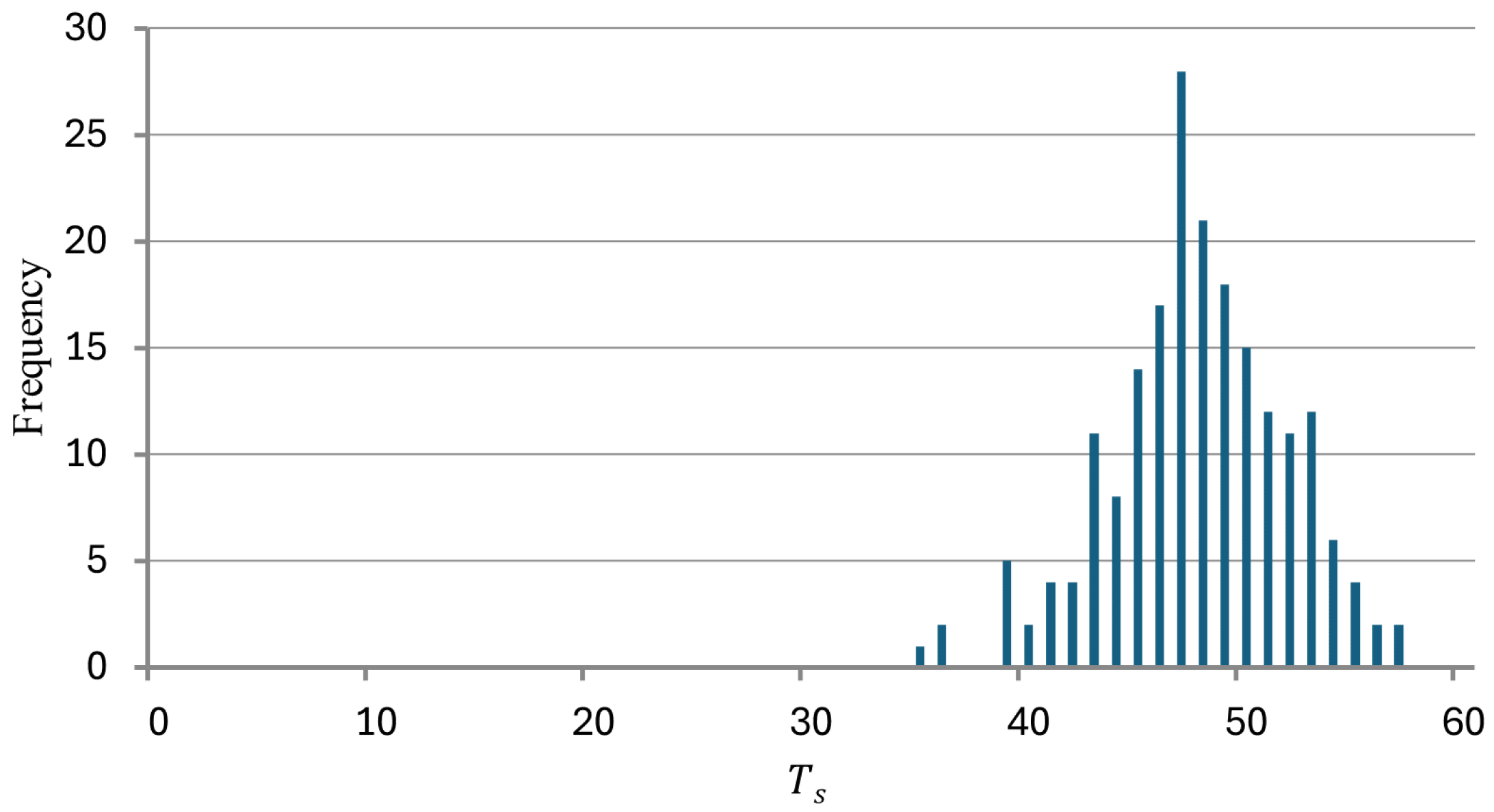
The event occurrence time T s of positive samples varied with each video clip and was manually determined. As shown in Figure 4, the distribution of T s is concentrated in the latter half of the video. The video clips included in the training dataset were given target labels y = ( y ( n ) , y ( p ) ) for the entire video clip, which were defined as y = ( 0 , 1 ) for positive and y = ( 1 , 0 ) for negative. The w a in Equation (3) was set experimentally to 1050, which is the length of the touchline of the field. Moreover, w 1 and w 2 in Equation (19) were set to 0.001 and 10, respectively, in order to balance the edge weights and loss values. In the training phase, the learning rate was initialized to 5 × 10 4 , and we employed Adam [57] and ReduceLROnPlateau as the optimizer and scheduler, respectively. The batch size was set to 16, and it was trained in 60 epochs.
To validate the effectiveness of the proposed model (PM) for shot prediction from soccer videos, we first conducted ablation studies that excluded the novelty from the PM. Specifically, we compared our model with the models without audio feature x t audio from graph nodes, xG from graph edge weights, and both of them, which were defined as Ablations1-3, respectively. We also compared with Ablation4, which employed a simple neural network instead of a BNN. Furthermore, we adopted the following models for the comparison.
DSA [58]:
This is a method for traffic accident prediction from dashcam videos. This model learns temporal relationships through RNN and the importance of detected objects in the video through Dynamic Spatial Attention (DSA).
DSTA [59]:
This is a video-based prediction model for traffic accidents, which uses GRU or LSTM to learn temporal relationships and Dynamic Spatial–Temporal Attention (DSTA) to learn the spatial and temporal importance of detected objects in the dashcam video.
ViViT [60]:
This is a video recognition model known as a Video Vision Transformer (ViViT), which learns spatial and temporal dynamics by tokenizing videos into a series of image frames or patches.
To the best of our knowledge, our previous studies [38,39,40,41] are the only ones that use visual information to predict the shot event occurrence in soccer matches. Therefore, we employed DSA and DSTA as comparative methods although they are video-based traffic accident prediction models that consider spatial–temporal relationships between objects in the video. In addition, since ViViT has the ability to classify the existence of events by recognizing various factors from the entire video image, it is considered to have the same ability as an accurate prediction of event occurrences. Hence, we adopted ViViT as a valid standard of comparison for event prediction methods.
In order to validate the prediction accuracy, we used Average Precision (AP) and F1-score (F1), which were defined as follows:
AP = t h ( Recall t h + 1 Recall t h ) Precision t h ,
F 1 t h = 2 × Recall t h × Precision t h Precision t h + Recall t h ,
where
Recall t h = TP t h TP t h + FN t h ,
Precision t h = TP t h TP t h + FP t h .
The prediction of event occurrence by the model is dependent on the threshold t h being exceeded. At the threshold t h , TP t h denotes the count of video clips correctly predicted as events, FP t h indicates the number of video clips incorrectly predicted as events, and FN t h refers to the number of video clips that were events but not predicted as events. Additionally, to measure the prediction earliness for positive samples, we evaluated event prediction performance with mean Time to Event (mTTE) calculated by the following equation:
mTTE = E [ TTE t h ] ,
TTE t h = max { T s t | β ( y t ) t h , 1 t T s } ,
where β ( · ) represents the sigmoid function. TTE is a common metric in prediction tasks and is used in various studies [39,58,59,61]. In this experiment, we verified the effectiveness of the proposed model in the above experimental settings.

3.2. Results and Discussion

3.2.1. Quantitative Results

Table 1 and Table 2 show the quantitative results for each method. Concretely, in Table 1, we show the prediction accuracy at different lengths of video clips, and the performance of PM is better than other models at almost all lengths of video clips. Note that in all video clips, the time T s of the shot occurrence is situated in the second half of the video clip. Compared with PM and Ablations1-3, we confirm that Ablation3 has the lowest and PM the highest performance when the length of video clips is long, that is, video clips including around the shot occurrence time T s . Since spectators cheered loudly at important moments, it is considered that the audio feature is effective for shot prediction. xG can reflect the importance of the player’s position in more detail, and thus, it is assumed that the introduction of xG into the graph edge weights is also useful by comparing PM with Ablation2. In comparison between PM and Ablation4, it is observed that although Ablation4 has a slightly higher AP for only the first half of the video, PM shows higher accuracy as the video length increases. From this result, we confirm that Ablation4 does not correctly capture the match situations, which indicates the effectiveness of using the BNN instead of a general neural network since the shot occurred in the second half of the video clip. Furthermore, the comparison of PM with DSA and DSTA shows that it is more effective in shot prediction in soccer matches than video-based shot prediction models, which achieved high performance in a different task. In the comparison between PM and ViViT, we confirm that PM significantly outperforms ViViT at all lengths of video clips. The above results show that PM achieves higher prediction accuracy than that of the state-of-the-art video prediction model. Here, DSA and DSTA achieve high prediction accuracy, although not as high as PM, in contrast to ViViT, which has a considerably less accurate performance than that of the other comparison methods. The reason for the low performance of ViViT could be attributed to the crucial difference that ViViT does not perform object detection. With the self-attention of the vision transformer, ViViT learns the interaction of each position in a video frame with the other positions. However, it is considered to be difficult to determine the focus points in a scouting video, which is captured from a bird’s-eye view of the field, without prior information. On the other hand, DSA, DSTA, and PM utilize object detection results to learn the extent to which each detected object is attributable to the prediction results. This difference may have affected the prediction accuracy. Moreover, PM utilizes a graph that introduces more detail on the importance of each player, which is assumed to be one of the factors behind its higher performance than that of DSA and DSTA.
Since the shot occurrence time T s is different for each video clip, we evaluate the prediction performance at time step T s . In Table 2, we present the prediction accuracy at time step T s and the prediction earliness for the positive sample. The values of Recall and Precision are determined at threshold t h in which F1 achieved the best performance. Note that in this experiment, ViViT, which classifies the existence of events from the entire video, is excluded from the comparison method since it is not possible to make predictions at each time step. As shown in Table 2, PM achieves the highest performance in all evaluation metrics than those of the other models. The comparison between PM and Ablations1–4 indicates the effectiveness of introducing each novelty in terms of prediction accuracy. DSA and DSTA also performed as well as the Ablation studies, although not as well as PM. Furthermore, we confirm that PM correctly predicts positive samples earlier than other models. Since PM has a high mTTE while ensuring high accuracy, it may be able to support players and coaching staff in making timely decisions based on the results. In summary, it is verified that PM is a quantitatively outstanding model for shot prediction tasks in soccer.

3.2.2. Qualitative Results

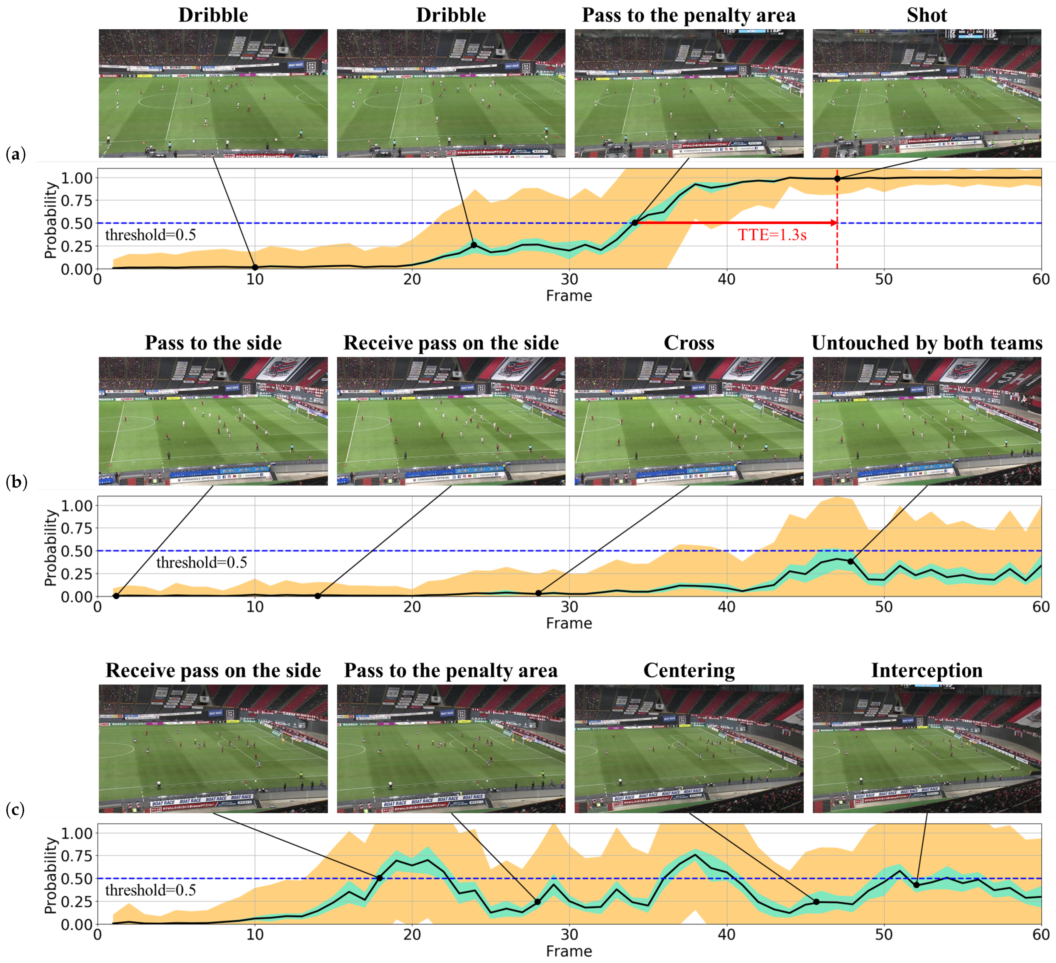
To qualitatively evaluate the prediction performance, visualized examples of the shot prediction results obtained by PM are shown in Figure 5. Each example result represents positive and negative outcomes of accurate predictions (true-positive and true-negative, respectively), followed by negative outcomes of incorrect predictions (false-positive). A threshold value t h = 0.5 was set to determine whether each prediction result was correct. In the figure of each example, several characteristic frames in the video clip are displayed at the top. For the bottom part of the figure, the prediction probability at each time step (black lines) and associated aleatoric and epistemic uncertainties (orange and cyan regions, respectively) are depicted. The larger region of each uncertainty at each time step indicates greater uncertainty regarding the prediction outcome. The true positive example shown in Figure 5a is a scene that includes the sequences of pass to near goal and shot, where the prediction probability increases rapidly after the pass into the penalty area and reaches the target threshold value 1.3 s before the shot moment. In this example, as the player dribbling approaches the penalty area gradually, the model provides a rising prediction probability while maintaining uncertainty. The fact that the model continues to offer significant uncertainty right up to the moment before the shot suggests that it recognizes the situation as ambiguous regarding whether the pass will succeed or not. The following example of a true negative shown in Figure 5b is a scene where a cross is made from the side but no one touches the ball. The prediction result does not exceed the threshold throughout the video, yet it suggests significant uncertainty. This indicates that while there are few attacking players near the goal, which leads to a low probability of a shot occurring, there is a potentially high possibility of it happening. Finally, we observe a false positive scenario where an attack from the side culminates in a centering attempt within the penalty area shown in Figure 5c. The predictive outcomes of this scene frequently reach the threshold in the video, accompanied by considerable uncertainty. Although this particular scene does not result in an actual shot, thus categorizing it as a negative instance in our study, it can arguably be considered a scene with a highly probable chance of leading to a shot or creating a shot opportunity. In a real soccer match, the shot opportunity often exists even in situations where the player does not choose the shot. This observation suggests that future research may need to reconsider the definitions within the dataset.

3.2.3. Limitations

There are some limitations to our study. First, a data-specific limitation is that it is challenging to identify the ball carrier in the scouting videos used in this study. This may lead to scenarios where a shot event occurs without the predicted probability reaching the threshold value. Next, there is a limitation on the number of datasets. In this experiment, we adopted ViViT as one of the comparison methods; however, its performance was lower compared to other methods. As one of the factors, it is considered that this may be the insufficient scale of the dataset. Since ViViT is a transformer-based model with a weak inductive bias, it has been reported that generalization performance is poor for small datasets and requires large datasets to achieve a high-performance model [62]. In this experiment, the total number of datasets was 400, which may not have been sufficient to achieve the same level of accuracy as our method. Furthermore, we applied the xG provided by MLS to the match data of the J1 League, which is a different league. Although xG for individual players and teams is provided in the J1 League and European leagues, the xG for each position on the field is not publicly available. In this study, we adopted the xG provided by MLS instead, considering that xG for each field position in soccer does not vary significantly across different leagues.

4. Conclusions

In this paper, we propose a model for multimodal shot prediction by utilizing spatial–temporal interactions between players in soccer videos. The proposed model constructs a graph that considers the relationship and importance of players with various audio-visual features acquired from the video as nodes. Then, we extract latent features from the graph based on GCRNN considering both spatial and temporal interactions. Finally, we predict the shot occurrence by using BNNs, which is a probabilistic deep-learning method. The BNN provides uncertainty about the prediction results and thus users can analyze and evaluate the results with high confidence. In experiments using video clips extracted from actual professional soccer league matches, our method achieved the highest accuracy in all evaluation metrics at and around the shot moment. Specifically, the results of an AP of 0.948 and an F1 score of 0.858 indicate that it is a high-performance prediction model, demonstrating its superiority. From the experiment, we confirmed the effectiveness of the novelty of our study, that is, the audio feature, and the xG for considering the importance based on players’ positions.
This approach is expected to improve predictive accuracy in diverse scenarios and environments. We also believe our shot prediction model can be easily adapted to other sports. Given that soccer is a sport with a large number of players and high degrees of freedom for each player, it is considered arguably more challenging than other sequential sports such as basketball and rugby. Therefore, as our model has successfully captured the more complex inter-player relationships in soccer, it is highly likely to provide accurate event predictions in similar competitive sports. Consequently, our model demonstrates significant applicability and potential benefits for a range of sports, underscoring its utility in diverse sporting contexts.

Author Contributions

Conceptualization, R.G., Y.M., K.M., T.O. and M.H.; methodology, R.G., Y.M., K.M. and T.O.; software, R.G.; validation, R.G.; data curation, R.G.; writing—original draft preparation, R.G.; writing—review and editing, Y.M., K.M., T.O. and M.H.; visualization, R.G.; funding acquisition, K.M., T.O. and M.H. All authors have read and agreed to the published version of the manuscript.

Funding

This work was partly supported by JSPS KAKENHI Grant Numbers JP21H03456 and JP23K11211.

Institutional Review Board Statement

Not applicable.

Informed Consent Statement

Not applicable.

Data Availability Statement

The soccer video dataset used in this study is a non-public dataset provided by Hokkaido Consadole Sapporo. The original contributions presented in the study are included in the article, further inquiries can be directed to the corresponding author.

Acknowledgments

In this research, we used the data provided by Consadole Sapporo.

Conflicts of Interest

The authors declare no conflicts of interest.

References

  1. Lord, F.; Pyne, D.B.; Welvaert, M.; Mara, J.K. Methods of performance analysis in team invasion sports: A systematic review. J. Sport. Sci. 2020, 38, 2338–2349. [Google Scholar] [CrossRef] [PubMed]
  2. Chmait, N.; Westerbeek, H. Artificial intelligence and machine learning in sport research: An introduction for non-data scientists. Front. Sport. Act. Living 2021, 3, 363. [Google Scholar] [CrossRef] [PubMed]
  3. Van Roy, M.; Yang, W.C.; De Raedt, L.; Davis, J. Analyzing learned Markov decision processes using model checking for providing tactical advice in professional soccer. In Proceedings of the International Joint Conference on Artificial Intelligence Workshop on AI for Sports Analytics, Virtual, 17–19 September 2021. [Google Scholar]
  4. Wang, J. Predictive Analysis of NBA Game Outcomes through Machine Learning. In Proceedings of the International Conference on Machine Learning and Machine Intelligence, Chongqing, China, 27–29 October 2023; pp. 46–55. [Google Scholar]
  5. Jones, R.N.; Greig, M.; Mawéné, Y.; Barrow, J.; Page, R.M. The influence of short-term fixture congestion on position specific match running performance and external loading patterns in English professional soccer. J. Sport. Sci. 2019, 37, 1338–1346. [Google Scholar] [CrossRef]
  6. Goes, F.; Meerhoff, L.; Bueno, M.; Rodrigues, D.; Moura, F.; Brink, M.; Elferink-Gemser, M.; Knobbe, A.; Cunha, S.; Torres, R.; et al. Unlocking the potential of big data to support tactical performance analysis in professional soccer: A systematic review. Eur. J. Sport Sci. 2021, 21, 481–496. [Google Scholar] [CrossRef] [PubMed]
  7. Forcher, L.; Altmann, S.; Forcher, L.; Jekauc, D.; Kempe, M. The use of player tracking data to analyze defensive play in professional soccer—A scoping review. Int. J. Sport. Sci. Coach. 2022, 17, 1567–1592. [Google Scholar] [CrossRef]
  8. Akenhead, R.; Nassis, G.P. Training load and player monitoring in high-level football: Current practice and perceptions. Int. J. Sport. Physiol. Perform. 2016, 11, 587–593. [Google Scholar] [CrossRef] [PubMed]
  9. Nobari, H.; Banoocy, N.K.; Oliveira, R.; Pérez-Gómez, J. Win, draw, or lose? Global positioning system-based variables’ effect on the match outcome: A full-season study on an Iranian professional soccer team. Sensors 2021, 21, 5695. [Google Scholar] [CrossRef] [PubMed]
  10. Pino-Ortega, J.; Oliva-Lozano, J.M.; Gantois, P.; Nakamura, F.Y.; Rico-Gonzalez, M. Comparison of the validity and reliability of local positioning systems against other tracking technologies in team sport: A systematic review. Proc. Inst. Mech. Eng. Part P J. Sport. Eng. Technol. 2022, 236, 73–82. [Google Scholar] [CrossRef]
  11. Anzer, G.; Bauer, P. A goal scoring probability model for shots based on synchronized positional and event data in football (soccer). Front. Sport. Act. Living 2021, 3, 624475. [Google Scholar] [CrossRef]
  12. Simpson, I.; Beal, R.J.; Locke, D.; Norman, T.J. Seq2Event: Learning the Language of Soccer using Transformer-based Match Event Prediction. In Proceedings of the the ACM International Conference on Special Interest Group on Knowledge Discovery and Data Mining, Washington, DC, USA, 14–18 August 2022; pp. 3898–3908. [Google Scholar]
  13. Pappalardo, L.; Cintia, P.; Rossi, A.; Massucco, E.; Ferragina, P.; Pedreschi, D.; Giannotti, F. A public data set of spatio-temporal match events in soccer competitions. Sci. Data 2019, 6, 236. [Google Scholar] [CrossRef]
  14. Biermann, H.; Theiner, J.; Bassek, M.; Raabe, D.; Memmert, D.; Ewerth, R. A unified taxonomy and multimodal dataset for events in invasion games. In Proceedings of the the ACM International Workshop on Multimedia Content Analysis in Sports, Chengdu, China, 20 October 2021; pp. 1–10. [Google Scholar]
  15. Lucey, P.; Bialkowski, A.; Monfort, M.; Carr, P.; Matthews, I. Quality vs quantity: Improved shot prediction in soccer using strategic features from spatiotemporal data. In Proceedings of the MIT Sloan Sports Analytics Conference, Boston, MA, USA, 28 February–1 March 2014; pp. 1–9. [Google Scholar]
  16. Decroos, T.; Van Haaren, J.; Dzyuba, V.; Davis, J. STARSS: A spatio-temporal action rating system for soccer. In Proceedings of the the ECML/PKDD Workshop on Machine Learning and Data Mining for Sports Analytics, Skopje, North Macedonia, 18 September 2017; Volume 1971, pp. 11–20. [Google Scholar]
  17. Power, P.; Ruiz, H.; Wei, X.; Lucey, P. Not all passes are created equal: Objectively measuring the risk and reward of passes in soccer from tracking data. In Proceedings of the the ACM International Conference on Special Interest Group on Knowledge Discovery and Data Mining, Halifax, NS, Canada, 13–17 August 2017; pp. 1605–1613. [Google Scholar]
  18. Spearman, W. Beyond expected goals. In Proceedings of the MIT Sloan Sports Analytics Conference, Boston, MA, USA, 23–24 February 2018; pp. 1–17. [Google Scholar]
  19. Liu, G.; Luo, Y.; Schulte, O.; Kharrat, T. Deep soccer analytics: Learning an action-value function for evaluating soccer players. Data Min. Knowl. Discov. 2020, 34, 1531–1559. [Google Scholar] [CrossRef]
  20. Vaswani, A.; Shazeer, N.; Parmar, N.; Uszkoreit, J.; Jones, L.; Gomez, A.N.; Kaiser, Ł.; Polosukhin, I. Attention is all you need. Adv. Neural Inf. Process. Syst. 2017, 30, 5998–6008. [Google Scholar]
  21. Naik, B.T.; Hashmi, M.F.; Bokde, N.D. A comprehensive review of computer vision in sports: Open issues, future trends and research directions. Appl. Sci. 2022, 12, 4429. [Google Scholar] [CrossRef]
  22. Deliege, A.; Cioppa, A.; Giancola, S.; Seikavandi, M.J.; Dueholm, J.V.; Nasrollahi, K.; Ghanem, B.; Moeslund, T.B.; Van Droogenbroeck, M. Soccernet-v2: A dataset and benchmarks for holistic understanding of broadcast soccer videos. In Proceedings of the the IEEE/CVF Conference on Computer Vision and Pattern Recognition Workshops, Virtual, 25 June 2021; pp. 4508–4519. [Google Scholar]
  23. Manafifard, M.; Ebadi, H.; Moghaddam, H.A. A survey on player tracking in soccer videos. Comput. Vis. Image Underst. 2017, 159, 19–46. [Google Scholar] [CrossRef]
  24. Hurault, S.; Ballester, C.; Haro, G. Self-supervised small soccer player detection and tracking. In Proceedings of the the International Workshop on Multimedia Content Analysis in Sports, Seattle, WA, USA, 16 October 2020; pp. 9–18. [Google Scholar]
  25. Cioppa, A.; Giancola, S.; Deliege, A.; Kang, L.; Zhou, X.; Cheng, Z.; Ghanem, B.; Van Droogenbroeck, M. Soccernet-tracking: Multiple object tracking dataset and benchmark in soccer videos. In Proceedings of the the IEEE/CVF Conference on Computer Vision and Pattern Recognition Workshops, New Orleans, LA, USA, 20 June 2022; pp. 3491–3502. [Google Scholar]
  26. Fu, X.; Huang, W.; Sun, Y.; Zhu, X.; Evans, J.; Song, X.; Geng, T.; He, S. A Novel Dataset for Multi-View Multi-Player Tracking in Soccer Scenarios. Appl. Sci. 2023, 13, 5361. [Google Scholar] [CrossRef]
  27. Khaustov, V.; Mozgovoy, M. Recognizing events in spatiotemporal soccer data. Appl. Sci. 2020, 10, 8046. [Google Scholar] [CrossRef]
  28. Alamuru, S.; Jain, S. Video event detection, classification and retrieval using ensemble feature selection. Clust. Comput. 2021, 24, 2995–3010. [Google Scholar] [CrossRef]
  29. Mahaseni, B.; Faizal, E.R.M.; Raj, R.G. Spotting football events using two-stream convolutional neural network and dilated recurrent neural network. IEEE Access 2021, 9, 61929–61942. [Google Scholar] [CrossRef]
  30. Nergård Rongved, O.A.; Stige, M.; Hicks, S.A.; Thambawita, V.L.; Midoglu, C.; Zouganeli, E.; Johansen, D.; Riegler, M.A.; Halvorsen, P. Automated event detection and classification in soccer: The potential of using multiple modalities. Mach. Learn. Knowl. Extr. 2021, 3, 1030–1054. [Google Scholar] [CrossRef]
  31. Sanabria, M.; Sherly; Precioso, F.; Menguy, T. A deep architecture for multimodal summarization of soccer games. In Proceedings of the International Workshop on Multimedia Content Analysis in Sports, Nice, France, 25 October 2019; pp. 16–24. [Google Scholar]
  32. Haruyama, T.; Takahashi, S.; Ogawa, T.; Haseyama, M. User-selectable event summarization in unedited raw soccer video via multimodal bidirectional LSTM. ITE Trans. Media Technol. Appl. 2021, 9, 42–53. [Google Scholar] [CrossRef]
  33. Honda, Y.; Kawakami, R.; Yoshihashi, R.; Kato, K.; Naemura, T. Pass Receiver Prediction in Soccer Using Video and Players’ Trajectories. In Proceedings of the the IEEE/CVF Conference on Computer Vision and Pattern Recognition Workshops, New Orleans, LA, USA, 20 June 2022; pp. 3503–3512. [Google Scholar]
  34. Fang, J.; Yeung, C.; Fujii, K. Foul prediction with estimated poses from soccer broadcast video. arXiv 2024, arXiv:2402.09650. [Google Scholar]
  35. Kipf, T.N.; Welling, M. Semi-supervised classification with graph convolutional networks. arXiv 2016, arXiv:1609.02907. [Google Scholar]
  36. Seo, Y.; Defferrard, M.; Vandergheynst, P.; Bresson, X. Structured sequence modeling with graph convolutional recurrent networks. In Proceedings of the International Conference on Neural Information Processing, Siem Reap, Cambodia, 13–16 December 2018; pp. 362–373. [Google Scholar]
  37. Neal, R.M. Bayesian Learning for Neural Networks; Springer Science & Business Media: New York, NY, USA, 2012; Volume 118. [Google Scholar]
  38. Goka, R.; Moroto, Y.; Maeda, K.; Ogawa, T.; Haseyama, M. Shoot event prediction from soccer videos by considering players’ spatio-temporal relations. In Proceedings of the the IEEE Global Conference on Consumer Electronics, Osaka, Japan, 18–21 October 2022; pp. 193–194. [Google Scholar]
  39. Goka, R.; Moroto, Y.; Maeda, K.; Ogawa, T.; Haseyama, M. Prediction of shooting events in soccer videos using complete bipartite graphs and players’ spatial-temporal relations. Sensors 2023, 23, 4506. [Google Scholar] [CrossRef] [PubMed]
  40. Goka, R.; Moroto, Y.; Maeda, K.; Ogawa, T.; Haseyama, M. Shoot Event Prediction in Soccer Considering Expected Goals Based on Players’ Positions. In Proceedings of the International Conference on Consumer Electronics-Taiwan (ICCE-Taiwan), PingTung, Taiwan, 17–19 July 2023; pp. 449–450. [Google Scholar]
  41. Goka, R.; Moroto, Y.; Maeda, K.; Ogawa, T.; Haseyama, M. Prediction of Shoot Events by Considering Spatio-temporal Relations of Multimodal Features. In Proceedings of the International Conference on Consumer Electronics-Taiwan (ICCE-Taiwan), PingTung, Taiwan, 17–19 July 2023; pp. 793–794. [Google Scholar]
  42. He, K.; Gkioxari, G.; Dollár, P.; Girshick, R. Mask r-cnn. In Proceedings of the the IEEE International Conference on Computer Vision, Venice, Italy, 22–29 October 2017; pp. 2961–2969. [Google Scholar]
  43. Sun, S.b.; Cui, R.y. Player classification algorithm based on digraph in soccer video. In Proceedings of the the IEEE Joint International Information Technology and Artificial Intelligence Conference, Chongqing, China, 20–21 December 2014; pp. 459–463. [Google Scholar]
  44. He, K.; Zhang, X.; Ren, S.; Sun, J. Deep residual learning for image recognition. In Proceedings of the the IEEE Conference on Computer Vision and Pattern Recognition, Las Vegas, NV, USA, 27–30 June 2016; pp. 770–778. [Google Scholar]
  45. Deng, J.; Dong, W.; Socher, R.; Li, L.J.; Li, K.; Fei-Fei, L. Imagenet: A large-scale hierarchical image database. In Proceedings of the the IEEE Conference on Computer Vision and Pattern Recognition, Miami, FL, USA, 20–25 June 2009; pp. 248–255. [Google Scholar]
  46. Araújo, D.; Davids, K. Team synergies in sport: Theory and measures. Front. Psychol. 2016, 7, 214015. [Google Scholar] [CrossRef] [PubMed]
  47. Pereira, L.R.; Lopes, R.J.; Louçã, J.; Araújo, D.; Ramos, J. The soccer game, bit by bit: An information-theoretic analysis. Chaos Solitons Fractals 2021, 152, 111356. [Google Scholar] [CrossRef]
  48. Ruiz, L.; Gama, F.; Ribeiro, A. Gated graph convolutional recurrent neural networks. In Proceedings of the the European Signal Processing Conference, A Coruña, Spain, 2–6 September 2009; pp. 1–5. [Google Scholar]
  49. Cui, Z.; Henrickson, K.; Ke, R.; Wang, Y. Traffic graph convolutional recurrent neural network: A deep learning framework for network-scale traffic learning and forecasting. IEEE Trans. Intell. Transp. Syst. 2019, 21, 4883–4894. [Google Scholar] [CrossRef]
  50. Elbasani, E.; Njimbouom, S.N.; Oh, T.J.; Kim, E.H.; Lee, H.; Kim, J.D. GCRNN: Graph convolutional recurrent neural network for compound–protein interaction prediction. BMC Bioinform. 2021, 22, 616. [Google Scholar] [CrossRef] [PubMed]
  51. Cho, K.; Van Merriënboer, B.; Gulcehre, C.; Bahdanau, D.; Bougares, F.; Schwenk, H.; Bengio, Y. Learning phrase representations using RNN encoder-decoder for statistical machine translation. arXiv 2014, arXiv:1406.1078. [Google Scholar]
  52. Hochreiter, S.; Schmidhuber, J. Long short-term memory. Neural Comput. 1997, 9, 1735–1780. [Google Scholar] [CrossRef]
  53. Wilson, A.G.; Izmailov, P. Bayesian deep learning and a probabilistic perspective of generalization. Adv. Neural Inf. Process. Syst. 2020, 33, 4697–4708. [Google Scholar]
  54. Izmailov, P.; Vikram, S.; Hoffman, M.D.; Wilson, A.G.G. What are Bayesian neural network posteriors really like? In Proceedings of the International Conference on Machine Learning, Virtual, 18–24 July 2021; pp. 4629–4640. [Google Scholar]
  55. Blundell, C.; Cornebise, J.; Kavukcuoglu, K.; Wierstra, D. Weight uncertainty in neural network. In Proceedings of the International Conference on Machine Learning, Lille, France, 6–11 July 2015; pp. 1613–1622. [Google Scholar]
  56. Kendall, A.; Gal, Y. What uncertainties do we need in bayesian deep learning for computer vision? Adv. Neural Inf. Process. Syst. 2017, 30, 5574–5584. [Google Scholar]
  57. Diederik, P.K.; Ba, J.L. Adam: A method for Stochastic Optimization. In Proceedings of the International Conference on Learning Representations, San Diego, CA, USA, 7–9 May 2015; pp. 1–15. [Google Scholar]
  58. Chan, F.H.; Chen, Y.T.; Xiang, Y.; Sun, M. Anticipating accidents in dashcam videos. In Proceedings of the the Asian Conference on Computer Vision, Taipei, Taiwan, 20–24 November 2016; pp. 136–153. [Google Scholar]
  59. Karim, M.M.; Li, Y.; Qin, R.; Yin, Z. A dynamic spatial-temporal attention network for early anticipation of traffic accidents. IEEE Trans. Intell. Transp. Syst. 2022, 23, 9590–9600. [Google Scholar] [CrossRef]
  60. Arnab, A.; Dehghani, M.; Heigold, G.; Sun, C.; Lučić, M.; Schmid, C. Vivit: A video vision transformer. In Proceedings of the the IEEE International Conference on Computer Vision, Montreal, BC, Canada, 11–17 October 2021; pp. 6836–6846. [Google Scholar]
  61. Neumann, L.; Zisserman, A.; Vedaldi, A. Future event prediction: If and when. In Proceedings of the the IEEE/CVF Conference on Computer Vision and Pattern Recognition Workshops, Long Beach, CA, USA, 16–17 June 2019; pp. 2935–2943. [Google Scholar]
  62. Raghu, M.; Unterthiner, T.; Kornblith, S.; Zhang, C.; Dosovitskiy, A. Do vision transformers see like convolutional neural networks? Adv. Neural Inf. Process. Syst. 2021, 34, 12116–12128. [Google Scholar]
Figure 1. An example of broadcast soccer videos and unedited soccer videos. To capture lengthy spatial–temporal relationships between players, the proposed method uses unedited soccer videos.
Applsci 14 04847 g001
Figure 2. Overview of the proposed method for multimodal shot prediction in soccer videos. In the proposed method, we adopt a graph with audio-visual features. We then obtain latent features that account for spatial-temporal relationships by using the GCRNN. Finally, we predict the probability of the shot occurrence as well as output the prediction uncertainty based on the BNN. A part of this figure is sourced from our previous paper [39].
Applsci 14 04847 g002
Figure 3. The expected goals (xG) used in the proposed model. Each zone is assigned a value based on the mean xG of shots taken within that zone in Major League Soccer.
Applsci 14 04847 g003
Figure 4. The distribution of T s in the positive samples.
Applsci 14 04847 g004
Figure 5. Examples of qualitative shot predictions when the threshold t h = 0.5 is set in PM. (a) true-positive and (b) true-negative examples of successful predictions and (c) false-positive example of incorrect predictions are shown in order. PM predicts the probability of shot occurrence at each time step (black line) in addition to estimating both corresponding aleatoric uncertainty (orange region) and epistemic uncertainty (cyan region).
Applsci 14 04847 g005
Table 1. Comparison of AP and F1 across varying video lengths for PM and other models. The time step t indicates the length of video clips from the beginning. The best performance for each length is shown in bold, and the second-best performance is underlined.
APF1
t = 10t = 20t = 30t = 40t = 50t = 60t = 10t = 20t = 30t = 40t = 50t = 60
Ablation10.8810.9210.9390.9440.9480.9470.7290.7820.8230.8480.8740.897
Ablation20.9120.9170.9340.9420.9580.9640.6720.7900.8290.8490.8600.854
Ablation30.9050.9230.9330.9400.9420.9420.6710.7500.7950.8230.8420.855
Ablation40.9150.9290.9370.9390.9420.9400.6010.7530.8000.8240.8310.832
DSA [58]0.8820.8800.8880.9290.9360.9320.7420.7770.8020.8180.8380.838
DSTA [59]0.9120.9230.9290.9280.9390.9460.6740.7630.8150.8290.8440.859
ViViT [60]0.7360.7440.7660.7700.7600.7550.6790.6820.6760.6790.6750.682
PM0.9130.9230.9380.9460.9590.9660.7570.8060.8250.8600.8760.891
Table 2. AP, Recall, Precision, F1, and mTTE for all methods except ViViT at time step T s . Note that Recall and Precision adopt the values at the threshold t h when F1 achieves the highest accuracy. Best and second-best performances are highlighted in bold and underlined, respectively.
APRecallPrecisionF1mTTE
Ablation10.9340.8070.8820.8393.46
Ablation20.9410.7810.8910.8243.63
Ablation30.9270.7970.8490.8013.46
Ablation40.9260.7660.8840.8163.61
DSA [58]0.9200.7860.8590.8203.71
DSTA [59]0.9250.8200.8560.8363.47
PM0.9480.8280.8960.8583.82
Disclaimer/Publisher’s Note: The statements, opinions and data contained in all publications are solely those of the individual author(s) and contributor(s) and not of MDPI and/or the editor(s). MDPI and/or the editor(s) disclaim responsibility for any injury to people or property resulting from any ideas, methods, instructions or products referred to in the content.