1. Introduction
High-pressure cooling turbine blades play a critical role in aero engines, operating under harsh conditions characterized by high temperature, high pressure, and high rotational speeds, which significantly influence the overall performance of the aero engine [
1]. During the service life of the blade, several disciplines such as aerodynamics, heat transfer, and structural strength are intricately interrelated and heavily influenced. Therefore, the design of the high-pressure cooling turbine blade is a typical multidisciplinary and complex work of system engineering. In high-temperature environments, conventional blade materials often struggle to maintain optimal performance. Employing high-temperature materials alongside thermal barrier coatings can enhance the thermal protection capabilities of blades to some extent. Furthermore, utilizing cooling mediums like low-temperature gas for heat exchange or employing insulation film cooling represent highly effective cooling strategies. However, the adoption of such cooling methods can lead to heightened string stress conditions [
2,
3]. Therefore, achieving an advanced turbine blade design requires comprehensive consideration of the interplay and synergistic effects between multiple disciplines, including aerodynamics, heat transfer, structure, and strength.
Traditional methods for designing a cooled turbine blade typically involve sequential analyses of aerodynamics, heat transfer, and structural strength. These methods often require multiple iterations to meet comprehensive performance criteria. However, relying on iterative design and verification, traditional methods have limited exploration capabilities for performance and struggle to identify optimal blade configurations. In contrast, Multidisciplinary Design Optimization (MDO) technology provides a solution by synchronizing considerations of various disciplines. It fully utilizes advanced optimization techniques to coordinate conflicts between discipline indicators in real time, thereby obtaining the most comprehensive blade design scheme [
4]. In recent years, MDO technology has found widespread application in turbine blade design optimization. For example, Li et al. [
5] conducted a multidisciplinary analysis of a cooling turbine blade using time-sequential conjugate heat transfer analysis and temperature–pressure interpolation strength analysis. Their study significantly improved the performance of the cooling turbine blade by integrating multiple disciplines and optimizing the blade design. Xiao et al. [
6] and Qian et al. [
7] established reliability models for a cooling turbine blade using fluid–thermal–structural coupled analysis methods. Compared to traditional models with failure-independent assumptions, such models demonstrate higher efficiency and accuracy. Yang et al. [
4] proposed a sensitivity analysis method for a cooling turbine blade considering surface thickness uncertainty, combining mesh deformation, neural network models, and multidisciplinary analysis. Li et al. [
8] established a multidisciplinary coupled analysis model for aerodynamics, heat transfer, and thermodynamics, effectively enhancing cooling performance through internal heat transfer reinforcement and external membrane cooling improvements. These studies offer compelling evidence supporting the feasibility and effectiveness of MDO–based optimization in engineering applications for cooled turbine blades, underscoring its substantial value.
The analysis of cooling turbine blades within a single discipline is already quite complex. When considering comprehensive optimization across multiple disciplines, challenges arise in terms of model complexity, computational complexity, and information exchange complexity. To address these challenges in practical engineering, surrogate models are often employed to replace intricate multidisciplinary system analyses. The surrogate model, which is also known as the metamodel, is one of the core technologies of MDO. Utilizing a limited amount of sample data generated by physical model tests and numerical analysis, it can establish mathematical models to improve computational efficiency under the premise of a certain accuracy level [
9]. In recent years, the surrogate model has received extensive research attention. Numerous surrogate models, including Polynomial Response Surface (PRS) models [
10], Kriging models [
11], Support Vector Regression (SVR) models [
12], Radial Basis Function (RBF) models [
13], and Artificial Neural Network models [
14], were proposed. Huang et al. [
15] proposed a new failure-related analysis strategy based on the Kriging model, conducting reliability assessments on high-pressure turbine rotors and enhancing computational efficiency. Qian et al. [
7] established a stress probability analysis model for aviation engine turbine rotors’ critical locations using response surface methods, demonstrating high efficiency and accuracy. Pietro et al. [
16] proposed a Multi-Fidelity Successive Response Surface (MF-SRS) model for collision testing, demonstrating superior accuracy and effectiveness in predictions when compared to the Successive Response Surface Method (SRSM). Xiao et al. [
17] introduced a machine learning-based method for predicting the lifespan of a turbine blade and predicted the remaining useful life through five start–stop cycles of a gas turbine. Xing et al. [
17] used a Kriging surrogate model to capture input data uncertainty and successfully obtained better performance variability in a robust optimization considering design uncertainties for pulse-corrected ballistic trajectories. Yang et al. [
4] constructed a neural network model for conducting sensitivity analysis on the multidisciplinary system of a turbine blade, reducing computational workload. The application of surrogate models in the optimization of a high-pressure cooling turbine blade addresses challenges posed by the complexity of multidisciplinary interactions, computational demands, and information exchange.
While the surrogate model offers various advantages, the suitability of different surrogate models for diverse problems varies. Given the absence of prior knowledge regarding the multidisciplinary design optimization of the cooling turbine blade, finding appropriate and highly precise surrogate models for practical engineering problems proves challenging. A common approach to address this challenge involves constructing an ensemble surrogate model, which integrates two or more independent surrogate models by introducing weight factors. The concept of the ensemble surrogate model traces back to the 1990s and has become a current research focus. In a study by Huang et al. [
18], a robust combination surrogate model was proposed through weighted combination, resulting in enhanced model accuracy. Yin et al. [
19] introduced a new weighting factor and established a new ensemble surrogate model named EM-MROWF, demonstrating superior performance compared to a single-surrogate model. Xue, et al. [
20] conducted a study on composite surrogate models from the aspects of selecting the model, calculating weight, and compensating residuals, proposing the OSF-TLPE composite surrogate model method and demonstrating its more flexible and reliable performance through testing. Combining the advantages of regression surrogate models and interpolation surrogate models, the authors of [
21] proposed a regression/interpolation combination surrogate model to leverage the global trend-fitting capability of regression surrogate models and the local accuracy prediction advantage of interpolation surrogate models, which can effectively enhance the accuracy and robustness of surrogate models. However, this surrogate model has not yet been applied in practical engineering optimization to demonstrate its utility.
This study focuses on the design optimization of a two-stage high-pressure turbine blade in a specific aeroengine. It establishes a parameterized model for a complex cooling blade and employs a regression/interpolation combination surrogate model to enhance efficiency in design optimization of the cooling turbine blade. The uniqueness of the proposed method lies in the establishment of a parameterized model that comprehensively considers the aerodynamic shape and internal cooling features of the cooling turbine blade. This parameterized model allows for the coupling of disciplines such as aerodynamics and strength in the design process, resulting in a comprehensive improvement in blade performance during the design optimization. Furthermore, this research offers certain advantages in improving the isentropic efficiency of the turbine stage under design conditions and enhancing the surface load distribution of the blade.
2. Turbine Stage Blade Model
The structure diagram of a two-stage high-pressure turbine rotor structure is shown in
Figure 1. The first-stage rotor blade is a cooling blade, which contains complex air-cooled structures such as partitions, turbulence ribs, internal cooling root segments, and trailing edge holes. Through the performance analysis of the initial scheme, it is known that the first-stage cooling turbine blade has a significant impact on the performance of the high-pressure turbine. Operating at high speeds in high-temperature gas environments, the blade endures complex forces such as centrifugal, aerodynamic, and temperature loads, leading to notable strength challenges. Therefore, the design of the cooling turbine blade needs to comprehensively consider multidisciplinary factors such as cooling efficiency and aerodynamics.
To enhance turbine performance, the emphasis is on the multidisciplinary design optimization of the cooling blade in the first-stage turbine. The aerodynamic performance of a high-pressure turbine is assessed based on four parameters: mass flow rate
, total expansion ratio
, 41-section efficiency
, and outlet flow angle
. Specifically, section 41 efficiency
is defined as follows:
In the formula, represents the adiabatic index of gas at section 41; represents the total power of the high-pressure turbine, units kW; represents the total gas temperature at the outlet of the first-stage guide vane of the high-pressure turbine, units K; and represents the universal gas constant.
To enhance turbine performance, this article considers the optimization of the 41-section efficiency as the objective function. The emphasis is on the multidisciplinary design optimization of the cooling blade in the first-stage turbine.
3. Multidisciplinary Design and Optimization of Turbine Stage Blade
This study focuses on optimizing the turbine blade. To enhance isentropic efficiency within the constraints of aerodynamic and strength performance, an efficient multidisciplinary integrated design optimization method for the cooling turbine blade is proposed. This method combines a parametric modeling approach for the cooling turbine blade with cooperative coupling characteristics, numerical simulation analysis methods from various disciplines, and a regression/interpolation combination surrogate model (
Figure 2). The specific steps involved in this method are as follows:
Select appropriate design variables and determine their ranges.
Select a suitable Design of Experiments (DOE) technique to generate a design matrix representing a set of sample points. Considering the precision required for the surrogate model and the time constraints for aerodynamic and strength analysis, an initial set of 200 sample points was generated using the “lhsdesign” program in MATLAB (v.2011).
Employ the blade modeling approach outlined in
Section 3.1.1. A custom MATLAB (v.2011) program was utilized to produce blade profile curves for the tip, middle, and root sections of the first-stage rotor blade across the 200 samples from step (2). The scatter coordinates of these blade profile curves were exported in various formats to facilitate blade modeling within the aerodynamic domain and parameterized modeling of the cooling blade within the structural domain.
Utilize the parameterized modeling approach outlined in
Section 3.1.2 for the cooling blade. The UG macro command was employed to automatically generate the geometric model of the first-stage rotor blade for strength analysis across the 200 samples from step (2).
Use the aerodynamic analysis method detailed in
Section 3.2.1. A high-fidelity Computational Fluid Dynamics (CFD) simulation of the two-stage high-pressure turbine blade was conducted using ANSYS (2020 R1) CFX software across all samples. Subsequently, pertinent response parameters were extracted, namely
W41,
π,
η and α.
Employ the strength analysis method outlined in
Section 3.2.2. Finite element simulation analyses of the first-stage rotor blade were conducted across all samples using the APDL language within ANSYS (2020 R1) software. Subsequently, the relevant response parameters were extracted.
Combine sampling points with their respective response parameters to create the initial sample database.
Utilizing existing sample data, integrate the advantages of two different surrogate models, and construct a regression/interpolation combination surrogate model.
Select a suitable optimization algorithm for the optimization process. The optimization objectives and constraint parameters are approximated by the regression/interpolation combination surrogate model developed in step (8). Details of the constructed optimization model will be presented in
Section 3.4. A Genetic Algorithm (GA) was employed to solve the constrained optimization problem in this study.
Generate a new blade profile curve for the tip, middle, and root sections of the first-stage rotor blade based on the optimized design obtained in step (9). Output the scatter coordinates of the curve in different formats.
Employ UG macro commands to automatically generate the geometric models of the first-stage rotor blade for the new design scheme obtained in step (9).
Utilizing ANSYS CFX software, conduct high-fidelity CFD simulations for the two-stage high-pressure turbine blade based on the new design scheme. Then extract relevant response parameters.
Using the APDL language within ANSYS (2020 R1) software, conduct finite element simulation analyses of the first-stage rotor blade for the new design scheme. Extract relevant response parameters σeq,max.
Verify the fulfillment of convergence criteria. If satisfied, conclude the loop and acquire an improvement plan. If not satisfied, update the existing sample database and iterate through steps (8) to (14) again.
3.1. Parameterized Modeling Method of Cooling Turbine Blade
3.1.1. Blade Shape Parameterization
The planar cascade design forms the fundamental basis of the turbine blade design. Its objective is to shape the aerodynamics of the blade across various radial cross-sections and provide blade profile data essential for the radial stacking of the blade. Typically, turbine blade cascades comprise four profiles: the leading edge, trailing edge, blade suction surface, and blade pressure surface. While the leading and trailing edge profiles are commonly represented by circular arc curves, the blade suction and pressure surface curves tend to be more complex. To ensure the smoothness of the blade profiles, this study employs a direct analytical approach for shaping the flat blade grid.
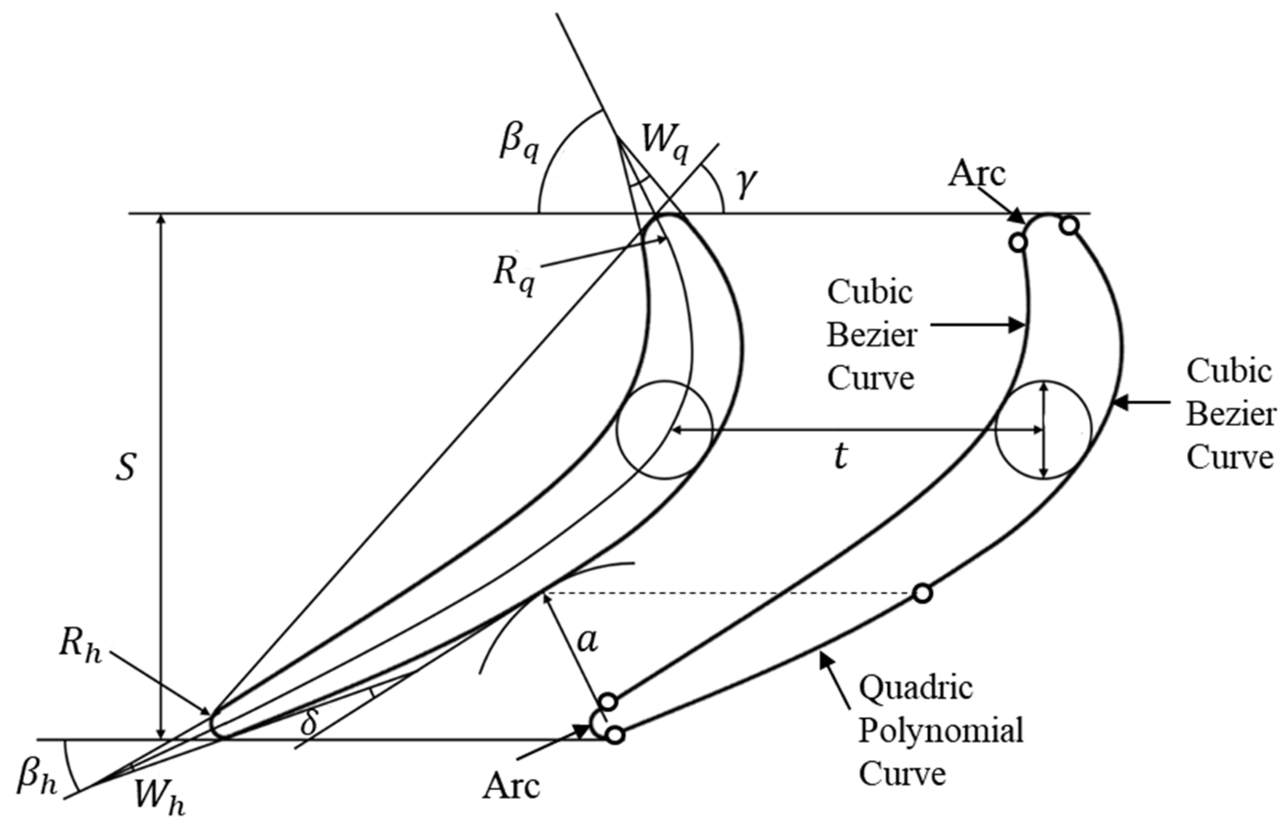
Figure 3 illustrates the geometric parameters and key control points necessary for the adopted planar cascade modeling method. Based on 11 primary parameters—including the leading edge radius
, trailing edge radius
, inlet geometric angles
, outlet geometric angles
, inlet wedge angles
, outlet wedge angles
, turning angle
, blade stagger angle
, axial chord length
, throat width
, and blade pitch
—the positions of the five blade control points and their tangent directions can be uniquely determined (as shown in
Figure 3). With the positions of control points and tangent directions established, a third-order Bezier curve is employed to delineate the entire blade bowl profile and the frontal section profile at the back of the blade. Additionally, a fourth-order polynomial curve is utilized to depict the rear section profile, ensuring curvature continuity between the two curves at the throat point and mitigating aerodynamic losses arising from curve connections.
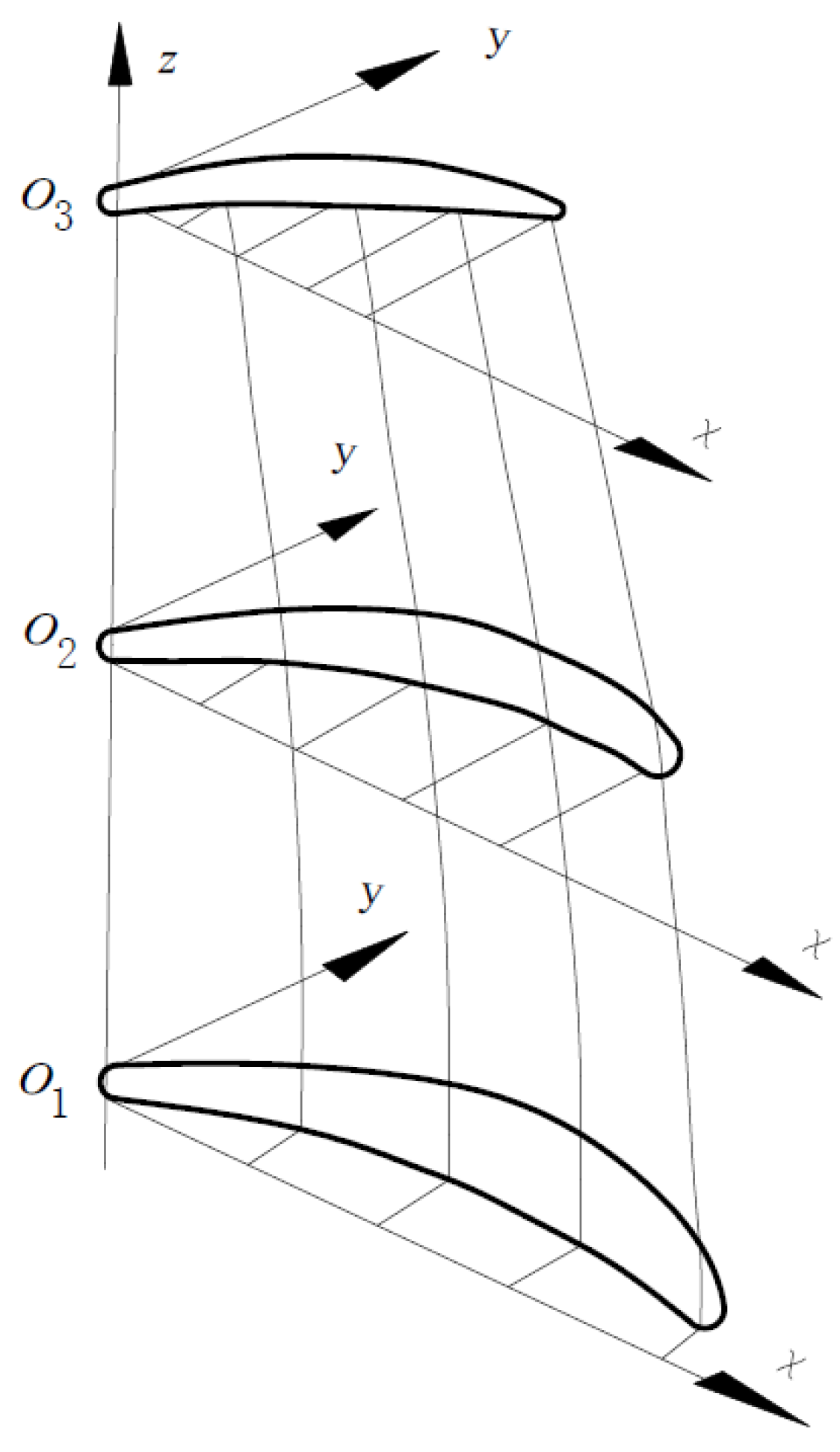
Radial stacking of the blade aims to interpolate blade profiles across various radial sections, utilizing the design output from the planar cascade shape. This interpolation is used to perform radial stacking according to the chosen stacking law, thereby achieving a smoothly contoured blade body. Given that typical aerodynamic parameters of the turbine blade exhibit linear deviation along the blade height, a parabolic stacking law was employed to shape the blade body after obtaining profile data at the root, middle, and tip sections, as illustrated in
Figure 4.
3.1.2. Parametric Modeling of Cooling Characteristics
MDO requires the automatic updating of geometric models based on design parameters. This involves collaboratively integrating feature parameterization modeling for both blade air cooling characteristics and adjustments to blade shape.
To mitigate the bending moment caused by centrifugal force in the turbine rotor blade, it is essential to distribute the center of gravity of the blade section radially along its height. The incorporation of typical cooling features can significantly alter the center of gravity of the blade section. Therefore, it is necessary to develop a parametric model for the hollow blade with variable wall thickness, which allows for swift adjustment of the center of gravity by altering the wall thickness distribution. Variable wall thickness encompasses three aspects: (1) variation of wall thickness dependent on radial height, (2) variation of wall thickness in the axial direction, and (3) independent variation of thickness at the pressure and suction sides. To accomplish this, the parametric modeling approach for the blade cavity in this study includes the following steps:
Establish eight feature control points on the suction side profile, as illustrated in
Figure 5.
Determine the corresponding eight feature control points on the pressure side profile using geometric constraints based on inscribed circles at the feature control points.
Connect the corresponding feature control points on the pressure and suction side profile and control the wall thickness at the pressure and suction sides using line length percentages.
Ensuring cavity smoothness by incorporating the wall thickness values at the first, third, and eighth feature control points on the pressure and suction sides as variables. These values are then interpolated through quadratic interpolation to determine the wall thickness at the remaining feature control points.
Generate cavity curves on the pressure and suction using spline curves.
Repeat steps (1) to (5) to obtain the cavity design sections corresponding to the external blade shape at the root, middle, and tip. The blade cavity is obtained using the UG curve group command.
Expanding on the parametric model for the variable wall thickness hollow blade, a feature-based parametric modeling approach was adopted to separately design the leading edge and dovetail structures. Subsequently, typical cooling features, including baffles, turbulence ribs, internal cooling root segments, and trailing edge holes, were iteratively enhanced. Through this iterative process, a comprehensive parametric model for the cooling blade was developed, as illustrated in
Figure 6.
3.2. Subject Analysis of Turbine Stage Blade
3.2.1. Fidelity CFD Simulation Analysis
The ANSYS (2020 R1) CFX software, renowned for its high accuracy in solving turbine aerodynamic problems and demonstrating robust convergence stability, was employed in this study for high-fidelity CFD simulation [
22]. It resolved the steady-state compressible Reynolds Average Navier-Stokes (RANS) equation via the finite volume method, utilizing the Shear Stress Transport (SST) turbulence model to simulate the viscous term. Each blade row’s rotor static interface was configured as “Stage”, and the Advance Scheme and Turbulence Numbers were set to “High Resolution”.
A single blade channel served as the computational domain, with periodic boundary conditions applied on both sides. The flow working fluid in the main channel of this article was gas, with a molar mass of 28.94 kg/kmol. The Dynamic Viscosity was set to 1.831 × 10⁻⁵ kg/(m * s). The inlet boundary conditions encompassed total temperature, total pressure, and airflow angle direction. Inlet turbulence was moderated at 5%, while outlet boundary conditions were specified in terms of average static pressure. Solid wall boundaries were treated as adiabatic and no slip wall.
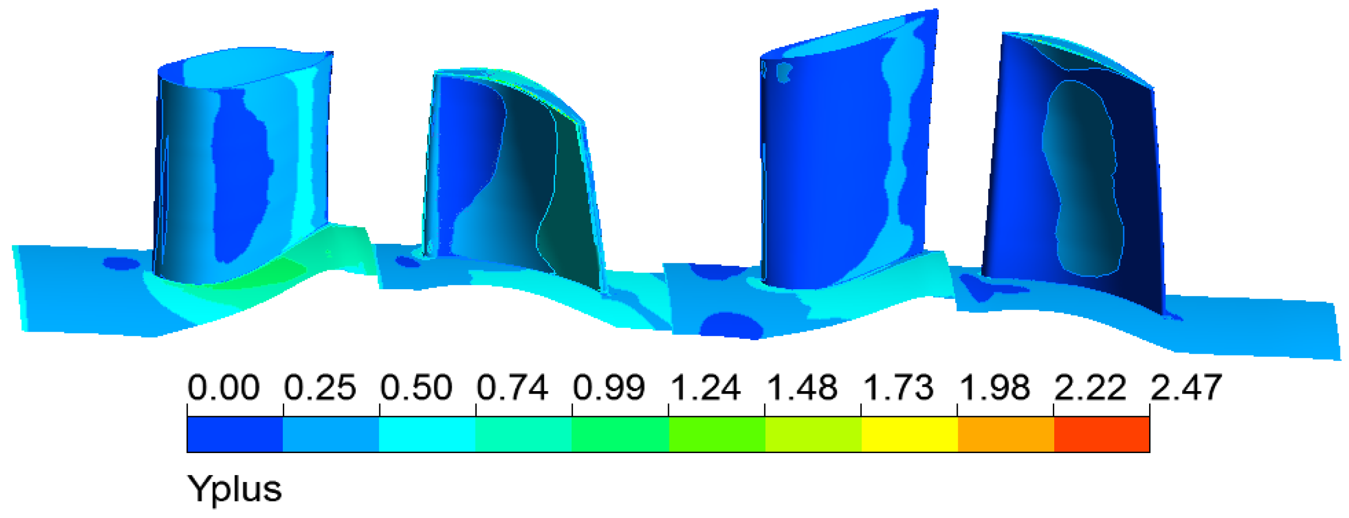
Grid partitioning was performed using ANSYS (2020 R1) TurboGrid software, with the grid topology structure set to ATM Optimized. The total number of grids and the number of spanwise grids in the meridian channel were separately adjusted to regulate overall grid quality, ensuring a value less than or approximately equal to 1 (as depicted in
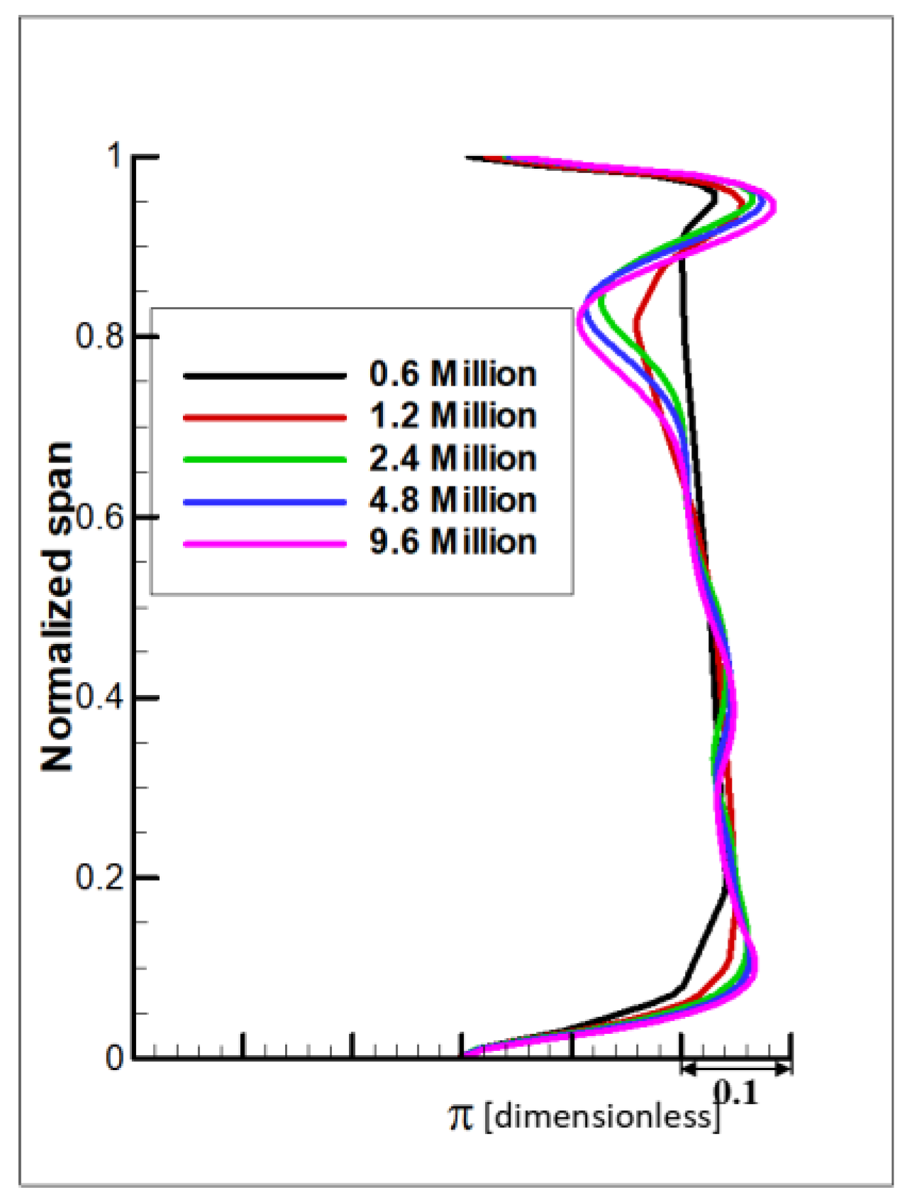
Figure 7) to meet the SST turbulence model grid quality requirements. The rotor blade tip clearance was set at 0.3 mm, with over 13 grid layers at the clearance to capture flow details. To verify grid independence and mitigate the flow field calculation result dependency on grid accuracy, five grid partitioning schemes with varying grid numbers were established: 0.6 million, 1.2 million, 2.4 million, 4.8 million, and 9.6 million.
Figure 8 illustrates the radial distribution of the total expansion ratio of high-pressure turbines across these five grid schemes, revealing the following: (1) A trend towards consistent radial distribution with increasing grid numbers. (2) When the grid number reaches 2.4 million, the impact on flow field calculation results is relatively minor, indicating grid independence.
Considering both computational accuracy and efficiency, this paper ultimately selected a grid partitioning scheme comprising 2.4 million grids (illustrated in
Figure 9) for numerical calculations and optimization design.
3.2.2. Strength Analysis of Rotor Blade Considering Internal Cooling Structure
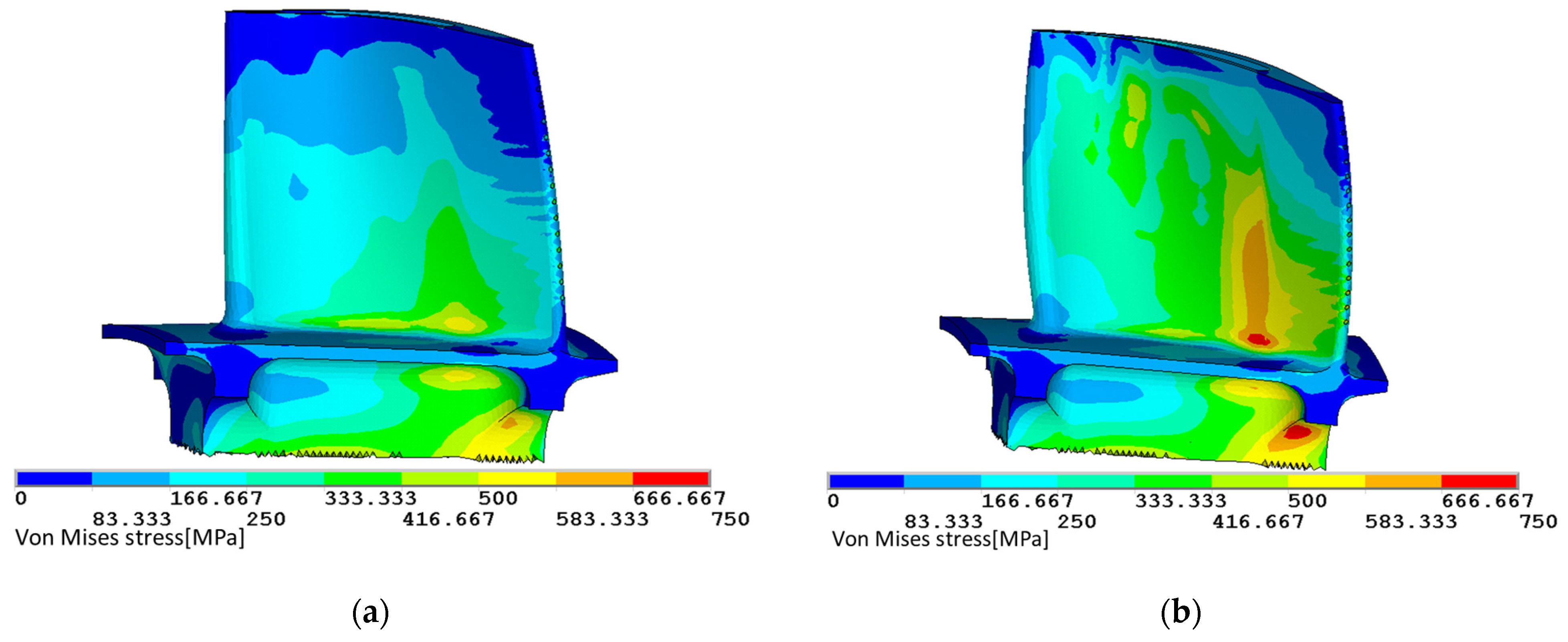
The cooling turbine blade in service should withstand significant mechanical strain caused by centrifugal loads and coupled with complex loads such as geometric stress concentration, airflow pressure, and temperature load. The stress state is extremely complex, so it is necessary to analyze the stress distribution of the turbine blade and evaluate the strength through the finite element method, providing a basis for the MDO of the blade.
This section analyzes the stress on the first-stage rotor blade with linear elastic finite element analysis by ANSYS. The unit type is 10 nodes tetrahedral unit SOLID187. The temperature field distribution of the cooling turbine blade affects both thermal stress and material mechanical properties, thereby affecting blade strength. The use of a three-dimensional high-fidelity numerical simulation for the flow heat coupling calculation of the blade needs a long cycle, resulting in low efficiency in multidisciplinary design optimization iterations. Therefore, in the optimization analysis of this study, a simplified temperature field was adopted, which is to calculate the average temperature of the blade along the radial section and obtain the distribution of blade temperature along the radial direction.
Figure 10 shows the grid and temperature field used in the optimized design.
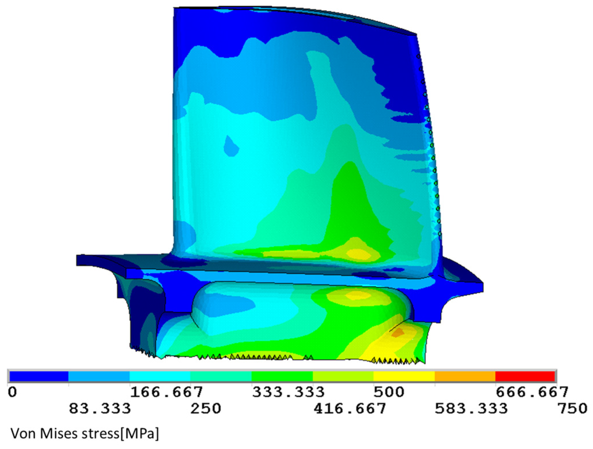
Based on a simplified temperature field and applying loads such as rotational speed, the equivalent stress cloud map of the blade is analyzed, as shown in
Figure 11.
3.3. Regression/Interpolation Combination Surrogate Model
Generally, different individual surrogate models are suitable for different types of prediction tasks. For instance, the regression surrogate model captures the global trend effectively while the interpolation surrogate model exhibits higher local accuracy at sampling points [
23,
24]. To amalgamate the strengths of common individual surrogate models and bolster their accuracy and robustness, the authors introduced a regression/interpolation combination surrogate model [
21]. This model integrates the advantages of regression and interpolation surrogate models.
The PRS model is one of the most widely used regression surrogate models in MDO. It primarily employs simple low-order polynomials (usually first- or second-order polynomials) to approximate relationships between weak nonlinear responses and variables in actual physical systems. This approach offers notable advantages in terms of modeling efficiency and transparency [
25]. The RBF model serves as an interpolation surrogate model that transforms multidimensional prediction problems into one-dimensional problems by considering Euclidean distance as a variable. It demonstrates excellent flexibility, high computational efficiency, and outstanding adaptability to high-dimensional nonlinear problems [
26]. Therefore, this paper selects the PRS model and RBF model to construct an ensemble surrogate model named the regression/interpolation combination surrogate model.
3.3.1. Construct a Regression Surrogate Model
The second-order PRS model is chosen as the regression surrogate model. The PRS can be written as
where
denotes the second-order polynomial response surface model,
denotes a polynomial basis-function vector, and
denotes a coefficient vector.
3.3.2. Update Training Sample Information
By using Equation (2), the responses of the established PRS
at the initial sampling locations
can be calculated. The updated PRS training dataset can be obtained accordingly:
3.3.3. Construct the Interpolation Class Surrogate Model
The RBF model, by choosing the multiquadric-form basis function, is selected as the interpolation-type surrogate model. The general form of the RBF can be expressed as [
13]
where
denotes an interpolation coefficient,
denotes a radially symmetric basis function, and
denotes the distance between points
and
.
The multiquadric-form basis function can be expressed as .
By using the given training dataset
, it is easy to calculate the interpolation coefficient using the following equation:
where
After choosing the multiquadric-form basis function, the RBFM (RBF with multiquadric-form basis function, ) can be constructed to approximate the actual model by substituting and into Equation (4). The coefficient can be calculated using Equation (5).
Moreover, by choosing the multiquadric-form basis function, a model can be established to approximate , the deviation function of the PRS, which is obtained by subtracting the PRS() from the actual model. The coefficient of can be calculated by substituting the updated training dataset of the PRS into Equation (5).
3.3.4. Construct a Composite Surrogate Model
By adding the established
and
together, R/ICSM(
) can be subsequently constructed as follows:
The established R/ICSM can be used to predict the response at any point within the design space by using Equation (7).
3.4. Optimization Model Description
This article aims to enhance the efficiency of the turbine 41 cross-section through multidisciplinary design optimization of the cooling blade in the first-stage turbine. Drawing on previous design experience, this study identified design variables, including the radius at the leading edge radius , inlet geometric angles , outlet geometric angle , inlet wedge angles , turning angle , blade stagger angle , and axial chord length , for each section. It is crucial to mention that, due to installation considerations involving blade and tenons, the axial chord length of the blade root section was excluded from the scope of design variables. To mitigate potential adverse effects on downstream components caused by the optimization of the high-pressure turbine blade, it is imperative to improve the efficiency of the high-pressure turbine 41 section while maintaining a constant gas flow rate and total expansion ratio . Additionally, it is essential to ensure that the outlet flow angle α of the high-pressure turbine falls within a reasonable range. Simultaneously, it is imperative to ensure that the maximum von Mises stress on the blade remains below a specified threshold to guarantee the blade’s safe and reliable operation. Therefore, parameters , , α and were selected as constraint parameters.
In summary, the optimization model is represented by the following formula:
In the formula, represents a small constant, denotes the design variable vector, and and denote the lower and upper limits of the design variable , respectively. Subscripts 1, 2, and 3 denote the blade tip section, blade center section, and blade root section, respectively, while the subscript denotes the relevant parameters of the initial scheme of the high-pressure turbine.


 and
and 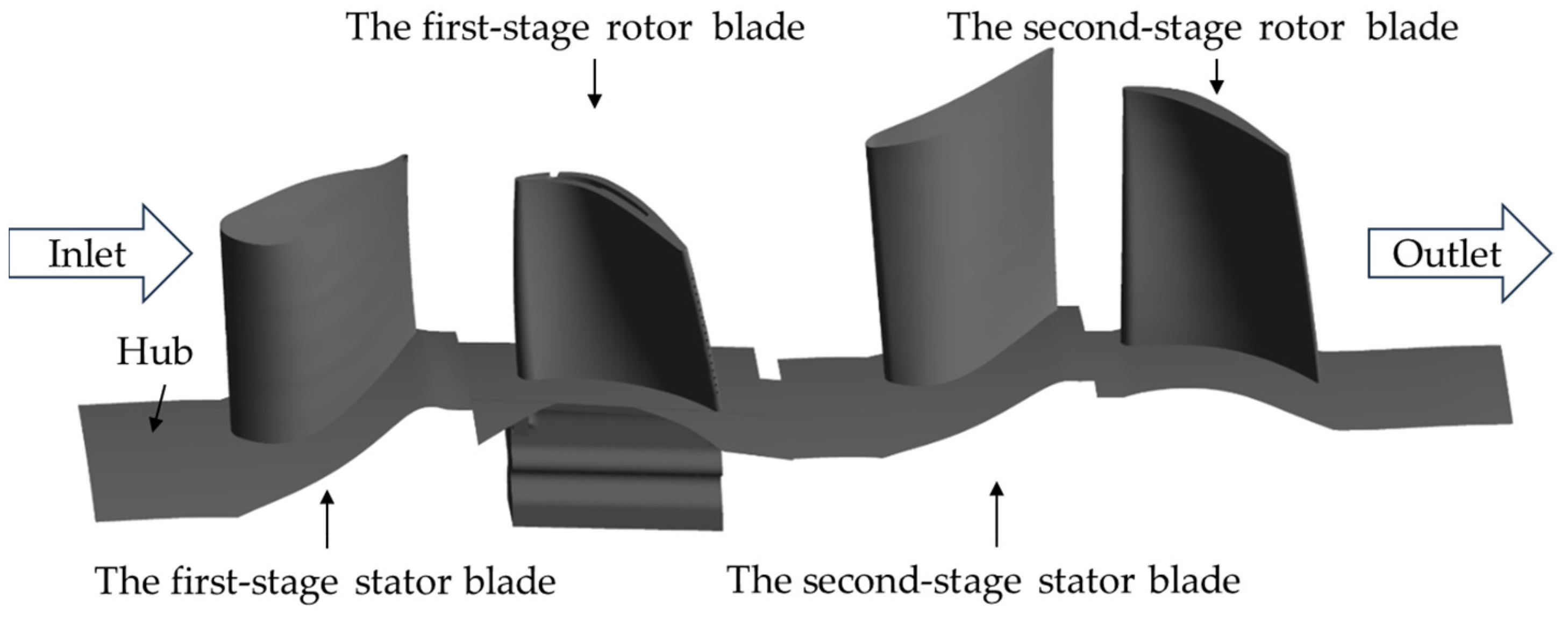


