Fixed-Point Iteration Method for Uncertain Parameters in Dynamic Response of Systems with Viscoelastic Elements

Abstract

The paper presents a method for determining the dynamic response of systems containing viscoelastic damping elements with uncertain design parameters. A viscoelastic material is characterized using classical and fractional rheological models. The assumption is made that the lower and upper bounds of the uncertain parameters are known and represented as interval values, which are then subjected to interval arithmetic operations. The equations of motion are transformed into the frequency domain using Laplace transformation. To evaluate the uncertain dynamic response, the frequency response function is determined by transforming the equations of motion into a system of linear interval equations. Nevertheless, direct interval arithmetic often leads to significant overestimation. To address this issue, this paper employs the element-by-element technique along with a specific transformation to minimize redundancy. The system of interval equations obtained is solved iteratively using the fixed-point iteration method. As demonstrated in the examples, this method, which combines the iterative solving of interval equations with the proposed technique of equation formulation, enables a solution to be found rapidly and significantly reduces overestimation. Notably, this approach has been applied to systems containing viscoelastic elements for the first time. Additionally, the proposed notation accommodates both parallel and series configurations of damping elements and springs within rheological models.

1. Introduction

The process of designing and analyzing structures involves the consideration of a wide range of factors that can influence their behavior under dynamic conditions. Uncertainties concerning design parameters, materials, production processes, and environmental conditions are significant factors that can greatly impact the safety, reliability, and performance of structures. Traditional approaches to dynamic structural analysis often overlook these uncertainties associated with design parameters, leading to inaccuracies in predicting structural behavior under real operating conditions. Therefore, addressing uncertainties is a crucial aspect of modern design processes.

There are some main approaches to incorporating uncertainties associated with design parameters. The first is the probabilistic approach, which assumes that uncertainties in design parameters are modeled using statistical parameters. This allows for the determination of the probability of various scenarios, and examples of its application can be found in works by Ghanem and Spanos [1], Capillon et al. [2], as well as Wang et al. [3], including research within the context of structures with viscoelastic elements. However, many cases present challenges such as insufficient statistical data or difficulties in precisely determining probability distributions for all design parameters. In such cases, the second approach, involving interval analysis, is utilized. Here, design parameters are defined by interval values. This article employs interval analysis to investigate the impact of uncertainties in design parameters on the dynamic response of structures.

One of the simplest tools that can be applied is the Monte Carlo method and the vertex method. The Monte Carlo method involves repeatedly sampling from specified intervals for individual design parameters and then conducting an analysis for each sample (Jiang et al. [4]). While effective, its main drawback is the high computational cost, especially for complex construction models and a large number of parameters. On the other hand, the vertex method relies on representing intervals using vertices and finding solutions for all their combinations (Qiu et al. in [5,6]). This method is also time-consuming, which is why, in recent decades, efforts have been focused on finding other methods to reduce the computational burden.

Chen et al. in [7,8] and Yang in [9] presented a method for computing uncertain eigenvalues of systems with interval parameters. They proposed the utilization of matrix perturbation theory and interval extension theory. Both undamped and damped cases were considered. A similar approach was applied in [10] by Qiu and Wang but for determining the dynamic response of structures. The authors also conducted a comparison of the obtained results with the probabilistic approach, based on both mathematical proofs and numerical simulations. The range of obtained results encompassed those obtained by the probabilistic method.

An alternative to perturbational methods has been presented in [11] by Xia et al. The authors introduced a method based on the vertex method, which was applied to the first-order deviation of dynamic response. They demonstrated that this proposed method reduces overestimation and is also more accurate than perturbational methods. However, it is worth noting that second-order components in the equations of motion were omitted in their considerations; hence, the method may not be suitable when parameter variability is high.

Sim et al. in [12] and Moens and Vandepitte in [13] applied modal interval analysis, combining modal analysis and interval calculus. The authors presented a method for finding eigenfrequencies, modal shapes, and frequency response functions (FRFs).

Yaowen et al. in [14] determined the frequency response function for systems with uncertain parameters using the Laplace transform. This transformation converted dynamic equilibrium equations into a linear system of algebraic equations. The authors also applied the element-by-element technique, which significantly reduced overestimation resulting from the dependencies between interval parameters. However, this method is only suitable for handling small uncertainties.

The procedure for deriving approximate explicit values of FRFs for systems with uncertainties was presented in [15] by Muscolino et al. The effectiveness of the Rational Series Expansion in estimating the lower and upper bounds of FRF values was demonstrated. The proposed method also effectively mitigates overestimations.

In the work [16] written by Wei et al., an approach based on two-dimensional Chebyshev polynomials was introduced for estimating the dynamic response of structures with interval uncertainties. The authors utilized the decomposition of the dynamic response function into univariate and bivariate functions and fitted them using Chebyshev polynomials. This approach facilitates the transformation of the dynamic analysis of nonlinear systems with uncertain parameters into solving simpler one-dimensional and two-dimensional equations.

In studies concerning uncertain design parameters, obtaining the response of structures, particularly in dynamic problems, is greatly facilitated by expanding the sought value into a Taylor series around the central value. This approach utilizes the sensitivities of the sought function with respect to changes in uncertain design parameters. In the work [17], Qiu et al. applied this approach to estimate the dynamic response of damped systems. In reference [18] written by Chen et al., it was shown that using a second-order Taylor series enables the accurate estimation of structural responses even with large uncertainties, although the focus was on undamped systems. In reference [19], Fujita and Takewaki proposed the identification of critical combinations of uncertain parameters by maximizing the objective function through second-order Taylor series expansion. The structure under consideration included dampers, with uncertain parameters extending to damper characteristics as well. Additionally, in the works [20] by Łasecka-Plura and Lewandowski and [21] by Łasecka-Plura, structures featuring viscoelastic elements were analyzed. These studies presented algorithms that notably reduced the number of combinations needed to determine the lower and upper bounds of the sought dynamic response of the structure.

One method that enables the incorporation of uncertainties in design parameters is stochastic analysis (Kamiński et al. in [22,23]). This approach, particularly when parameters are described as interval numbers, was applied by Muscolino and Sofi in [24] using affine arithmetic. This application helped reduce the overestimation of the determined structural response. Instead, Wang et al., in [25], introduced a hybrid approach where the boundaries of probabilistic characteristics are determined through interval arithmetic. Additionally, an approach utilizing Chebyshev polynomials to solve problems with multiple uncertain variables was introduced.

The authors also address scenarios where the analyzed systems are described using mixed random and interval parameters. In reference [26] by Zhao, a method was proposed to determine the lower and upper bounds of the mean value and standard deviation assuming the presence of mixed uncertain parameters. This method is based on expanding a series of random and interval quantities with respect to uncertain parameters. A comparison with the Monte Carlo method was also conducted, demonstrating a significant reduction in computational costs. In reference [27], Feng et al. considered the time response of structures and proposed a hybrid model combining generalized polynomial chaos theory and the Legendre metamodel method. On the other hand, Zhao et al., in refence [28], presented a method based on genetic algorithms for computing optimization problems with hybrid uncertain parameters.

Interval analysis finds broad application when dealing with uncertain design parameters, extending to other problems related to the analysis of structural behavior under dynamic loads. In [29] by Sofi et al., it was applied to analyze the reliability of systems with viscoelastic dampers; in [30] by Wang et al., it was applied to assess the reliability of systems with active vibration control; and in [31], Fang and Huang utilized it in the analysis of structural damage detection involving various types of uncertainties.

Uncertainty consideration is also discussed in the context of optimization. In [32], Wang et al. proposed a method for manipulator trajectory control, taking into account uncertainties. This method utilizes a non-probabilistic uncertainty quantification approach, ensuring precision and effectiveness in evaluating system response. On the other hand, in [33], Wang et al. presented topology optimization for continuous structures, considering uncertainties and time-dependent reliability. It employs a parameterized level set method based on reliability criteria. Meanwhile, in [34], Liu and Wang introduced a hybrid optimization method for vibration controller design, considering mixed uncertainties. Uncertainties are treated as intervals and fuzzy models.

As part of the analysis of systems with uncertain parameters, the issue of interval sensitivity is also considered, where the influence of individual uncertain input parameters on the range of obtained results is determined. In [35], Moens and Vandepitte demonstrated a procedure for determining the sensitivity of frequency response function bounds.

This article analyzes viscoelastically damped systems with uncertain design parameters. Methods for incorporating uncertainties in such systems, as described in the literature, can be divided into probabilistic methods, methods based on fuzzy theory, and methods where uncertainties are modeled as interval numbers. The first group includes works such as [36,37] written by Hernández et al., which analyze dynamic characteristics for systems with uncertainties, and [3,38] by Wang et al. and [2] by Capillon et al., where the authors consider random design parameters in determining frequency response function. Fuzzy theory, on the other hand, is applied in works [39,40] written by Nasab et al., where frames with viscoelastic dampers were analyzed. The third approach is described, among others, by Fujita and Takewaki in [19], Łasecka-Plura and Lewandowski in [20], Łasecka-Plura in [21], and Sofi et al. in [29], which will be discussed later in this section. A detailed description of incorporating uncertainties in structures with viscoelastic elements can be found in the review paper [41] by Lewandowski et al. The choice of the appropriate approach depends on the description of uncertainty. In the case of viscoelastic materials, it is often difficult to determine the parameter distribution, making interval analysis a good solution as it requires knowledge of only the lower and upper bounds of parameter variability.

In summary, based on the available information about the parameters and considering the nature of the problem under consideration, methods for addressing uncertainties can be summarized in the three following subpoints:

• Probabilistic methods [1,2,3,36,37,38], where parameters are modeled as random variables. Advantage: they allow for the consideration of a wide range of probability distributions; disadvantage: they require the consideration of a large number of examples.
• Fuzzy theory methods [39,40], where parameters are described using fuzzy sets. Advantage: they can be applied when probability distribution is lacking; disadvantages: operations are computationally expensive and results may be less precise than with probabilistic methods.
• Methods based on interval analysis [4,5,6,7,8,9,10,11,12,13,14,15,16,17,18,19,20,21,23,24,25,26,27,28,29,30,31,35,42,43,44], where parameters are modeled as intervals. Advantages: they consider the range in which the parameter changes without knowing its exact distribution, allow for the relatively easy determination of the lower and upper bounds of the response function, and are relatively easy to code; disadvantage: the obtained results may be overestimated.

In this article, the dynamic response of structures with viscoelastic elements is analyzed. It is assumed that the behavior of viscoelastic material is described using rheological models, both classical and fractional. The method presented considers uncertainties in the design parameters of the structure as well as damper parameters. A method for determining the frequency response function is presented, which is one of the most important tools for assessing the dynamic response of structures. However, there are very few publications addressing this issue for structures with viscoelastic elements. Interval analysis is employed in this article, addressing a drawback of this approach, namely significant overestimation. To avoid this, the element-by-element technique is applied. Previous works, ref. [42] by Modares et al., ref. [43] by Muhanna and Zhang, and [44] by Yaowen et al., have shown that this technique reduces overestimation in both statics and dynamics problems. Its application to systems with viscoelastic elements is presented here for the first time. The formulation of equations of motion using the element-by-element technique is general and applicable to various rheological models. Laplace transformation is used to express the equations of motion in the frequency domain, representing them as a system of interval equations. Their solution involves individual elements of the FRF matrix, solved using Brower’s fixed-point theorem. Three methods are compared in computations: the proposed method, the vertex method, and the direct arithmetic of interval numbers. Direct analysis leads to significant overestimations, while the proposed method aligns more closely with the vertex method and reduces computational costs significantly. The examples presented demonstrate that the proposed method is a valuable tool for assessing the lower and upper bounds of the response of structures with viscoelastic dampers. Additionally, the obtained results in one example were compared with those obtained using Taylor series expansion.

A novelty of this work is the application of the fixed-point iteration method to find the lower and upper bounds of the frequency response function for systems with viscoelastic damping elements, also described using fractional derivatives. The presented method can be applied to account for the influence of uncertainties in the parameters of viscoelastic damping devices on the response of the device or the entire structure, which is an advantage compared to traditional methods that do not consider parameter uncertainties.

The article is organized as follows: Section 2 provides a brief introduction to interval analysis; Section 3 presents the formulation of equations of motion for systems with viscoelastic elements, considering uncertain design parameters; Section 4 demonstrates the application of Brower’s fixed-point theorem to solve systems of interval equations for determining the frequency response function; Section 5 presents the method of overestimation reduction, involving the formulation of equations of motion using the element-by-element technique with the use of Lagrange multipliers; Section 6 presents examples; and Section 7 concludes the article.

2. Introduction to Interval Analysis

In this article, uncertainties in design parameters are represented as interval numbers. A comprehensive discussion of interval arithmetic basics is available in [45] by Neumaier and in [46] by Moore. This section will focus on presenting the most important fundamental information.

The design parameters of the considered system can form a set, which can be denoted as a column vector $\mathbf{p}=\mathrm{c}\mathrm{o}\mathrm{l}\left[p_1,p_2,\dots ,p_s\right]$, where s is the number of parameters. The values of these parameters are not precisely determined, but the lower and upper bounds of their variability are known, and they can be written as interval numbers. An uncertain parameter $p_i$ can be represented as follows:

$$p_i^I=\left[{\underset{\_}{p}}_i,{\overline{p}}_i\right]$$

(1)

where ${\left(•\right)}^I$ denotes an interval number, ${\underset{\_}{p}}_i$ represents the lower bound of the design parameter, and ${\overline{p}}_i$ represents the upper bound of the design parameter. It can also be expressed in the following way:

$$p_i^I=\left[p_i^C-\mathsf{\Delta }{p}_i, p_i^C+\mathsf{\Delta }{p}_i\right]$$

(2)

or

$$p_i^I=p_i^C\left(1+{\delta }_i^I\right)$$

(3)

where $p^C=\left(\overline{p}+\underset{\_}{p}\right)/2$ denotes the central value of the design parameter, $\Delta p=\left(\overline{p}-\underset{\_}{p}\right)/2$ represents half of the interval determining the parameter, and ${\delta }_i^I$ stands for the uncertainty of the parameter $p_i$. In this article, the notation specified by Equation (3) is employed.

Basic operations on interval numbers are presented in Appendix A.

In general, computations involving interval numbers are significantly more complex and time-consuming compared to real numbers. This complexity arises from the need to consider all possible combinations of lower and upper bounds of parameters, followed by selecting the lower and upper bounds of the resulting value. Consequently, this leads to increased computational overhead.

An additional challenge in analyzing engineering problems using interval analysis is the potential for significant overestimation resulting from the direct application of interval arithmetic. This occurs because, in formulating equilibrium equations for complex systems, one physical quantity may sometimes be represented by more than one interval number. Additionally, uncertainties of interval numbers may overlap, resulting in a much broader interval in the computation outcome than the one containing all possible solutions. Therefore, reducing overestimation is a key issue to address when employing interval arithmetic. This problem is discussed, among others, by Neumaier in [45] and by Rump in [47]. In this article, overestimation reduction was achieved through the application of the element-by-element technique and by transforming the solution into an iterative form, which will be discussed in detail based on the damping parameters of damping elements in Section 5.

3. Dynamic Response of Systems with Viscoelastic Elements

The analysis will focus on a structure with viscoelastic damping elements, described using rheological models that incorporate fractional derivatives. The general equation of motion can be expressed as follows:

$$\mathbf{M}\ddot{\mathbf{q}}\left(t\right)+\mathbf{C}\dot{\mathbf{q}}\left(t\right)+\mathbf{K}\mathbf{q}\left(t\right)+{\int }_0^t\tilde{\mathbf{G}}\left(t-\tau \right)\dot{\mathbf{q}}\left(\tau \right)d\tau =\mathbf{P}\left(t\right)$$

(4)

where $\mathbf{M}$ and $\mathbf{K}$ are the mass and stiffness matrices, respectively, $\mathbf{C}$ is the damping matrix associated with the structure, and $\tilde{\mathbf{G}}\left(t-\tau \right)$ is a matrix of damping kernel functions whose form depends on the adopted model. $\mathbf{P}\left(t\right)$ represents the vector of excitation forces and $\mathbf{q}\left(t\right)$ is the vector of displacements. 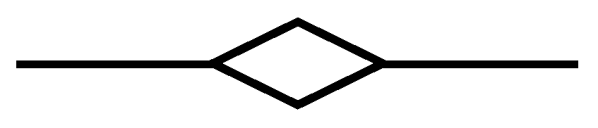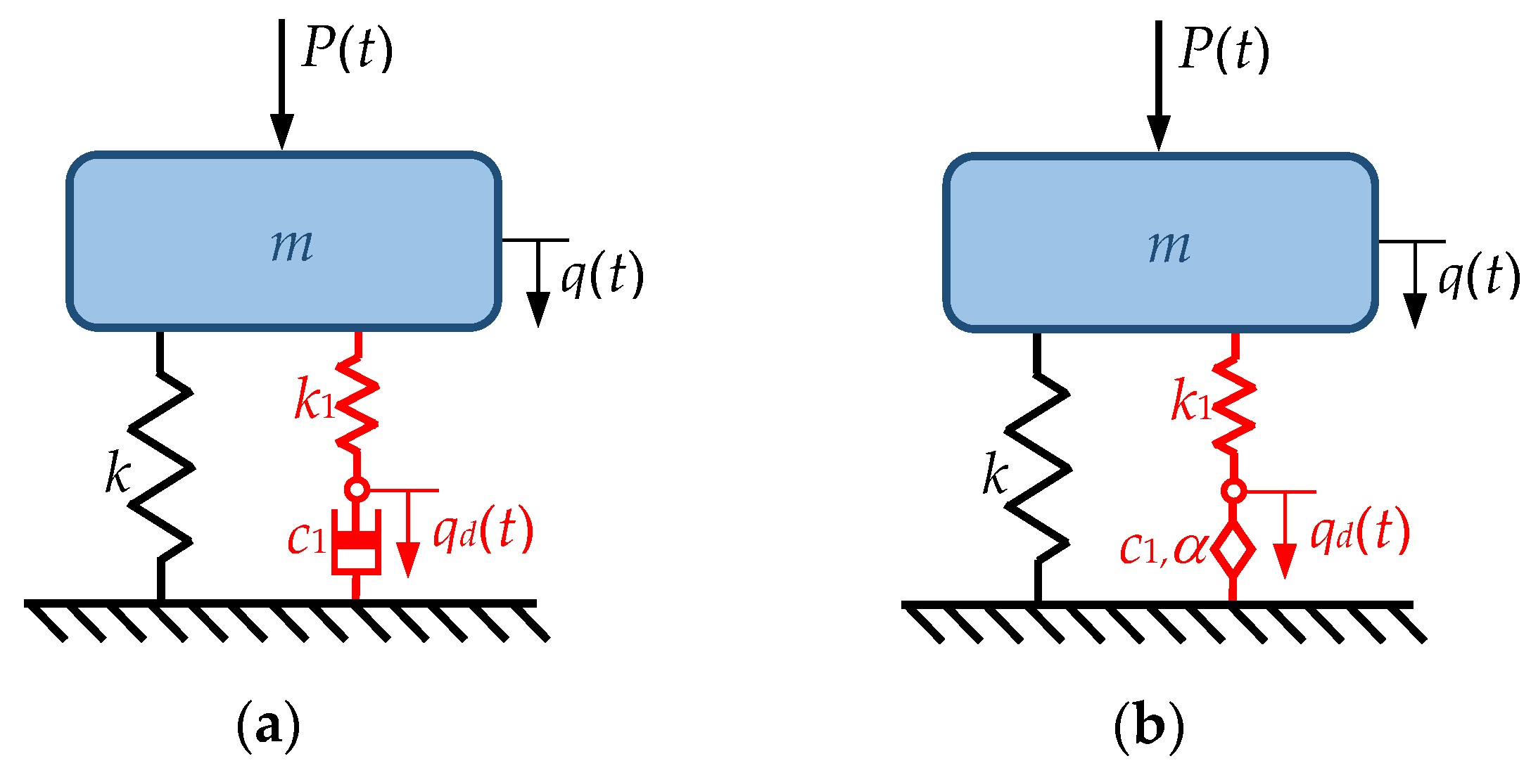In structural dynamics for matrix $\tilde{\mathbf{G}}\left(t-\tau \right)$, rheological models are commonly used, with fractional models being employed in this article. As part of this analysis, the Scott–Blair viscoelastic element (Figure 1) will be introduced. Its behavior is described by the following equation:

$$u\left(t\right)=c{D}_t^{\alpha }x\left(t\right)$$

(5)

where $c$ and $\alpha$ are the parameters of the described element $\left(0<\alpha \le 1\right)$, the symbol $D_t^{\alpha }\left(•\right)$ denotes the fractional derivative of order $\alpha$ with respect to time, and $x\left(t\right)$ is the difference in displacements of the damper nodes. $u\left(t\right)$ denotes the force in the viscoelastic element. A more extensive discussion of fractional calculus can be found in [48].

The following Riemann–Liouville definition of the fractional derivative was applied in the article:

$$D_t^{\alpha }x\left(t\right)=\frac{d^{\alpha }x\left(t\right)}{d{t}^{\alpha }}=\frac{1}{\mathsf{\Gamma }\left(1-\alpha \right)}\frac{d}{dt}\underset{0}{\overset{t}{\int }}\frac{x\left(s\right)}{{\left(t-s\right)}^{\alpha }}ds$$

(6)

where $\mathsf{\Gamma }$ denotes the gamma special function. As demonstrated in [49,50,51], the application of this definition is justified in the context of viscoelastic materials. In this article, Kelvin or Maxwell models will be considered, both classical and fractional (Figure 2). Classical models are described in [52] by Lewandowski et al., in [53] by Park, and in [54] by Hatada et al., and a description of fractional models can be found in [50] by Singh et al., in [51] by Lewandowski and Pawlak, and in [55] by Chang and Singh.

The force in the damping element, in the case of the Kelvin model, is described by the following equation:

$$u\left(t\right)=k_{0}x\left(t\right)+c_0{D}_t^{\alpha }x\left(t\right)$$

(7)

and for the Maxwell model, it is described as follows:

$$v_{1}u\left(t\right)+D_t^{\alpha }u\left(t\right)=k_1{D}_t^{\alpha }x\left(t\right)$$

(8)

where $c_0$ and $c_1$ are the damping coefficients of the Kelvin and Maxwell model, respectively, and $k_0$ and $k_1$ are the stiffness parameters of the Kelvin and Maxwell model, respectively. Additionally, $v_1=k_1/c_1$, and by achieving α = 1, one can obtain the classical models.

After applying the Laplace transformation, Equation (4) can be written as follows:

$$\left(s^2\mathbf{M}+s\mathbf{C}+\mathbf{K}+\mathbf{G}\left(s\right)\right)\tilde{\mathbf{q}}\left(s\right)=\tilde{\mathbf{P}}\left(s\right)$$

(9)

where $\tilde{\mathbf{q}}\left(s\right)$ and $\tilde{\mathbf{P}}\left(s\right)$ represent the Laplace transform of $\mathbf{q}\left(t\right)$ and $\mathbf{P}\left(t\right)$, respectively, and $\mathbf{G}\left(s\right)$ is the matrix of damping kernel functions in the Laplace domain. Its form depends on the adopted rheological model of the viscoelastic element, the considered structure, and the placement of the viscoelastic element. It can be expressed as the sum of matrices for individual viscoelastic elements, denoted as $\mathbf{G}\left(s\right)={\sum }_{k=1}^r{\mathbf{G}}_k\left(s\right)$ (where r denotes the number of viscoelastic elements).

Considering steady-state harmonic responses, the harmonic external forces can be described as follows:

$$\mathbf{P}\left(t\right)=\tilde{\mathbf{P}}\left(\lambda \right)\exp (\mathrm{i}\lambda t)$$

(10)

where $\tilde{\mathbf{P}}$ is the vector of excitation force amplitudes, and $\lambda$ is the frequency of excitation. The displacement of the structure can then be expressed as follows:

$$\mathbf{q}\left(\mathit{t}\right)=\tilde{\mathbf{q}}\left(\lambda \right)\mathbf{exp}(\mathrm{i}\lambda t)$$

(11)

Substituting (10) and (11) into Equation (4), we obtain the following formula:

$$\mathbf{D}\left(\lambda \right)\tilde{\mathbf{q}}\left(\lambda \right)=\tilde{\mathbf{P}}\left(\lambda \right)$$

(12)

where $\mathbf{D}\left(\lambda \right)$ is the dynamic stiffness matrix, which can also be obtained by substituting into Equation (9) $s=\mathrm{i}\lambda$.

$$\mathbf{D}\left(\lambda \right)=-{\lambda }^2\mathbf{M}+\mathrm{i}\lambda \mathbf{C}+\mathbf{K}+\sum _{k=1}^r{\mathbf{G}}_k\left(\lambda \right)$$

(13)

We assume that all design parameters can vary within certain specified bounds; therefore, we can represent them as interval numbers. The equation of motion in general form can be written as follows:

$$\left(-{\lambda }^2{\mathbf{M}}^I+\mathrm{i}\lambda {\mathbf{C}}^I+{\mathbf{K}}^I+\sum _{k=1}^r{\mathbf{G}}_k^I\left(\lambda \right)\right){\tilde{\mathbf{q}}}^I\left(\lambda \right)={\tilde{\mathbf{P}}}^I\left(\lambda \right)$$

(14)

or

$${\mathbf{D}}^I\left(\lambda \right){\tilde{\mathbf{q}}}^I\left(\lambda \right)={\tilde{\mathbf{P}}}^I\left(\lambda \right)$$

(15)

where

$${\mathbf{D}}^I\left(\lambda \right)=-{\lambda }^2{\mathbf{M}}^I+\mathrm{i}\lambda {\mathbf{C}}^I+{\mathbf{K}}^I+\sum _{k=1}^r{\mathbf{G}}_k^I\left(\lambda \right)$$

(16)

The solution to Equation (15) can be expressed as follows:

$${\tilde{\mathbf{q}}}^I\left(\lambda \right)={\mathbf{H}}^I\left(\lambda \right){\tilde{\mathbf{P}}}^I\left(\lambda \right)$$

(17)

where ${\mathbf{H}}^I\left(\lambda \right)$ denotes the interval frequency response function and can be determined as follows:

$${\mathbf{H}}^I\left(\lambda \right)={\left({\mathbf{D}}^I\left(\lambda \right)\right)}^{-1}={\left(-{\lambda }^2{\mathbf{M}}^I+\mathrm{i}\lambda {\mathbf{C}}^I+{\mathbf{K}}^I+\sum _{k=1}^r{\mathbf{G}}_k^I\left(\lambda \right)\right)}^{-1}$$

(18)

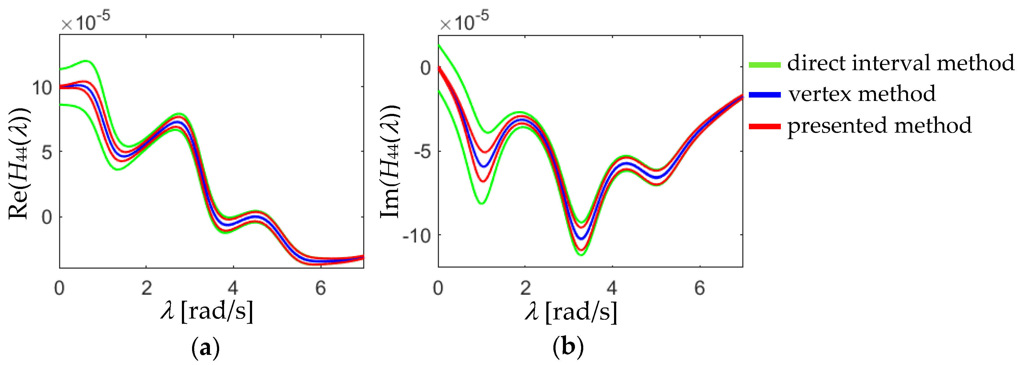
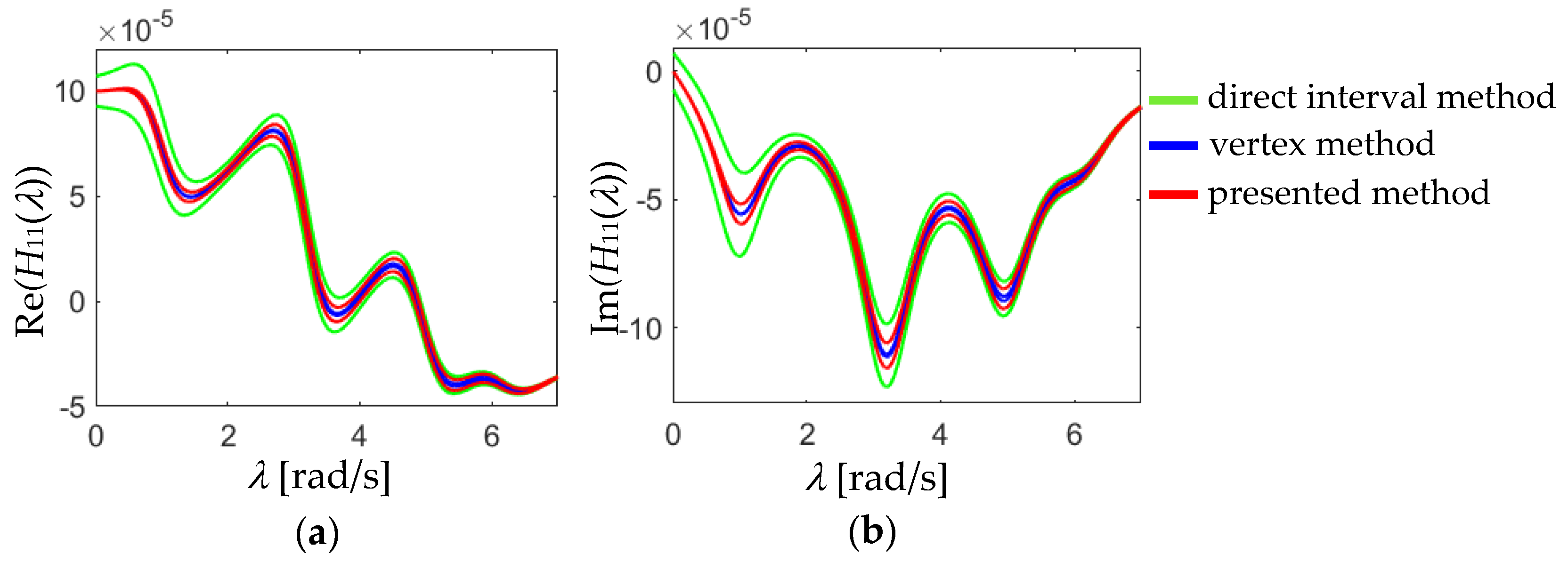
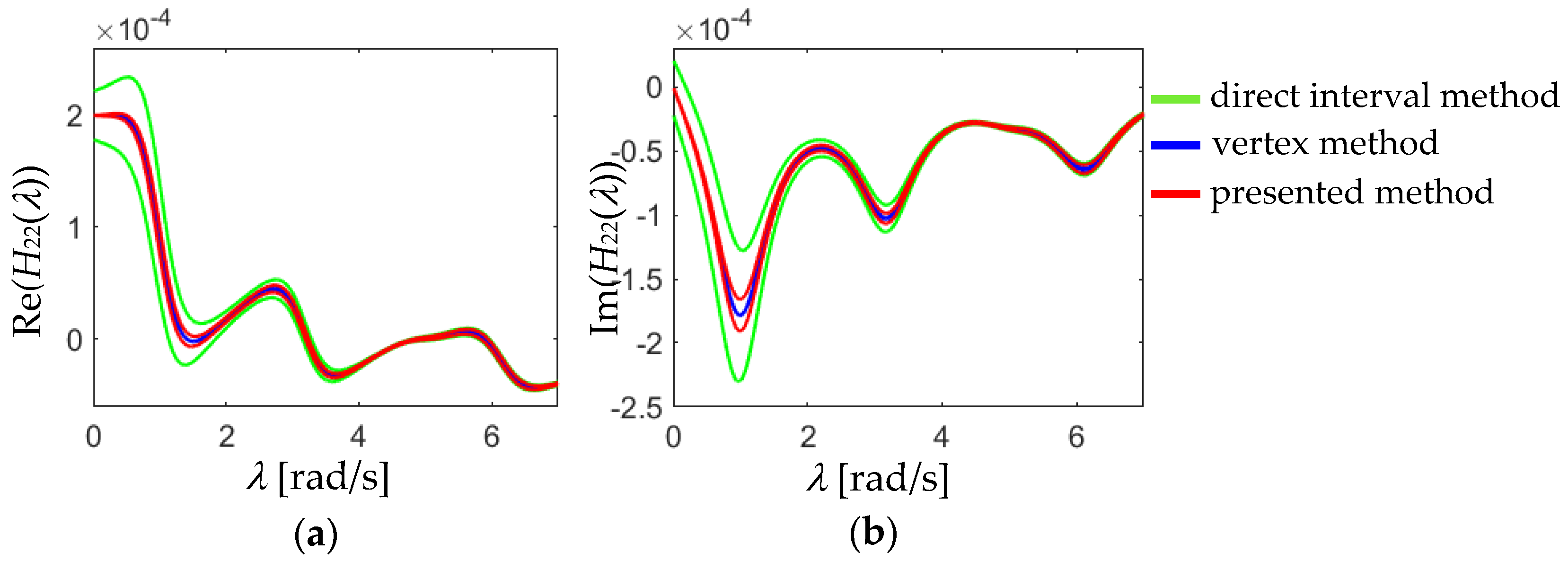
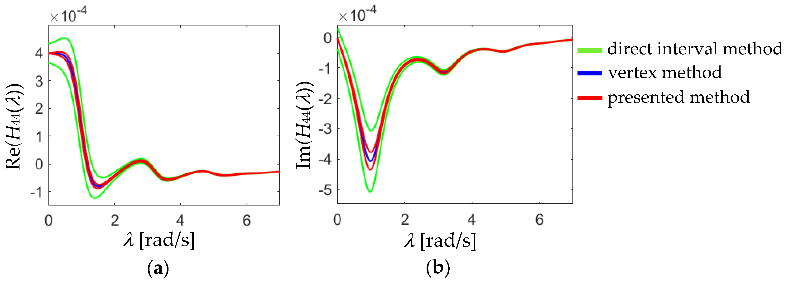
The individual elements of the matrix ${\mathbf{H}}^I\left(\lambda \right)$ with indices i and j can be interpreted as the frequency response function determined for the degree of freedom with index i when unit harmonic excitation acts in the direction of the dynamic degree of freedom of the structure with index j. Determining the FRF matrix from Equation (18) requires the direct application of interval arithmetic. This method will later be referred to as the direct interval method (DIM). However, as demonstrated in the examples presented, this approach leads to significant overestimations, as described by Yaowen et al. in [44] and Moens and Vandepitte in [13].

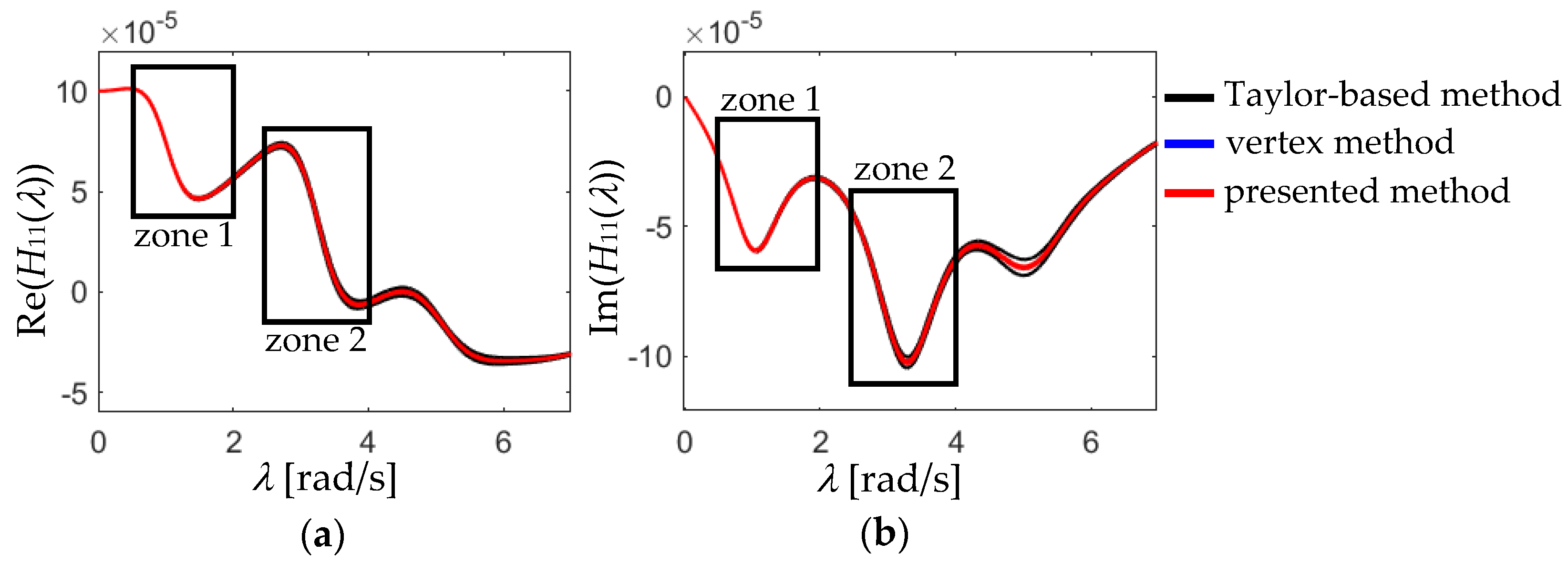
To mitigate the overestimation, a method will be applied where the calculation of the FRF matrix will be divided into steps, computing each column of the matrix ${\mathbf{H}}^I\left(\lambda \right)$ sequentially. Since the dynamic response of the structure, understood as vector ${\tilde{\mathbf{q}}}^I\left(\lambda \right)$, can be obtained using Equation (17), it is worth noting that if we represent the vector ${\tilde{\mathbf{P}}}^I\left(\lambda \right)$ as

$$\mathbf{P}={\left[\begin{array}{cccc}1& 0& \dots & 0\end{array}\right]}^T$$

(19)

the first column of the matrix ${\mathbf{H}}^I\left(\lambda \right)$ will be determined. Subsequent columns can be obtained by substituting value 1 at successive positions in vector $\mathbf{P}$. This approach involves solving interval equation systems to compute the FRF matrix. Various iterative methods that can be applied for this purpose are presented by Rump in [47,56] and Jansson in [57]. The specific method used in this work will be described in the next section.

4. Interval Equations System Solving

In the paper, Brower’s fixed-point theorem was applied to solve the system of linear interval equations (Rump [47], Neumaier [58]):

$${\mathbf{D}}^I\left(\lambda \right){\tilde{\mathbf{q}}}^I\left(\lambda \right)={\tilde{\mathbf{P}}}^I\left(\lambda \right)$$

(20)

after substituting the appropriate vector ${\tilde{\mathbf{P}}}^I\left(\lambda \right)$.

Equation (20) can be transformed into a fixed-point equation in the following form:

$$g\left({\tilde{\mathbf{q}}}^I\right)={\tilde{\mathbf{q}}}^I$$

(21)

where

$$g\left({\tilde{\mathbf{q}}}^I\right)={\tilde{\mathbf{q}}}^I-\mathbf{R}\left({\mathbf{D}}^I{\tilde{\mathbf{q}}}^I-{\tilde{\mathbf{P}}}^I\right)=\mathbf{R}{\tilde{\mathbf{P}}}^I+\left(\mathbf{I}-\mathbf{R}{\mathbf{D}}^I\right){\tilde{\mathbf{q}}}^I$$

(22)

and $\mathbf{R}$ is a nonsingular matrix. In Equation (22), all quantities except $\mathbf{R}$ are interval numbers.

Using Brower’s fixed-point theorem, we can express the following:

$$\mathbf{R}{\tilde{\mathbf{P}}}^I+\left(\mathbf{I}-\mathbf{R}{\mathbf{D}}^I\right){\tilde{\mathbf{q}}}^I\in {\tilde{\mathbf{q}}}^I$$

(23)

The solution to Equation (23) also satisfies the original Equation (20). Therefore, it is possible to write the following (Rump [59]):

$$\mathbf{R}{\tilde{\mathbf{P}}}^I+\left(\mathbf{I}-\mathbf{R}{\mathbf{D}}^I\right){\tilde{\mathbf{q}}}^I\subseteq \mathit{int}\left({\tilde{\mathbf{q}}}^I\right)$$

(24)

where $\mathit{int}\left({\tilde{\mathbf{q}}}^I\right)$ denotes interior of ${\tilde{\mathbf{q}}}^I$.

If we denote that ${\tilde{\mathbf{q}}}^I={\tilde{\mathbf{q}}}^C+{\widehat{\mathbf{q}}}^I$, where ${\tilde{\mathbf{q}}}^C$ is the computed vector for the central values of the parameters, and ${\widehat{\mathbf{q}}}^I$ is the uncertainty of the solution, then Equation (24) can be expressed as follows (Neumaier [45]):

$$\mathbf{R}{\tilde{\mathbf{P}}}^I-\mathbf{R}{\mathbf{D}}^I{\tilde{\mathbf{q}}}^C+\left(\mathbf{I}-\mathbf{R}{\mathbf{D}}^I\right){\widehat{\mathbf{q}}}^I\subseteq \mathit{int}\left({\widehat{\mathbf{q}}}^I\right)$$

(25)

The equation used for the iterative determination of the uncertainty of the solution can thus be written as follows:

$${\left({\widehat{\mathbf{q}}}^I\right)}^{n+1}=\mathbf{R}{\tilde{\mathbf{P}}}^I-\mathbf{R}{\mathbf{D}}^I{\tilde{\mathbf{q}}}^C+\left(\mathbf{I}-\mathbf{R}{\mathbf{D}}^I\right){\left({\widehat{\mathbf{q}}}^I\right)}^n$$

(26)

According to work [45] by Neumaier, the matrix $\mathbf{R}$ is defined as $\mathbf{R}={\left({\mathbf{D}}^C\right)}^{-1}={\mathbf{H}}^C$. The stopping criterion for the iteration is as follows:

$${\left({\widehat{\mathbf{q}}}^I\right)}^{n+1}\subseteq {\left({\widehat{\mathbf{q}}}^I\right)}^n$$

(27)

The final value of the solution is obtained based on the following equation:

$${\tilde{\mathbf{q}}}^I={\left({\widehat{\mathbf{q}}}^I\right)}^{n+1}+{\tilde{\mathbf{q}}}^C$$

(28)

The above algorithm can be successfully applied to solve systems of linear interval equations, as demonstrated in [43] by Muhanna and Zhang.

5. Application of the Presented Method to Multi-Degrees-of-Freedom Systems with Viscoelastic Elements

The matrix-form equation of motion for systems with viscoelastic elements is given in the form (12). However, such representation leads to interval quantities associated with one physical quantity appearing more than once, which can cause significant overestimations. As demonstrated Muhanna and Zhang in [43] for statics and Yaowen et al. in [44] for dynamics, overestimation is reduced by applying the element-by-element technique. This approach is detailed in [44] by Yaowen et al. As a result of employing this technique, we obtain a singular stiffness matrix. Hence, it is necessary to introduce an additional constraint matrix $\mathbf{X}$ for the considered system and apply the Lagrange multiplier method ${(\mathsf{\beta }}^I)$. Then, the equation of motion looks as follows:

$$\left[\begin{array}{cc}{\mathbf{K}}^I+\mathrm{i}\lambda {\mathbf{C}}^I-{\lambda }^2{\mathbf{M}}^I+{\mathbf{G}}^I\left(\lambda \right)& {\mathbf{X}}^T\\ \mathbf{X}& 0\end{array}\right]\left[\begin{array}{c}\tilde{\mathbf{q}}{\left(\lambda \right)}^I\\ {\mathsf{\beta }}^I\end{array}\right]=\left[\begin{array}{c}\tilde{\mathbf{P}}{\left(\lambda \right)}^I\\ 0\end{array}\right]$$

(29)

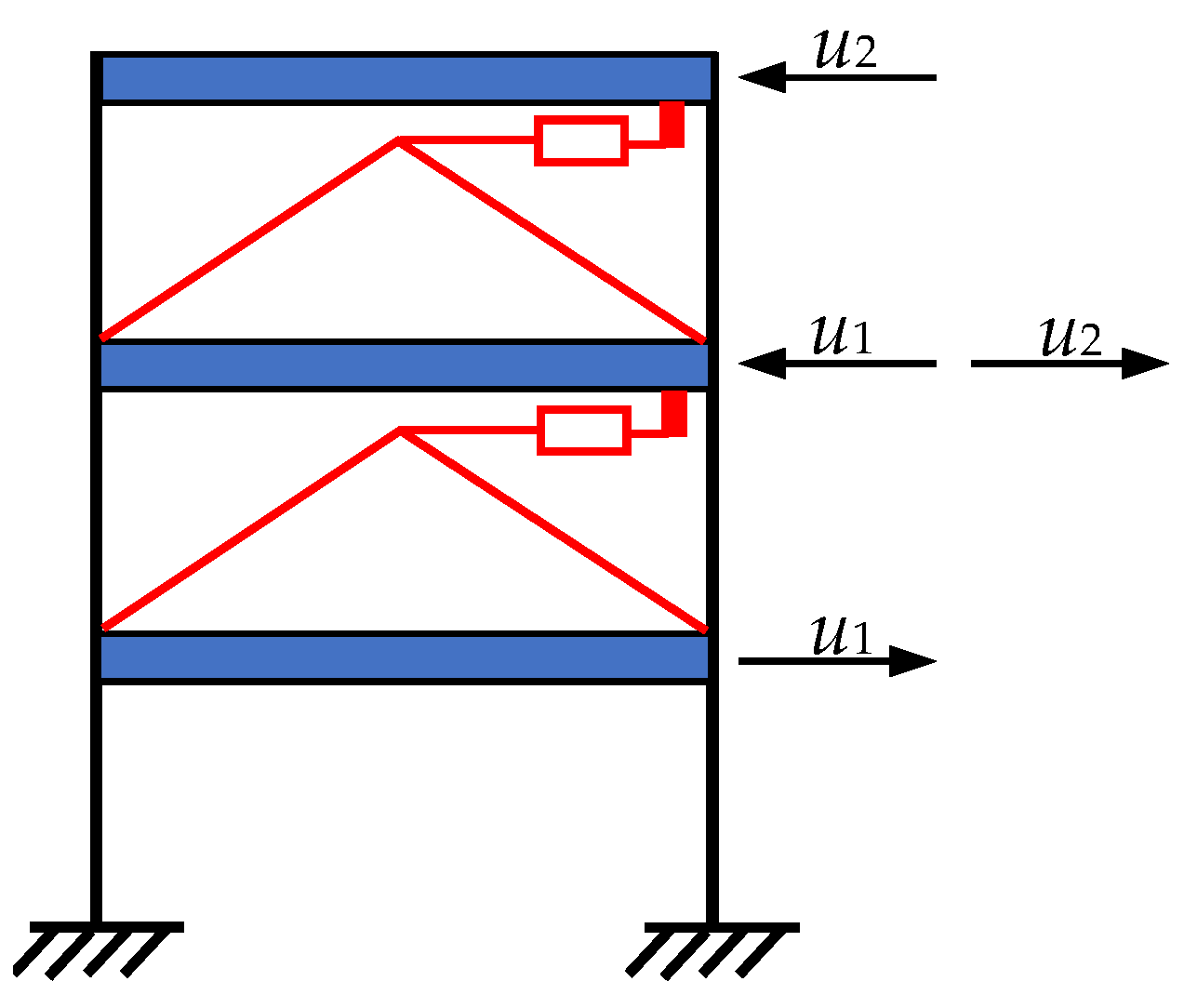
where interval vectors and matrices are constructed using the element-by-element technique. This technique will be demonstrated based on the construction of the component matrix ${\mathbf{G}}^I\left(\lambda \right)$. Let us consider a three-story frame, as shown in Figure 3, with two dampers described by the Kelvin model. The schematic illustrates the forces $u_i$, representing the interactions of individual dampers with each floor.

The matrix containing uncertain damping parameters $c_{0k}^I$ will be considered. According to [51] by Lewandowski and Pawlak and [52] by Lewandowski et al., for one damper k, the matrix can be expressed as follows:

$${\mathbf{C}}_{0k}^I=\left[\begin{array}{cc}{c}_{0k}^I& -c_{0k}^I\\ -c_{0k}^I& c_{0k}^I\end{array}\right]=\left[\begin{array}{cc}{c}_{0k}^C& -c_{0k}^C\\ -c_{0k}^C& c_{0k}^C\end{array}\right]\left(\left[\begin{array}{cc}1& 0\\ 0& 1\end{array}\right]+\left[\begin{array}{cc}{\delta }_k^I& 0\\ 0& {\delta }_k^I\end{array}\right]\right)={\mathbf{C}}_{0k}^C\left(\mathbf{I}+{\mathsf{\delta }}_k^I\right)$$

(30)

where $c_{0k}^I$ is the uncertain damping parameter of damper k, $c_{0k}^C$ is the central value of parameter $c_{0k}^I$, and ${\delta }_k^I$ denotes the uncertainty of parameter $c_{0k}^I$.

If we consider two dampers, it is possible to express the matrix ${\mathbf{C}}_0^I$ in the following form:

$$\begin{gathered} {\mathbf{C}}_0^I=\left[\begin{array}{cccc}{c}_{01}^I& -c_{01}^I& 0& 0\\ -c_{01}^I& c_{01}^I& 0& 0\\ 0& 0& c_{02}^I& -c_{02}^I\\ 0& 0& -c_{02}^I& c_{02}^I\end{array}\right]= \\ =\left[\begin{array}{cccc}{c}_{01}^C& -c_{01}^C& 0& 0\\ -c_{01}^C& c_{01}^C& 0& 0\\ 0& 0& c_{02}^C& -c_{02}^C\\ 0& 0& -c_{02}^C& c_{02}^C\end{array}\right]\left(\left[\begin{array}{cccc}1& 0& 0& 0\\ 0& 1& 0& 0\\ 0& 0& 1& 0\\ 0& 0& 0& 1\end{array}\right]+\left[\begin{array}{cccc}{\delta }_1^I& 0& 0& 0\\ 0& {\delta }_1^I& 0& 0\\ 0& 0& {\delta }_2^I& 0\\ 0& 0& 0& {\delta }_2^I\end{array}\right]\right)={\mathbf{C}}_0^C\left(\mathbf{I}+{\mathsf{\Delta }}^I\right) \end{gathered}$$

(31)

It is worth noting that Formula (31) aims to illustrate only the idea of the element-by-element technique using the example of coefficients for two dampers, and it is not the final form of the matrix appearing in the equation of motion. From the above expression, it is clear that one uncertain parameter associated with the damper appears four times, meaning the uncertainties ${\delta }_k^I$ overlap and cause overestimation.

According to the above notation, the remaining matrices can be expressed as follows:

$${\mathbf{K}}^I={\mathbf{K}}^C\left(\mathbf{I}+{\mathsf{\Delta }}_1^I\right), {\mathbf{C}}^I={\mathbf{C}}^C\left(\mathbf{I}+{\mathsf{\Delta }}_2^I\right), {\mathbf{M}}^I={\mathbf{M}}^C\left(\mathbf{I}+{\mathsf{\Delta }}_3^I\right), {\mathbf{G}}^I\left(\lambda \right)={\mathbf{G}}^C\left(\lambda \right)\left(\mathbf{I}+{\mathsf{\Delta }}_4^I\right)$$

(32)

and the equation of motion takes the following form:

$$\begin{gathered} \left[\left[\begin{array}{cc}{\mathbf{K}}^C+\mathrm{i}\lambda {\mathbf{C}}^C-{\lambda }^2{\mathbf{M}}^C+{\mathbf{G}}^C\left(\lambda \right)& {\mathbf{X}}^T\\ \mathbf{X}& \mathbf{0}\end{array}\right]\right.+\left[\begin{array}{cc}{\mathbf{K}}^C& \mathbf{0}\\ \mathbf{0}& \mathbf{0}\end{array}\right]\left[\begin{array}{cc}{\mathsf{\Delta }}_1^I& \mathbf{0}\\ \mathbf{0}& \mathbf{0}\end{array}\right] \\ +\mathrm{i}\lambda \left[\begin{array}{cc}{\mathbf{C}}^C& \mathbf{0}\\ \mathbf{0}& \mathbf{0}\end{array}\right]\left[\begin{array}{cc}{\mathsf{\Delta }}_2^I& \mathbf{0}\\ \mathbf{0}& \mathbf{0}\end{array}\right]\left.-{\lambda }^2\left[\begin{array}{cc}{\mathbf{M}}^C& \mathbf{0}\\ \mathbf{0}& \mathbf{0}\end{array}\right]\left[\begin{array}{cc}{\mathsf{\Delta }}_3^I& \mathbf{0}\\ \mathbf{0}& \mathbf{0}\end{array}\right]+\left[\begin{array}{cc}{\mathbf{G}}^C\left(\lambda \right)& \mathbf{0}\\ \mathbf{0}& \mathbf{0}\end{array}\right]\left[\begin{array}{cc}{\mathsf{\Delta }}_4^I& \mathbf{0}\\ \mathbf{0}& \mathbf{0}\end{array}\right]\right]\left[\begin{array}{c}{\tilde{\mathbf{q}}}^I\\ {\mathsf{\beta }}^I\end{array}\right]=\left[\begin{array}{c}{\tilde{\mathbf{P}}}^I\\ \mathbf{0}\end{array}\right] \end{gathered}$$

(33)

To reduce overestimation when multiplying any matrix by a displacement vector, the following transformation will be applied, expressed in the general form for quantities ${\mathsf{\Delta }}_k^I$ and ${\tilde{\mathbf{q}}}^I$:

$$\left[\begin{array}{ccccccc}{\delta }_1^I& 0& 0& 0& \dots & 0& 0\\ 0& {\delta }_1^I& 0& 0& \dots & 0& 0\\ 0& 0& {\delta }_2^I& 0& \dots & 0& 0\\ 0& 0& 0& {\delta }_2^I& \dots & 0& 0\\ \dots & \dots & \dots & \dots & \dots & \dots & \dots \\ 0& 0& 0& 0& \dots & {\delta }_n^I& 0\\ 0& 0& 0& 0& \dots & 0& {\delta }_n^I\end{array}\right]\left[\begin{array}{c}{q}_1^I\\ q_2^I\\ q_3^I\\ q_4^I\\ \dots \\ q_{2n-1}^I\\ q_{2n}^I\end{array}\right]=\left[\begin{array}{cccc}{q}_1^I& 0& \dots & 0\\ q_2^I& 0& \dots & 0\\ 0& q_3^I& \dots & 0\\ 0& q_4^I& \dots & 0\\ \dots & \dots & \dots & \dots \\ 0& 0& \dots & q_{2n-1}^I\\ 0& 0& \dots & q_{2n}^I\end{array}\right]\left[\begin{array}{c}{\delta }_1^I\\ {\delta }_2^I\\ \dots \\ {\delta }_n^I\end{array}\right]={\mathbf{Q}}^I{\mathbf{d}}^I$$

(34)

The above transformation ensures that each uncertain parameter associated with quantity i appears only once. Equation (33) can be rewritten in the following form:

$$\left({\overline{\mathbf{D}}}^C+{\overline{\mathbf{K}}}^C{\overline{\mathsf{\Delta }}}_1^I+i\mathrm{i}\lambda {\overline{\mathbf{C}}}^C{\overline{\mathsf{\Delta }}}_2^I-{\lambda }^2{\overline{\mathbf{M}}}^C{\overline{\mathsf{\Delta }}}_3^I+{\overline{\mathbf{G}}}^C\left(\lambda \right){\overline{\mathsf{\Delta }}}_2^I\right){\overline{\mathbf{Q}}}^I={\overline{\mathbf{P}}}^I$$

(35)

or in a more compact form, as follows:

$$\left({\overline{\mathbf{D}}}^C+{\overline{\mathbf{D}}}_1^I\right){\overline{\mathbf{Q}}}^I={\overline{\mathbf{P}}}^I$$

(36)

where ${\overline{\mathbf{D}}}_1^I={\sum }_{i=1}^4{\mathsf{\Psi }}_i{\overline{\mathsf{\Delta }}}_i^I$, ${\mathsf{\Psi }}_1={\overline{\mathbf{K}}}^C$, ${\mathsf{\Psi }}_2=\mathrm{i}\lambda {\overline{\mathbf{C}}}^C$, ${\mathsf{\Psi }}_3=-{\lambda }^2{\overline{\mathbf{M}}}^C$ and ${\mathsf{\Psi }}_4={\overline{\mathbf{G}}}^C\left(\lambda \right)$.

Assuming that Equation (36) can be treated as a system of linear interval equations, Equation (26) can be written in the following form:

$${\left({\widehat{\mathbf{Q}}}^I\right)}^{n+1}=\mathbf{R}{\overline{\mathbf{P}}}^I-\mathbf{R}{\overline{\mathbf{D}}}^I{\mathbf{Q}}^C+\left(\mathbf{I}-\mathbf{R}{\overline{\mathbf{D}}}^I\right){\left({\widehat{\mathbf{Q}}}^I\right)}^n$$

(37)

and after considering (36) and $\mathbf{R}={\left({\overline{\mathbf{D}}}^C\right)}^{-1}$, we obtain the iterative equation in the following form:

$${\left({\widehat{\mathbf{Q}}}^I\right)}^{n+1}=\mathbf{R}{\overline{\mathbf{P}}}^I-{\mathbf{Q}}^C-\mathbf{R}{\overline{\mathbf{D}}}_1^I\left({\mathbf{Q}}^C+{\left({\widehat{\mathbf{Q}}}^I\right)}^n\right)$$

(38)

In Equation (38), in the case of multiplication ${\overline{\mathbf{D}}}_1^I{\left({\widehat{\mathbf{Q}}}^I\right)}^n$, we apply transformation (34).

6. Examples

6.1. Single-DOF System: Kelvin Model of Viscoelastic Element

To illustrate the method’s idea, we will first discuss the single-degree-of-freedom system with a Kelvin damper, both fractional and classical, as shown in Figure 4. The equation of motion (15), assuming that the system parameters are described using interval numbers, now takes the following form:

$$-{\lambda }^2{m}^I{\tilde{q}}^I\left(\lambda \right)+k_s^I{\tilde{q}}^I\left(\lambda \right)+k_0^I{\tilde{q}}^I\left(\lambda \right)+{\left(\mathrm{i}\lambda \right)}^{\alpha }{c}_0^I{\tilde{q}}^I\left(\lambda \right)={\tilde{P}}^I\left(\lambda \right)$$

(39)

where $m$ and $k$ are understood as the mass and stiffness of the system, respectively, and $k_0$, $c_0$, and $\alpha$ represent the stiffness, damping coefficient, and the order of the fractional derivative describing the parameters of the Kelvin damper, respectively. ${\tilde{P}}^I\left(\lambda \right)$ denotes the forcing function, and ${\tilde{q}}^I\left(\lambda \right)$ represents the displacement of the considered system. The task is to find the system response in the form of displacement values.

We assumed the following parameters for the analyzed system: $m=40 \mathrm{k}\mathrm{g}$, $k_s=1000 \mathrm{N}/\mathrm{m}$, $k_0=500 \mathrm{N}/\mathrm{m}$. Various cases of damping coefficients were analyzed, with the data shown in

Table 1. Values of parameters for example 6.1.

Case	$\mathbf{Damping} \mathbf{Coefficient} {\mathit{c}}_0$ [Nsα/m]	Fractional Order α	Natural Frequency ω [rad/s]	Nondimensional Damping Ratio γ [-]
1	80	1.0	6.1237	0.1633
2	120	1.0	6.1237	0.2449
3	80	0.8	6.3567	0.1064
4	120	0.8	6.4884	0.1583

. It was assumed that the forcing magnitude $P_0=1 \mathrm{N}$ and is not affected by uncertainties. Only the stiffness and damping parameters of the viscoelastic element are uncertain, with 5% uncertainty.

Table 2. Ranges of parameters for the damper for example 6.1.

Case	$\mathbf{Damping} \mathbf{Coefficient} {\mathit{c}}_0^{\mathit{I}}$ [Nsα/m]	$\mathbf{Stiffness} \mathbf{Coefficient} {\mathit{k}}_0^{\mathit{I}}$ [Ns/m]
1	[76, 84]	[475, 525]
2	[114, 126]	[475, 525]
3	[76, 84]	[475, 525]
4	[114, 126]	[475, 525]

presents the parameter values in the form of interval numbers. The response of the structure was calculated using the vertex method (red line), DIM (green line), and the method described in the article (blue line). The results are presented in Figure 5, Figure 6, Figure 7 and Figure 8. The zoomed-in figures show only the region near the resonance zone because in other areas, the results are practically overlapping.

In the first two cases, the classical Kelvin model was considered (Figure 5 and Figure 6), while in the next two, the fractional model was analyzed (Figure 7 and Figure 8).

The results for the presented method and for the DIM almost overlap, especially when the system’s damping is higher. The obtained results are also very close to those of the vertex method, indicating that the presented method can assess the influence of uncertain design parameters on the system’s response. In all cases, the results of the presented method lie outside the interval obtained from the vertex method, indicating that they are on the safe side. The example shown demonstrates that the presented method can be applied to determine the response of a system with a viscoelastic element described using both classical and fractional Kelvin models.

6.2. Single-DOF System—Maxwell Model of Viscoelastic Element

The system under consideration is a single-degree-of-freedom system, as depicted in Figure 9, where the viscoelastic element is described using the Maxwell model. The presented method requires the equations of motion to be formulated in a way that describes the relationship between the central value of the parameter and its uncertainties, as outlined in Equation (31). In the case of the Kelvin model, as discussed in the previous section, achieving this is relatively straightforward. However, for the Maxwell model, it is necessary to use a representation involving an internal variable indicated in Figure 9 as $q_d$ (Lewandowski et al. [52]). The equations of motion then take on the following form:

$$\begin{gathered} -{\lambda }^2{m}^I{\tilde{q}}^I\left(\lambda \right)+k_s^I{\tilde{q}}^I\left(\lambda \right)+{\left(\mathrm{i}\lambda \right)}^{\alpha }{c}_1^I{\tilde{q}}^I\left(\lambda \right)-{\left(\mathrm{i}\lambda \right)}^{\alpha }{c}_1^I{\tilde{q}}_d^I\left(\lambda \right) \\ ={\tilde{P}}^I\left(\lambda \right)-{\left(\mathrm{i}\lambda \right)}^{\alpha }{c}_1^I{\tilde{q}}^I\left(\lambda \right)+{\left(\mathrm{i}\lambda \right)}^{\alpha }{c}_1^I{\tilde{q}}_d^I\left(\lambda \right)+k_1^I{\tilde{q}}_d^I\left(\lambda \right)=0 \end{gathered}$$

(40)

or the following matrix form:

$$-{\lambda }^2\left[\begin{array}{cc}{m}^I& 0\\ 0& 0\end{array}\right]\left[\begin{array}{c}{\tilde{q}}^I\left(\lambda \right)\\ {\tilde{q}}_d^I\left(\lambda \right)\end{array}\right]+{\left(\mathrm{i}\lambda \right)}^{\alpha }{c}_1^I\left[\begin{array}{cc}1& -1\\ -1& 1\end{array}\right]\left[\begin{array}{c}{\tilde{q}}^I\left(\lambda \right)\\ {\tilde{q}}_d^I\left(\lambda \right)\end{array}\right]+\left[\begin{array}{cc}{k}_s^I& 0\\ 0& k_1^I\end{array}\right]\left[\begin{array}{c}{\tilde{q}}^I\left(\lambda \right)\\ {\tilde{q}}_d^I\left(\lambda \right)\end{array}\right]=\left[\begin{array}{c}{\tilde{P}}^I\left(\lambda \right)\\ 0\end{array}\right]$$

(41)

From this expression, it is evident that even in a simple case like a single-degree-of-freedom system, when dealing with the damping parameter of the Maxwell model, there might be overestimation. This results from the fact that the interval number describing one parameter appears four times in the expression (refer to the second term of Equation (41)). To investigate the potential for reducing overestimation with the applied method, two cases were examined in the computed examples. In the first case, the transformation described by Equations (34) was not applied (Figure 10 and Figure 11, while in the second case, the transformations (34) were applied (Figure 12 and Figure 13). The analyzed system is characterized by the following parameters: $m=40 \mathrm{k}\mathrm{g}$, $k_s=1000 \mathrm{N}/\mathrm{m}$, and $k_1=500 \mathrm{N}/\mathrm{m}$. Two different damping parameter values were assumed, as detailed in

Table 3. Values of parameters for example 6.2.

Case	$\mathbf{Damping} \mathbf{Coefficient} {\mathit{c}}_1$ [Nsα/m]	Fractional Order α	Natural Frequency ω [rad/s]	Nondimensional Damping Ratio γ [-]
1	120	1.0	5.8398	0.0952
2	80	0.8	5.4130	0.0756

. Similar to example 6.1, the parameters of the viscoelastic damper have 5% uncertainty. The parameter values are listed in

Table 4. Ranges of parameters for the damper for example 6.2.

Case	$\mathbf{Damping} \mathbf{Coefficient} {\mathit{c}}_1^{\mathit{I}}$ [Nsα/m]	$\mathbf{Stiffness} \mathbf{Coefficient} {\mathit{k}}_1^{\mathit{I}}$ [Ns/m]
1	[114, 126]	[475, 525]
2	[76, 84]	[475, 525]

.

The results are calculated using three methods: vertex, DIM, and the presented method.

In the cases considered without ransformation (34), the results from the presented method and the DIM are almost identical, leading to overlapping plots in most instances. However, it is important to note that there is an overestimation, particularly evident in the example shown in Figure 10. In this case, the plots do not resemble the results from the vertex method at all, indicating complete inaccuracy. On the other hand, applying transformation (34) brings the results obtained using the fixed-point iteration method closer to those from the vertex method, leading to a significant reduction in overestimation.

Both in examples 6.1 and 6.2, the results are magnified for the resonance zone, as the outcomes in this zone are significant from an engineering perspective. The differences visible in the plots are thus emphasized through magnification. Based on the presented examples, it is also noticeable that the presented method provides more accurate results when the nondimensional damping ratio of the analyzed system is higher.

6.3. Frame with Kelvin Models

The structure under consideration is a frame with dampers described by the fractional Kelvin model, as shown in Figure 14. The parameters of the frame are as follows: the mass of the floor is $m=1000 \mathrm{k}\mathrm{g}$, and the stiffness of the storey is $k=\mathrm{10,000} \mathrm{N}/\mathrm{m}$. Structural damping is assumed to be proportional and described by the relationship $\mathbf{C}=0.001 \mathbf{K}+1.0 \mathbf{M}$. Additionally, all dampers are assumed to be the same and described by the following parameters: $k_0=1000 \mathrm{N}/\mathrm{m}$, $c_0=500 \mathrm{N}{\mathrm{s}}^{\mathsf{\alpha }}/\mathrm{m}$, and $\alpha =0.8$. The natural frequencies and the nondimensional damping ratios for the analyzed frame are presented in

Table 5. Dynamic characteristics of the frame from example 6.3.

Mode	Natural Frequency ω [rad/s]	Nondimensional Damping Ratio γ [-]
1	1.1349	0.4562
2	3.3113	0.1909
3	5.1591	0.1664
4	6.4217	0.1710

. The parameters of the dampers $c_0$ and $k_0$ are uncertain, with 5% uncertainty assumed for each parameter independently. The parameters of the dampers can be described as follows:

$$c_{0i}^I=c_{0i}^C\left(1+{\delta }_i^I\right),{ k}_{0i}^I=k_{0i}^C\left(1+{\delta }_i^I\right)$$

(42)

where ${\delta }_i^I=\left[-0.05, 0.05\right]$. The matrix ${\overline{\mathbf{D}}}_1^I$ appearing in Equation (36) has the following form:

$${\overline{\mathbf{D}}}_1^I={\left(\mathrm{i}\lambda \right)}^{\alpha }{\overline{\mathbf{C}}}_0^C{\overline{\mathsf{\Delta }}}_1^I+{\overline{\mathbf{K}}}_0^C{\overline{\mathsf{\Delta }}}_2^I$$

(43)

where the matrices ${\overline{\mathbf{C}}}_0^C$ and ${\overline{\mathbf{K}}}_0^C$ contain the central values of the damping coefficients and stiffness coefficients of the dampers, respectively, while ${\overline{\mathsf{\Delta }}}_1^I$ and ${\overline{\mathsf{\Delta }}}_2^I$ contain the uncertainties of these parameters. All matrices in Equation (43) are constructed using the element-by-element technique, and transformation (34) has been applied in the calculations. The real and imaginary parts of selected elements of the FRF matrix are shown in Figure 15, Figure 16, Figure 17 and Figure 18.

Based on Figure 15, Figure 16, Figure 17 and Figure 18, it is evident that the presented method yields results close to the vertex method. Moreover, compared to the DIM, it significantly reduces overestimation resulting from the direct analysis in interval arithmetic, especially at lower frequencies. This confirms the advantages of the presented method. Additionally, considering the computational cost of the presented method and the vertex method, the presented method also holds an advantage. In the case of the vertex method and six varying parameters, the number of cases to be considered for each analyzed frequency is $2^6=64$, whereas with the presented method, the solution is typically obtained after a few iterations and is relatively straightforward to implement.

In

Table 6. Errors for uncertainties of 5%.

$\mathbf{Frequency} \mathit{\lambda }$ [rad/s]	Error of Direct Interval Method [%]		Error of Presented Method [%]
	Upper Bound	Lower Bound	Upper Bound	Lower Bound
0.5	8.73	7.03	0.63	0.62
1.1	3.88	1.74	0.66	0.13
2.0	1.87	1.41	0.71	0.60
3.2	2.69	3.41	1.41	1.62
5.2	3.64	3.51	2.94	2.82
6.4	1.75	1.67	1.66	1.59
7.0	1.02	0.98	1.01	0.98

and

Table 7. Errors for uncertainties of 1%.

$\mathbf{Frequency} \mathit{\lambda }$ [rad/s]	Error of Direct Interval Method [%]		Error of Presented Method [%]
	Upper Bound	Lower Bound	Upper Bound	Lower Bound
0.5	1.40	1.35	0.07	0.07
1.1	0.26	0.11	0.05	0.04
2.0	0.31	0.29	0.09	0.09
3.2	0.56	0.58	0.22	0.22
5.2	0.67	0.66	0.44	0.44
6.4	0.32	0.32	0.26	0.25
7.0	0.19	0.19	0.17	0.17

, the relative error for the presented method and the direct method is shown for selected values of frequency and two uncertainty values: 5% and 1%. The absolute errors of the magnitude for $H_{11}$ were calculated. The vertex method was adopted as a comparative method.

Based on the results presented in Table 6 and Table 7, it can be observed that the error values are always smaller in the case of the presented method. The largest differences are for lower frequencies, which confirms the observations from the $H_{11}$ plots, where the largest overestimations for the direct method are indeed in this area. The obtained results confirm the superiority of the presented approach over the direct interval method.

In

Table 8. Solution times.

Uncertainties of Parameters [%]	Presented Method [s]	Vertex Method [s]
5	4.400	7.497
4	3.791	7.457
3	3.252	7.382
2	2.756	7.456
1	2.236	7.512
0.5	1.896	7.380

, the computation time for H₁₁ is presented for various uncertainty values. Based on the example provided, it can be observed that the discussed iterative method is more efficient, the smaller the uncertainties are. This is associated with a lower number of iterations needed to find a solution. On the other hand, the vertex method depends on the number of parameters, and its computational cost is similar for each uncertainty case. It can also be noticed that the presented method is more advantageous in terms of computation time. The calculations were performed using a laptop with an Intel Core i7-7500U CPU 2.70 GHz and 16 GB RAM.

The main aim of this article is to present a method allowing for the consideration of uncertainties in the parameters of viscoelastic damping elements. However, the presented method is general and can also account for uncertainties in structural parameters. There are no limitations regarding the number of uncertain parameters; however, the convergence and accuracy of the method decrease as the number of parameters increases. At the same time, the efficiency of the comparative method, such as the vertex method, also significantly decreases as the number of uncertain parameters increases, so despite some inconveniences, the presented approach remains advantageous. To demonstrate that it is possible to account for different numbers of parameters and uncertainties, the same frame is considered, but in addition to the uncertainties in dampers parameters, the stiffness of the stories and the mass of the floors are also uncertain. The stiffness of each story and the mass of each floor can change independently, so together with the uncertain damper parameters, the number of changing parameters is 14. It is worth noting that in the case of the vertex method, the number of combinations for each considered frequency is now $2^{14}=\mathrm{16,384}$. It was assumed that the uncertainty of the damper parameter is 1%, the uncertainty of the stiffness of the stories is 0.5%, and the uncertainty of the mass of the floors is 0.75%. The intervals of the design parameter values are presented in

Table 9. Ranges of design parameter values.

Damper Parameter	Range	Structural Parameter	Range
$c_{01}$	$\left[495, 505\right] \mathrm{N}{\mathrm{s}}^{\mathsf{\alpha }}/\mathrm{m}$	$m_1$	$\left[992.5, 1007.5\right] \mathrm{k}\mathrm{g}$
$c_{02}$	$\left[495, 505\right] \mathrm{N}{\mathrm{s}}^{\mathsf{\alpha }}/\mathrm{m}$	$m_2$	$\left[992.5, 1007.5\right] \mathrm{k}\mathrm{g}$
$c_{03}$	$\left[495, 505\right] \mathrm{N}{\mathrm{s}}^{\mathsf{\alpha }}/\mathrm{m}$	$m_3$	$\left[992.5, 1007.5\right] \mathrm{k}\mathrm{g}$
$k_{01}$	$\left[990, 1010\right] \mathrm{N}/\mathrm{m}$	$m_4$	$\left[992.5, 1007.5\right] \mathrm{k}\mathrm{g}$
$k_{02}$	$\left[990, 1010\right] \mathrm{N}/\mathrm{m}$	$k_1$	$\left[9950, \mathrm{10,050}\right] \mathrm{N}/\mathrm{m}$
$k_{03}$	$\left[990, 1010\right] \mathrm{N}/\mathrm{m}$	$k_2$	$\left[9950, \mathrm{10,050}\right] \mathrm{N}/\mathrm{m}$
		$k_3$	$\left[9950, \mathrm{10,050}\right] \mathrm{N}/\mathrm{m}$
		$k_4$	$\left[9950, \mathrm{10,050}\right] \mathrm{N}/\mathrm{m}$

.

The obtained results of $H_{11}$ are shown in Figure 19. Therefore, it can be observed that the method can also be applied for the prediction of the dynamic response of structures when the number of parameters is large or when the assumed variabilities are different.

The results obtained using the presented method were also compared with those obtained by a method based on Taylor series expansion. Predicted values of the frequency response function were computed for the case of considering the first two terms of the Taylor series (Łasecka-Plura and Lewandowski [20]). This approach is briefly discussed in Appendix B. It involves calculating the sensitivity of the frequency response function with respect to changes in successive parameters and then selecting the largest and smallest predicted increment. In Figure 20, Figure 21, Figure 22 and Figure 23, a comparison between the vertex method, the presented method, and the Taylor series expansion-based method (black line) is depicted. Comparative calculations were conducted for two damping parameter variabilities of 1% (Figure 20) and 2% (Figure 23).

In the first case, the results obtained from the presented method and the Taylor series expansion-based method are very similar, indicating that both provide similar approximations. Figure 21 and Figure 22 show enlarged parts of the graph. It can be observed that the presented method yields results closer to the vertex method than the Taylor series expansion-based method. In the case of a parameter variability of 2%, the Taylor series expansion approach for higher frequencies yields results deviating from the vertex method, unlike the presented method. Therefore, the presented method has an advantage over the Taylor series expansion-based method when considering the first two terms of the series.

6.4. Frame with Maxwell Model

The frame shown in Figure 14 is considered, but with dampers described using the Maxwell model. The parameters of the frame remain the same as in example 6.3, and the structural damping is assumed in a similar manner. The dampers are characterized by the following parameters: $k_1=1000 \mathrm{N}/\mathrm{m}$, $c_1=500 \mathrm{N}{\mathrm{s}}^{\mathsf{\alpha }}/\mathrm{m}$, and $\alpha =0.8$.

Table 10. Dynamic characteristics of the frame from example 6.4.

Mode	Natural Frequency ω [rad/s]	Nondimensional Damping Ratio γ [-]
1	1.1121	0.4638
2	3.2319	0.1692
3	4.9942	0.1160
4	6.1657	0.0980

presents the natural frequencies and nondimensional damping ratios for the analyzed frame. As previously mentioned, the focus is on the influence of uncertainties in the parameters of viscoelastic elements. Therefore, it is assumed that the parameters and the dampers $c_1$ and $k_1$ are uncertain, with uncertainty of 5%. It is further assumed that these parameters can change independently and are described as follows:

$$c_{1i}^I=c_{1i}^C\left(1+{\delta }_i^I\right), k_{1i}^I=k_{1i}^C\left(1+{\delta }_i^I\right)$$

(44)

where ${\delta }_i^I=\left[-0.05, 0.05\right]$. This time, unlike the Kelvin model, to express the relationship between uncertainty and the central value of the parameter in Equation (36) as a multiplication, it is necessary to use the formulation of equations of motion with internal variables. A comprehensive explanation of constructing such equations of motion for a frame with viscoelastic dampers can be found in [52] by Lewandowski et al. This formulation expands the dimension of the problem by the number of internal variables, yet it enables the application of the presented method to this damper model as well. The matrix ${\overline{\mathbf{D}}}_1^I$ has the following form:

$${\overline{\mathbf{D}}}_1^I={\left(\mathrm{i}\lambda \right)}^{\alpha }{\overline{\mathbf{C}}}_1^C{\overline{\mathsf{\Delta }}}_1^I+{\overline{\mathbf{K}}}_1^C{\overline{\mathsf{\Delta }}}_2^I$$

(45)

the matrices ${\overline{\mathbf{C}}}_1^C$ and ${\overline{\mathbf{K}}}_1^C$ have the following structures:

$${\overline{\mathbf{C}}}_1^C=\left[\begin{array}{ccc}{\mathbf{C}}_{1,ss}^C& {\mathbf{C}}_{1,sd}^C& \mathbf{0}\\ {\mathbf{C}}_{1,ds}^C& {\mathbf{C}}_{1,dd}^C& \mathbf{0}\\ \mathbf{0}& \mathbf{0}& \mathbf{0}\end{array}\right], {\overline{\mathbf{K}}}_1^C=\left[\begin{array}{ccc}{\mathbf{K}}_{1,ss}^C& {\mathit{K}}_{1,sd}^C& \mathbf{0}\\ {\mathbf{K}}_{1,ds}^C& {\mathbf{K}}_{1,dd}^C& \mathbf{0}\\ \mathbf{0}& \mathbf{0}& \mathbf{0}\end{array}\right]$$

(46)

Additional matrices ${\mathbf{C}}_{1,sd}^C$, ${\mathbf{C}}_{1,ds}^C$, ${\mathbf{C}}_{1,dd}^C$, ${\mathbf{K}}_{1,sd}^C$, ${\mathbf{K}}_{1,ds}^C$, and ${\mathbf{K}}_{1,dd}^C$ are associated with additional degrees of freedom related to internal variables, while matrices ${\mathbf{C}}_{1,ss}^C$ and ${\mathbf{K}}_{1,ss}^C$ are associated with degrees of freedom of the analyzed structure (Lewandowski et al. [41]). The matrices are constructed using the element-by-element technique, and transformation (34) is applied. The results, in the form of selected elements of the FRF matrix, are shown in Figure 24, Figure 25, Figure 26 and Figure 27.

In this case, it can also be observed that the applied method closely resembles the results obtained from the vertex method and significantly reduces overestimation resulting from calculations involving interval numbers.

In addition, it is worth noting that all calculations were conducted using MATLAB with the IntLab toolbox (Rump [60]), which provided essential support for interval arithmetic computations.

7. Conclusions

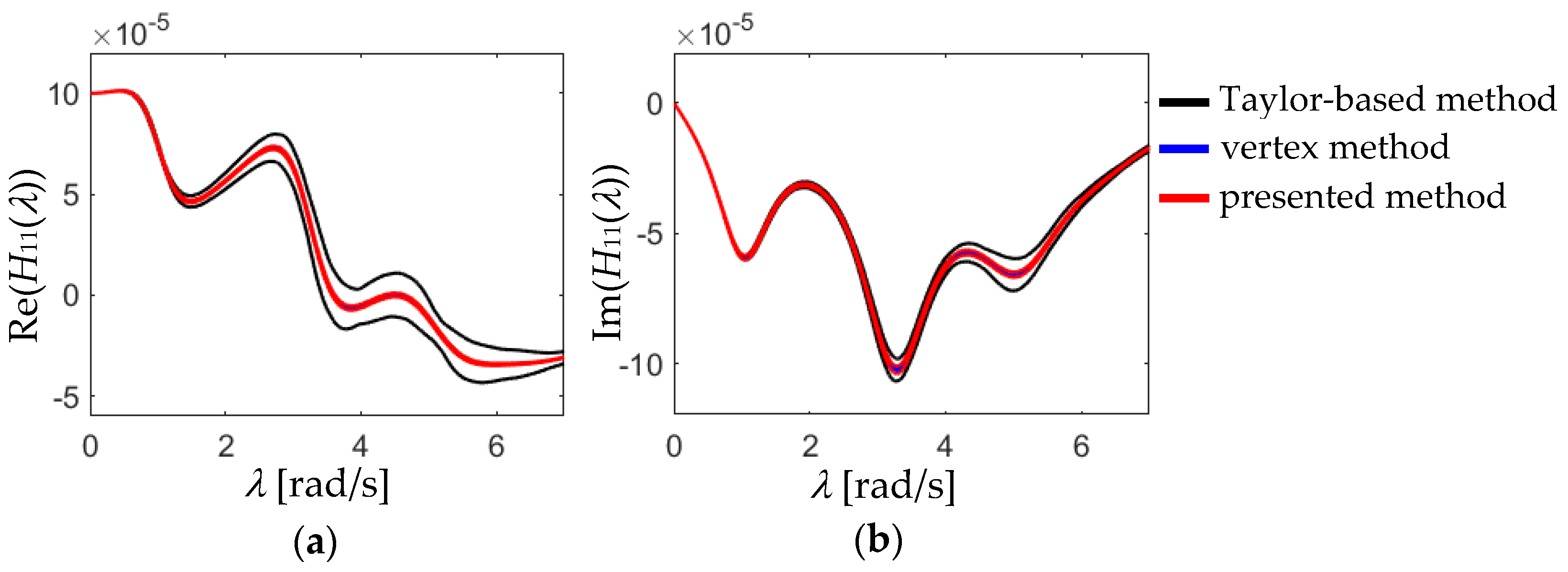
This paper presents a method for determining the dynamic response of systems with viscoelastic damping elements, where parameters are uncertain. It is assumed that uncertain parameters are described using interval numbers, meaning that the lower and upper bounds of the parameter are known. The presented method enables the consideration of uncertainties related to both the construction parameters and the damping elements, with a focus on demonstrating its applicability to parameters of viscoelastic material.

To determine the system’s dynamic response, interval analysis was applied. However, direct application can lead to the significant overestimation of results. To reduce this overestimation, equations of motion were formulated using the element-by-element technique, and a transformation was applied, ensuring uncertainties related to the same parameter are considered only once. This dual approach effectively reduces overestimation, as demonstrated in the provided examples. Additionally, all results were compared with those from the vertex method, known for its accuracy but being computationally intensive. The method used here involves solving linear interval equations via the fixed-point iteration method, utilizing Brower’s fixed-point theorem. It has been shown to yield satisfactory results at a considerably lower computational cost than the vertex method. However, it was observed that in cases of larger parameter variability (e.g., 10%), this iterative method may not always converge, necessitating the monitoring of convergence during computations. Nevertheless, as demonstrated in the examples with variability of 5%, the method produces accurate results and can effectively estimate the lower and upper bounds of the dynamic response of structures.

This method was applied for the first time to systems with viscoelastic elements described by both classical and fractional rheological models. Formulations were also proposed for both the Kelvin and Maxwell models. The Maxwell model, to be applicable with the presented method, requires a formulation with internal variables. The proposed approach is general and can be applied to more complex models, such as the Zener model or the generalized Maxwell model.

In future research, further reductions in overestimations, particularly in resonance zones, and improvements in method convergence in the case of larger uncertainties are planned. Additionally, the method is envisaged to be applied to the analysis of beams and plates with viscoelastic elements, which could have significant practical implications.

References

1. Ghanem, R.; Spanos, P.D. Stochastic Finite Elements; A Spectra Approach; Springer: New York, NY, USA, 1991. [Google Scholar]
2. Capillon, R.; Desceliers, C.; Soize, C. Uncertainty quantification in computational linear structural dynamics for viscoelastic composite structures. Comput. Methods Appl. Mech. Eng. 2016, 305, 154–172. [Google Scholar] [CrossRef]
3. Wang, T.; Xu, C.; Guo, N. A novel frequency-labeled adaptive sparse grid collocation method for uncertainty quantification of the frequency response of general viscoelastic damping structures. Int. J. Mech. Sci. 2021, 193, 106168. [Google Scholar] [CrossRef]
4. Jiang, C.; Liu, N.Y.; Ni, B.Y. A Monte Carlo simulation method for non-random vibration analysis. Acta Mech. 2017, 228, 2631–2653. [Google Scholar] [CrossRef]
5. Qiu, Z.P.; Wang, X. Vertex solution theorem for the upper and lower bounds on the dynamic response of structures with uncertain-but-bounded parameters. Acta Mech. Sin. 2009, 25, 367–379. [Google Scholar] [CrossRef]
6. Qiu, Z.P.; Wang, P.B. Parameter vertex method and its parallel solution for evaluating the dynamic response bounds of structures with interval parameters. Sci. China Phys. Mech. Astron. 2018, 61, 6–064612. [Google Scholar] [CrossRef]
7. Chen, S.H.; Lian, H.D.; Yang, X.W. Interval eigenvalue analysis for structures with interval parameters. Finite Elem. Anal. Des. 2003, 39, 419–431. [Google Scholar] [CrossRef]
8. Chen, S.H.; Lian, H.D. Dynamic response analysis for structures with interval parameters. Struct. Eng. Mech. 2002, 13, 299–312. [Google Scholar] [CrossRef]
9. Yang, X. Interval finite element method based on the element for eigenvalue analysis of structures with interval parameters. Struct. Eng. Mech. 2001, 12, 669–684. [Google Scholar] [CrossRef]
10. Qiu, Z.; Wang, X. Parameter perturbation method for dynamic responses of structures with uncertain-but-bounded parameters based on interval analysis. Int. J. Solids Struct. 2005, 42, 4958–4970. [Google Scholar] [CrossRef]
11. Xia, Y.; Qiu, Z.; Friswell, M.I. The time response of structures with bounded parameters and interval initial conditions. J. Sound Vib. 2010, 329, 353–365. [Google Scholar] [CrossRef]
12. Sim, J.; Qiu, Z.; Wang, X. Modal analysis of structures with uncertain-but-bounded parameters via interval analysis. J. Sound Vib. 2007, 303, 29–45. [Google Scholar] [CrossRef]
13. Moens, D.; Vandepitte, D. An interval finite element approach for the calculation of envelope frequency response functions. Int. J. Numer. Methods Eng. 2004, 61, 2480–2507. [Google Scholar] [CrossRef]
14. Yaowen, Y.; Zhenhan, C.; Yu, L. Interval analysis of dynamic response of structures using Laplace transform. Probabilist. Eng. Mech. 2012, 29, 32–39. [Google Scholar]
15. Muscolino, G.; Santoro, R.; Sofi, A. Explicit frequency response functions of discretized structures with uncertain parameters. Comput. Struct. 2014, 133, 64–78. [Google Scholar] [CrossRef]
16. Wei, T.; Li, F.; Meng, G. A bivariate Chebyshev polynomials method for nonlinear dynamic systems with interval uncertainties. Nonlinear Dyn. 2022, 107, 793–811. [Google Scholar] [CrossRef]
17. Qiu, Z.; Ma, L.; Wan, X. Non-probabilistic interval analysis method for dynamic response analysis of nonlinear systems with uncertainty. J. Sound Vib. 2009, 319, 531–540. [Google Scholar] [CrossRef]
18. Chen, S.H.; Ma, L.; Meng, G.W.; Guo, R. An efficient method for evaluating the natural frequencies of structures with uncertain-but-bounded parameters. Comput. Struct. 2009, 87, 582–590. [Google Scholar] [CrossRef]
19. Fujita, K.; Takewaki, I. An efficient methodology for robustness evaluation by advanced interval analysis using updated second-order Taylor series expansion. Eng. Struct. 2011, 33, 3299–3310. [Google Scholar] [CrossRef]
20. Łasecka-Plura, M.; Lewandowski, R. Dynamic characteristics and frequency response function for frame with dampers with uncertain design parameters. Mech. Based Des. Struct. Mach. 2017, 45, 296–312. [Google Scholar] [CrossRef]
21. Łasecka-Plura, M. Dynamic characteristics of a composite beam with viscoelastic layers under uncertain-but-bounded design parameters. Appl. Sci. 2023, 13, 6473. [Google Scholar] [CrossRef]
22. Kamiński, M.; Guminiak, M.; Lenartowicz, A.; Łasecka-Plura, M.; Przychodzki, M.; Sumelka, W. Stochastic nonlinear eigenvibrations of thin elastic plates resting on time-fractional viscoelastic supports. Probabilist. Eng. Mech. 2023, 74, 103522. [Google Scholar] [CrossRef]
23. Kamiński, M.; Guminiak, M.; Lenartowicz, A.; Łasecka-Plura, M.; Przychodzki, M.; Sumelka, W. Eigenvibrations of Kirchhoff rectangular random plates on time-fractional viscoelastic supports via stochastic finite element method. Materials 2023, 16, 7527. [Google Scholar] [CrossRef] [PubMed]
24. Muscolino, G.; Sofi, A. Stochastic analysis of structures with uncertain-but-bounded parameters via improved interval analysis. Probabilist. Eng. Mech. 2012, 28, 152–163. [Google Scholar] [CrossRef]
25. Wang, C.; Gao, W.; Song, C.; Zhang, N. Stochastic interval analysis of natural frequency and mode shape of structures with uncertainties. J. Sound Vib. 2014, 333, 2483–2503. [Google Scholar] [CrossRef]
26. Zhao, Y.; Deng, Z.; Han, Y. Dynamic response analysis of structure with hybrid random and interval uncertainties. Chaos Solit. Fractals 2020, 131, 109495. [Google Scholar] [CrossRef]
27. Feng, X.; Wu, J.; Zhang, Y. Time response of structure with interval and random parameters using a new hybrid uncertain analysis method. Appl. Math. Model. 2018, 64, 426–452. [Google Scholar] [CrossRef]
28. Zhao, D.; Zhou, X.; Wu, W. A metamodel-based multi-scale reliability analysis of FRP truss structures under hybrid uncertainties. Materials 2024, 17, 17010029. [Google Scholar] [CrossRef] [PubMed]
29. Sofi, A.; Muscolino, G.; Di Paola, M. Reliability analysis of structures controlled by external fractional viscoelastic dampers with interval parameters. Acta Mech. Sinica 2023, 39, 722486. [Google Scholar] [CrossRef]
30. Wang, L.; Wang, X.; Li, Y.; Lin, G.; Qiu, Z. Structural time-dependent reliability assessment of the vibration active control system with unknown-but-bounded uncertainties. Struct. Control Health Monit. 2016, 24, e1965. [Google Scholar] [CrossRef]
31. Fang, S.E.; Huang, J.Y. Statics-based model-free damage detection under uncertainties using modal interval analysis. Materials 2020, 13, 1567. [Google Scholar] [CrossRef]
32. Wang, L.; Zhou, L.; Liu, J. Interval-based optimal trajectory tracking control method for manipulators with clearance considering time-dependent reliability constraints. Aerosp. Sci. Technol. 2022, 128, 107745. [Google Scholar] [CrossRef]
33. Wang, L.; Liu, Y.; Li, Z.; Hu, J.; Han, B. Non-probabilistic reliability-based topology optimization (NRBTO) scheme for continuum structures based on the strength constraint parameterized level set method and interval mathematics. Thin-Walled Struct. 2023, 188, 110856. [Google Scholar] [CrossRef]
34. Liu, J.; Wang, L. Hybrid reliability-based sequential optimization for PID vibratory controller design considering interval and fuzzy mixed uncertainties. Appl. Math. Model. 2023, 122, 796–823. [Google Scholar] [CrossRef]
35. Moens, D.; Vandepitte, D. interval sensitivity theory and its application to frequency response envelope analysis of uncertain structures. Comput. Methods Appl. Mech. Engrg. 2007, 196, 2486–2496. [Google Scholar] [CrossRef]
36. Hernández, W.P.; Castello, D.A.; Ritto, T.G. Uncertainty propagation analysis in laminated structures with viscoelastic core. Comput. Struct. 2016, 164, 23–37. [Google Scholar] [CrossRef]
37. Hernández, W.P.; Castello, D.A.; Ritto, T.G. Stochastic fields to analyze uncertainties in laminated structures with viscoelastic core. J. Comput. Interdiscip. Sci. 2018, 9, 195–204. [Google Scholar]
38. Wang, T.; Xu, C.; Guo, N.; Hamdaoui, M.; Daya, E.I. Uncertainty propagation of frequency response of viscoelastic damping structures using a modified high-dimensional adaptive sparse grid collocation method. Mech. Adv. Mater. Struct. 2022, 29, 506–524. [Google Scholar] [CrossRef]
39. Nasab, M.S.E.; Kim, J. Fuzzy analysis of a viscoelastic damper in seismic retrofit of structures. Eng. Struct. 2022, 250, 113473. [Google Scholar] [CrossRef]
40. Nasab, M.S.E.; Guo, Y.Q.; Kim, J. Seismic retrofit of a soft first-story building using viscoelastic dampers considering inherent uncertainties. J. Build. Eng. 2022, 47, 103866. [Google Scholar] [CrossRef]
41. Lewandowski, R.; Litewka, P.; Łasecka-Plura, M.; Pawlak, Z.M. Dynamics of structures, frames, and plates with viscoelastic dampers or layers: A literature review. Buildings 2023, 13, 2223. [Google Scholar] [CrossRef]
42. Modares, M.; Mullen, R.L.; Muhanna, R.L. Natural frequencies of a structure with bounded uncertainty. J. Eng. Mech. 2006, 132, 1363–1372. [Google Scholar] [CrossRef]
43. Muhanna, R.L.; Zhang, H. Interval finite elements as a basis for generalized models of uncertainty in engineering mechanics. Reliab. Comput. 2007, 13, 173–194. [Google Scholar] [CrossRef]
44. Yaowen, Y.; Zhenhan, C.; Yu, L. Interval analysis of frequency response functions of structures with uncertain parameters. Mech. Res. Commun. 2013, 47, 24–31. [Google Scholar] [CrossRef]
45. Neumaier, A. Interval Methods for Systems of Equations; Cambridge University Press: New York, NY, USA, 1990. [Google Scholar]
46. Moore, R.E. Interval Analysis; Pretice Hall: Englewood Cliffs, NJ, USA, 1966. [Google Scholar]
47. Rump, S.M. On the solution of the interval linear systems. Computing 1992, 47, 337–353. [Google Scholar] [CrossRef]
48. Podlubny, I. Fractional Differential Equations; Academic Press: Cambridge, MA, USA, 1999. [Google Scholar]
49. Bagley, R.L.; Torvik, P.J. Fractional calculus—A different approach to the analysis of viscoelastically damped structures. AIAA J. 1983, 21, 741–748. [Google Scholar] [CrossRef]
50. Singh, M.P.; Chang, T.S.; Nandan, H. Algorithms for seismic analysis of MDOF systems with fractional derivatives. Eng. Struct. 2011, 33, 2371–2381. [Google Scholar] [CrossRef]
51. Lewandowski, R.; Pawlak, Z. Dynamic analysis of frames with viscoelastic dampers modelled by rheological models with fractional derivatives. J. Sound Vib. 2011, 330, 923–936. [Google Scholar] [CrossRef]
52. Lewandowski, R.; Bartkowiak, A.; Maciejewski, H. Dynamic analysis of frames with viscoelastic dampers: A comparison of damper models. Struct. Eng. Mech. 2012, 41, 13–37. [Google Scholar] [CrossRef]
53. Park, S.W. Analytical modeling of viscoelastic dampers for structural and vibration control. Int. J. Solids Struct. 2001, 38, 8065–8092. [Google Scholar] [CrossRef]
54. Hatada, T.; Kobori, T.; Ishida, M.; Niwa, N. Dynamic analysis of structures with Maxwell model. Eartquake Engng. Struct. Dyn. 2000, 29, 159–176. [Google Scholar] [CrossRef]
55. Chang, T.S.; Singh, M.P. Mechanical model parameters for viscoelastic dampers. J. Eng. Mech. 2009, 135, 581–584. [Google Scholar] [CrossRef]
56. Rump, S.M. Solving algebraic problems with high accuracy. In A New Approach to Scientific Computation; Kulish, U., Miranker, W., Eds.; Academic Press: New York, NY, USA, 1983; pp. 51–120. [Google Scholar]
57. Jansson, C. Interval linear system with symmetric matrices, skew-symmetric matrices, and dependencies in the right hand side. Computing 1991, 46, 265–274. [Google Scholar] [CrossRef]
58. Neumaier, A. Rigorous sensitivity analysis for parameter-dependent systems of equations. J. Math. Anal. Appl. 1989, 144, 14–25. [Google Scholar] [CrossRef]
59. Rump, S.M. Self-validating methods. Linear Algebra Appl. 2001, 324, 3–13. [Google Scholar] [CrossRef]
60. Rump, S.M. INTLAB—INTerval LABoratory. In Developments in Reliable Computing; Csendes, T., Ed.; Kluwer Academic Publishers: Dordrecht, The Netherlands, 1999; pp. 77–104. [Google Scholar]
61. Łasecka-Plura, M.; Lewandowski, R. Design sensitivity analysis of frequency response functions and steady-state response for structures with viscoelastic dampers. Vib. Phys. Syst. 2014, 26, 129–136. [Google Scholar]
Figure 1. Scott–Blair viscoelastic element.
Applsci 14 04556 g001
Figure 2. Models of viscoelastic elements: (a) classical Kelvin model; (b) fractional Kelvin model, (c) classical Maxwell model; (d) fractional Maxwell model.
Applsci 14 04556 g002
Figure 3. A frame with two Kelvin dampers.
Applsci 14 04556 g003
Figure 4. Single-DOF dynamic system: (a) with classical Kelvin damper; (b) with fractional Kelvin damper.
Applsci 14 04556 g004
Figure 5. Displacement plots—case 1: (a) real part; (b) imaginary part.
Applsci 14 04556 g005
Figure 6. Displacement plots—case 2: (a) real part; (b) imaginary part.
Applsci 14 04556 g006
Figure 7. Displacement plots—case 3: (a) real part; (b) imaginary part.
Applsci 14 04556 g007
Figure 8. Displacement plots—case 4: (a) real part; (b) imaginary part.
Applsci 14 04556 g008
Figure 9. Single-DOF dynamic system: (a) with classical Maxwell damper; (b) with fractional Maxwell damper.
Applsci 14 04556 g009
Figure 10. Displacement plots—case 1 without transformation (34): (a) real part; (b) imaginary part.
Applsci 14 04556 g010
Figure 11. Displacement plots—case 2 without transformation (34): (a) real part; (b) imaginary part.
Applsci 14 04556 g011
Figure 12. Displacement plots—case 1 with transformation (34): (a) real part; (b) imaginary part.
Applsci 14 04556 g012
Figure 13. Displacement plots—case 2 with transformation (34): (a) real part; (b) imaginary part.
Applsci 14 04556 g013
Figure 14. Four-story building with three dampers.
Applsci 14 04556 g014
Figure 15. Graphs of H11: (a) real part; (b) imaginary part.
Applsci 14 04556 g015
Figure 16. Graphs of H22: (a) real part; (b) imaginary part.
Applsci 14 04556 g016
Figure 17. Graphs of H33: (a) real part; (b) imaginary part.
Applsci 14 04556 g017
Figure 18. Graphs of H44: (a) real part; (b) imaginary part.
Applsci 14 04556 g018
Figure 19. Graphs of H11—uncertain dampers and structural parameters: (a) real part; (b) imaginary part.
Applsci 14 04556 g019
Figure 20. Graphs of H11 for parameter variability of 1%: (a) real part; (b) imaginary part.
Applsci 14 04556 g020
Figure 21. Graphs of H11 for parameter variability of 1%—zone 1: (a) real part; (b) imaginary part.
Applsci 14 04556 g021
Figure 22. Graphs of H11 for parameter variability of 1%—zone 2: (a) real part; (b) imaginary part.
Applsci 14 04556 g022
Figure 23. Graphs of H11 for parameter variability of 2%: (a) real part; (b) imaginary part.
Applsci 14 04556 g023
Figure 24. Graphs of H11: (a) real part; (b) imaginary part.
Applsci 14 04556 g024
Figure 25. Graphs of H22: (a) real part; (b) imaginary part.
Applsci 14 04556 g025
Figure 26. Graphs of H33: (a) real part; (b) imaginary part.
Applsci 14 04556 g026
Figure 27. Graphs of H44: (a) real part; (b) imaginary part.
Applsci 14 04556 g027