
Advancing Visible Spectroscopy through Integrated Machine Learning and Image Processing Techniques


Abstract
1. Introduction
2. Literature Review
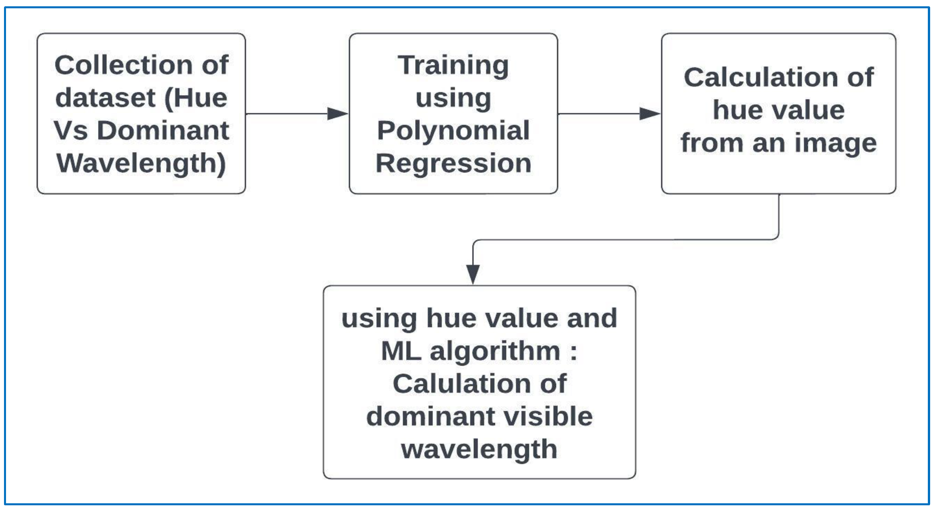
3. Methodology
4. Results and Discussions
5. Conclusions
Author Contributions
Funding
Data Availability Statement
Conflicts of Interest
References
- Milton, E.J.; Schaepman, M.E.; Anderson, K.; Kneubühler, M.; Fox, N. Progress in Field Spectroscopy. Remote Sens. Environ. 2009, 113, S92–S109. [Google Scholar] [CrossRef]
- John-Herpin, A.; Tittl, A.; Kühner, L.; Richter, F.; Huang, S.H.; Shvets, G.; Oh, S.; Altug, H. Metasurface-Enhanced Infrared Spectroscopy: An Abundance of Materials and Functionalities. Adv. Mater. 2022, 35, 2110163. [Google Scholar] [CrossRef]
- Pholpho, T.; Pathaveerat, S.; Sirisomboon, P. Classification of Longan Fruit Bruising Using Visible Spectroscopy. J. Food Eng. 2011, 104, 169–172. [Google Scholar] [CrossRef]
- Wang, N.; ElMasry, G. Bruise Detection of Apples Using Hyperspectral Imaging. In Hyperspectral Imaging for Food Quality Analysis and Control; Academic Press: Cambridge, MA, USA, 2010; pp. 295–320. [Google Scholar]
- Beberniss, T.J.; Ehrhardt, D.A. High-Speed 3D Digital Image Correlation Vibration Measurement: Recent Advancements and Noted Limitations. Mech. Syst. Signal Process. 2017, 86, 35–48. [Google Scholar] [CrossRef]
- Van Vliet, J.A.J.M.; De Groot, J.J. High-Pressure Sodium Discharge Lamps. IEE Proc. 1981, 128, 415. [Google Scholar] [CrossRef]
- Kitsinelis, S.; Devonshire, R.; Stone, D.A.; Tozer, R.C. Medium Pressure Mercury Discharge for Use as an Intense White Light Source. J. Phys. D Appl. Phys. 2005, 38, 3208–3216. [Google Scholar] [CrossRef]
- Trunec, D.; Brablec, A.; Buchta, J. Atmospheric Pressure Glow Discharge in Neon. J. Phys. D Appl. Phys. 2001, 34, 1697–1699. [Google Scholar] [CrossRef]
- Golubovskiǐ, Y.B.; Maйopoв, B.A.; Behnke, J.F.; Behnke, J.F. Modelling of the Homogeneous Barrier Discharge in Helium at Atmospheric Pressure. J. Phys. D Appl. Phys. 2002, 36, 39–49. [Google Scholar] [CrossRef]
- Amendola, V.; Meneghetti, M. Size Evaluation of Gold Nanoparticles by UV−vis Spectroscopy. J. Phys. Chem. C 2009, 113, 4277–4285. [Google Scholar] [CrossRef]
- Godiksen, A.; Vennestrøm, P.N.R.; Rasmussen, S.B.; Mossin, S. Identification and Quantification of Copper Sites in Zeolites by Electron Paramagnetic Resonance Spectroscopy. Top. Catal. 2016, 60, 13–29. [Google Scholar] [CrossRef]
- Windom, B.; Sawyer, W.G.; Hahn, D.W. A Raman Spectroscopic Study of MOS2 and MOO3: Applications to Tribological Systems. Tribol. Lett. 2011, 42, 301–310. [Google Scholar] [CrossRef]
- Rauscher, B.J.; Canavan, E.R.; Moseley, S.H.; Sadleir, J.E.; Stevenson, T. Detectors and Cooling Technology for Direct Spectroscopic Biosignature Characterization. J. Astron. Telesc. Instrum. Syst. 2016, 2, 041212. [Google Scholar] [CrossRef]
- Kurniastuti, I.; Yuliati, E.N.I.; Yudianto, F.; Wulan, T.D. Determination of Hue Saturation Value (HSV) Color Feature in Kidney Histology Image. J. Phys. Conf. Ser. 2022, 2157, 012020. [Google Scholar] [CrossRef]
- Cantrell, K.; Erenas, M.M.; de Orbe-Payá, I.; Capitán-Vallvey, L.F. Use of the Hue Parameter of the Hue, Saturation, Value Color Space As a Quantitative Analytical Parameter for Bitonal Optical Sensors. Anal. Chem. 2010, 82, 531–542. [Google Scholar] [CrossRef] [PubMed]
- Ma, M.; Gu, L.; Shen, Y.; Guan, Q.; Wang, C.; Deng, H.; Zhong, X.; Xia, M.; Shi, D. Computational Framework for Turbid Water Single-Pixel Imaging by Polynomial Regression and Feature Enhancement. IEEE Trans. Instrum. Meas. 2023, 72, 5021111. [Google Scholar] [CrossRef]
- Steinegger, A.; Wolfbeis, O.S.; Borisov, S. Optical Sensing and Imaging of pH Values: Spectroscopies, Materials, and Applications. Chem. Rev. 2020, 120, 12357–12489. [Google Scholar] [CrossRef] [PubMed]
- Wang, B.; Xu, H.; Jiang, G.; Yu, M.; Ren, T.; Luo, T.; Zhu, Z. UIE-ConvFormer: Underwater Image Enhancement Based on Convolution and Feature Fusion Transformer. IEEE Trans. Emerg. Top. Comput. Intell. 2024, 8, 1952–1968. [Google Scholar] [CrossRef]
- Simbolon, S.; Jumadi, J.; Khairil, K.; Yupianti, Y.; Yulianti, L.; Supiyandi, S.; Windarto, A.P.; Wahyuni, S. Image Segmentation Using Color Value of the Hue in CT Scan Result. J. Phys. Conf. Ser. 2022, 2394, 012017. [Google Scholar] [CrossRef]
- Garaba, S.P.; Friedrichs, A.; Voß, D.; Zielinski, O. Classifying Natural Waters with the Forel-Ule Colour Index System: Results, Applications, Correlations and Crowdsourcing. Int. J. Environ. Res. Public Health 2015, 12, 16096–16109. [Google Scholar] [CrossRef]
- Verma, M.; Yadav, V.; Kaushik, V.D.; Pathak, V.K. Multiple Polynomial Regression for Solving Atmospheric Scattering Model. Int. J. Adv. Intell. Paradig. 2019, 12, 400. [Google Scholar] [CrossRef]
- Kang, Z.; Fan, R.; Chen, Z.; Wu, Y.; Lin, Y.; Li, K.; Qu, R.; Xu, L. The Rapid Non-Destructive Differentiation of Different Varieties of Rice by Fluorescence Hyperspectral Technology Combined with Machine Learning. Molecules 2024, 29, 682. [Google Scholar] [CrossRef] [PubMed]
- Blake, N.; Gaifulina, R.; Griffin, L.D.; Bell, I.M.; Thomas, G.M.H. Machine Learning of Raman Spectroscopy Data for Classifying Cancers: A Review of the Recent Literature. Diagnostics 2022, 12, 1491. [Google Scholar] [CrossRef] [PubMed]
- Ede, J.M. Deep Learning in Electron Microscopy. Mach. Learn. Sci. Technol. 2021, 2, 011004. [Google Scholar] [CrossRef]
- Goodacre, R. Explanatory Analysis of Spectroscopic Data Using Machine Learning of Simple, Interpretable Rules. Vib. Spectrosc. 2003, 32, 33–45. [Google Scholar] [CrossRef]
- Li, L.; Zhang, Q.; Ding, Y.; Jiang, H.; Thiers, B.H.; Wang, J. Automatic Diagnosis of Melanoma Using Machine Learning Methods on a Spectroscopic System. BMC Med. Imaging 2014, 14, 36. [Google Scholar] [CrossRef] [PubMed]
- Rodellar, J.; Alférez, S.; Acevedo, A.; Molina, Á.; Merino, A. Image Processing and Machine Learning in the Morphological Analysis of Blood Cells. Int. J. Lab. Hematol. 2018, 40, 46–53. [Google Scholar] [CrossRef]
- Carey, C.; Boucher, T.; Mahadevan, S.; Dyar, M.D.; Bartholomew, P. Machine Learning Tools for Mineral Recognition and Classification from Raman Spectroscopy. J. Raman Spectrosc. 2014, 1783, 5053. [Google Scholar] [CrossRef]
- Zeng, C.; Yan, Y.; Tang, J.; Wu, Y.; Zhong, S. Speciation of Arsenic(III) and Arsenic(V) Based on Triton X-100 Hollow Fiber Liquid Phase Microextraction Coupled with Flame Atomic Absorption Spectrometry. Spectrosc. Lett. 2017, 50, 220–226. [Google Scholar] [CrossRef]
- Bai, F.; Fan, Z. Flow Injection Micelle-Mediated Methodology for Determination of Lead by Electrothermal Atomic Absorption Spectrometry. Mikrochim. Acta 2007, 159, 235–240. [Google Scholar] [CrossRef]
- Li, X.; Liu, Z.; Cui, S.; Luo, C.; Li, C.; Zhuang, Z. Predicting the Effective Mechanical Property of Heterogeneous Materials by Image Based Modeling and Deep Learning. Comput. Methods Appl. Mech. Eng. 2019, 347, 735–753. [Google Scholar] [CrossRef]
- Zhang, P.; Liu, B.; Mu, X.; Xu, J.; Du, B.; Wang, J.; Liu, Z.; Tong, Z. Performance of Classification Models of Toxins Based on RAMAN Spectroscopy Using Machine Learning Algorithms. Molecules 2023, 29, 197. [Google Scholar] [CrossRef] [PubMed]
- Kruse, F.A.; Lefkoff, A.B.; Boardman, J.W.; Heidebrecht, K.B.; Shapiro, A.T.; Barloon, P.J.; Goetz, A. The Spectral Image Processing System (SIPS)—Interactive Visualization and Analysis of Imaging Spectrometer Data. Remote Sens. Environ. 1993, 44, 145–163. [Google Scholar] [CrossRef]
- Yang, Q.; Tian, S.; Xu, H. Identification of the Geographic Origin of Peaches by VIS-NIR Spectroscopy, Fluorescence Spectroscopy and Image Processing Technology. J. Food Compos. Anal. 2022, 114, 104843. [Google Scholar] [CrossRef]
- Simon, L.L.; Nagy, Z.K.; Hungerbühler, K. Comparison of External Bulk Video Imaging with Focused Beam Reflectance Measurement and Ultra-Violet Visible Spectroscopy for Metastable Zone Identification in Food and Pharmaceutical Crystallization Processes. Chem. Eng. Sci. 2009, 64, 3344–3351. [Google Scholar] [CrossRef]
- Vong, C.N.; Larbi, P.A. Comparison of Image Data Obtained with Different Commercial Cameras for Use in Visible Spectroscopy. In Proceedings of the 2016 ASABE Annual International Meeting, Orlando, FL. USA, 17–20 July 2016. [Google Scholar] [CrossRef]
- Liŭ, D.; Sun, D.; Zeng, X. Recent Advances in Wavelength Selection Techniques for Hyperspectral Image Processing in the Food Industry. Food Bioprocess Technol. 2013, 7, 307–323. [Google Scholar] [CrossRef]
- Plaza, A.; Benediktsson, J.A.; Boardman, J.W.; Brazile, J.; Bruzzone, L.; Camps-Valls, G.; Chanussot, J.; Fauvel, M.; Gamba, P.; Gualtieri, A.G.; et al. Recent Advances in Techniques for Hyperspectral Image Processing. Remote Sens. Environ. 2009, 113, S110–S122. [Google Scholar] [CrossRef]
- Yonezawa, K.; Takahashi, M.; Yatabe, K.; Nagatani, Y.; Shimizu, N. MOLASS: Software for Automatic Processing of Matrix Data Obtained from Small-Angle X-Ray Scattering and UV–Visible Spectroscopy Combined with Size-Exclusion Chromatography. Biophys. Physicobiol. 2023, 20, e200001. [Google Scholar] [CrossRef]
- Grasse, E.K.; Torcasio, M.H.; Smith, A.W. Teaching UV–Vis Spectroscopy with a 3D-Printable Smartphone Spectrophotometer. J. Chem. Educ. 2015, 93, 146–151. [Google Scholar] [CrossRef]
- Green, R.O.; Eastwood, M.L.; Sarture, C.M.; Chrien, T.G.; Aronsson, M.; Chippendale, B.J.; Faust, J.; Pavri, B.; Chovit, C.; Solis, M.; et al. Imaging Spectroscopy and the Airborne Visible/Infrared Imaging Spectrometer (AVIRIS). Remote Sens. Environ. 1998, 65, 227–248. [Google Scholar] [CrossRef]
- Shakya, J.R.; Shashi, F.H.; Wang, A.X. Plasmonic Color Filter Array Based Visible Light Spectroscopy. Sci. Rep. 2021, 11, 23687. [Google Scholar] [CrossRef]
- Usami, M.; Iwamoto, T.; Fukasawa, R.; Tani, M.; Watanabe, M.; Sakai, K. Development of a THz Spectroscopic Imaging System. Phys. Med. Biol. 2002, 47, 3749–3753. [Google Scholar] [CrossRef] [PubMed]
- Delaney, J.K.; Zeibel, J.G.; Thoury, M.; Littleton, R.T.; Morales, K.M.; Palmer, M.R.; De La Rie, E.R. Visible and Infrared Reflectance Imaging Spectroscopy of Paintings: Pigment Mapping and Improved Infrared Reflectography. In Proceedings of the SPIE, Munich, Germany, 7 July 2009. [Google Scholar] [CrossRef]
- Ktash, M.A.; Hauler, O.; Ostertag, E.; Brecht, M. Ultraviolet-Visible/near Infrared Spectroscopy and Hyperspectral Imaging to Study the Different Types of Raw Cotton. J. Spectr. Imaging 2020, 9, 1–11. [Google Scholar] [CrossRef]
- Baka, N.A.; Abu-Siada, A.; Islam, S.; El-Naggar, M. A New Technique to Measure Interfacial Tension of Transformer Oil Using UV-Vis Spectroscopy. IEEE Trans. Dielectr. Electr. Insul. 2015, 22, 1275–1282. [Google Scholar] [CrossRef]
- Haffert, S.Y.; Males, J.R.; Close, L.M.; Van Gorkom, K.; Long, J.D.; Hedglen, A.D.; Guyon, O.; Schatz, L.; Kautz, M.; Lumbres, J.; et al. The Visible Integral-field Spectrograph eXtreme (VIS-X): High-resolution spectroscopy with MagAO-X. arXiv 2022, arXiv:2208.02720. [Google Scholar]
- Van der Woerd, H.J.; Wernand, M.R. Hue-Angle Product for Low to Medium Spatial Resolution Optical Satellite Sensors. Remote Sens. 2018, 10, 180. [Google Scholar] [CrossRef]
- Wikipedia Contributors Sodium-Vapor Lamp. Available online: https://en.wikipedia.org/wiki/Sodium-vapor_lamp (accessed on 7 April 2024).
- Wikipedia Contributors Gas-Discharge Lamp. Available online: https://en.wikipedia.org/wiki/Gas-discharge_lamp (accessed on 7 April 2024).
- Xometry, T. Copper Vapor Laser: Definition, Importance, and How It Works. Available online: https://www.xometry.com/resources/sheet/copper-vapor-laser/#:~:text=A%20copper%20vapor%20laser%20is,temperatures%20required%20to%20vaporize%20copper%20lamp (accessed on 7 April 2024).
- Atomic Spectra. Available online: http://hyperphysics.phy-astr.gsu.edu/hbase/quantum/atspect.html (accessed on 7 April 2024).
- Wikipedia Contributors Mercury-Vapor Lamp. Available online: https://en.wikipedia.org/wiki/Mercury-vapor_lamp (accessed on 7 April 2024).

| Feature | Specification |
|---|---|
| Technique | Atomic Absorption Spectroscopy (AAS) |
| Wavelength Range | 190 nm to 900 nm |
| Spectral Bandwidth | 0.1, 0.2, 0.4, 1.0, 2.0 nm (selectable) |
| Wavelength Accuracy | ±0.25 nm |
| Wavelength Repeatability | ±0.15 nm |
| Baseline Drift | ≤0.005 Abs/30 min |
| Background Correction | Deuterium lamp background correction |
| Atomisation Methods | Flame Atomiser, Graphite Furnace Atomiser |
| Heating temperature range (Graphite Furnace) | Room temperature~2650 °C |
| Lamp Type | Hollow Cathode Lamp (HCL) |
| Number of Lamp Positions | 8 (automatic turret) |
| Sample Types | Liquids, Solids |
| Precision (RSD) | ≤3% |
| Software Compatibility | Windows Platform |
| Steps | Code | Comment |
|---|---|---|
| 1. | X_train, X_test, y_train, y_test = train_test_split (X, Y, test_size = 0.2, random_state = 0) | Splitting the data into training and testing sets |
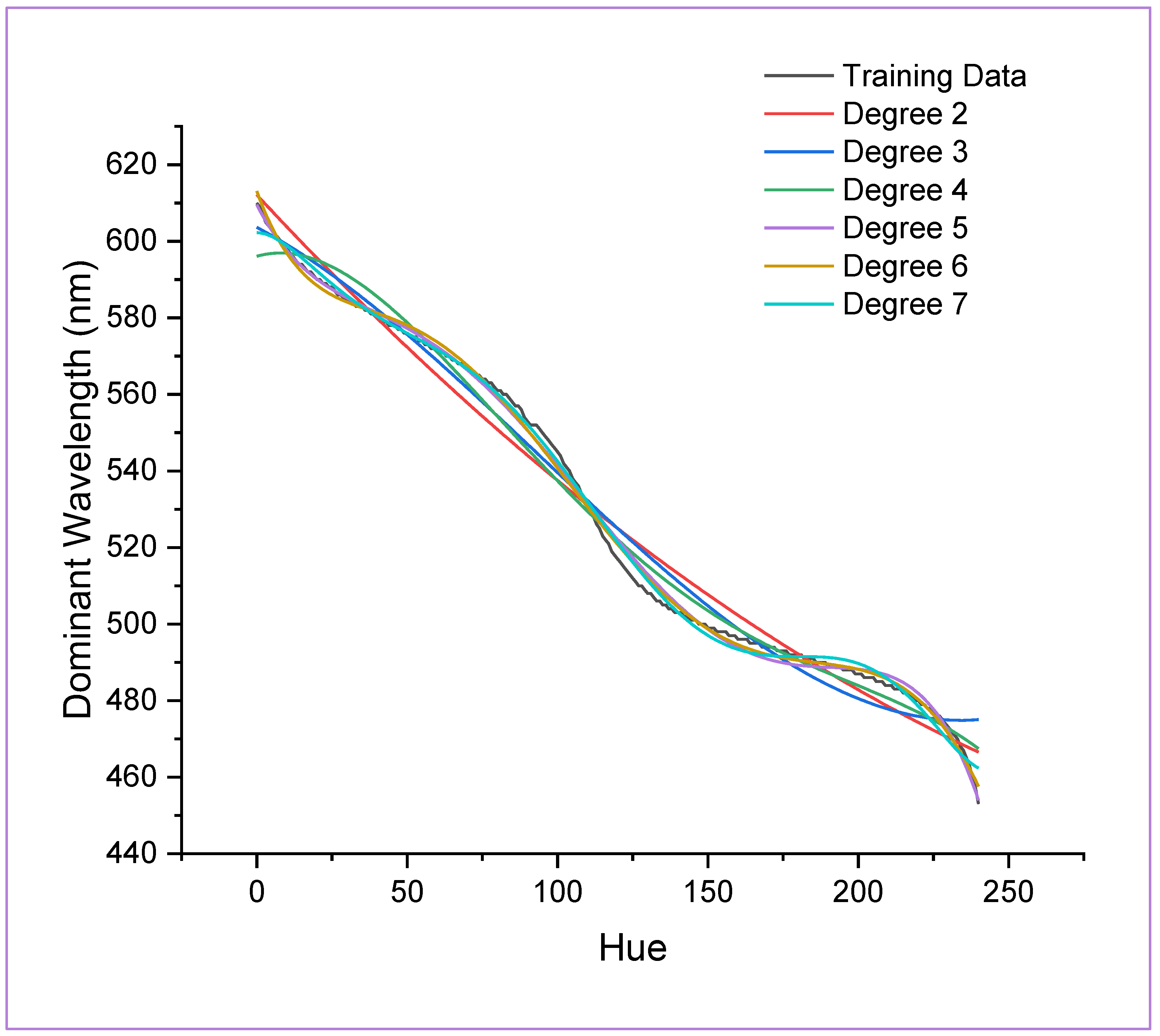
| 2. | poly_reg = PolynomialFeatures (degree = 6) | Creating polynomial features with specified degree |
| 3. | X_poly = poly_reg.fit_transform (X_train) | Transforming the training features into polynomial features |
| 4. | pol_reg = LinearRegression () | Initialising linear regression model |
| 5. | pol_reg.fit (X_poly, y_train) | Fitting the polynomial features to the target variable |
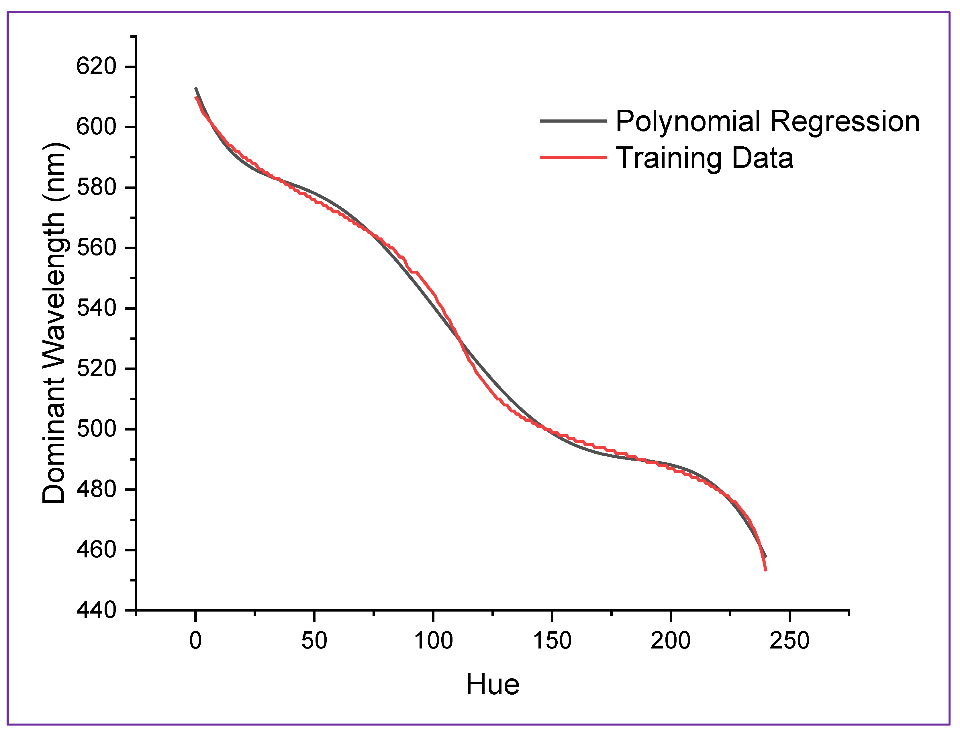
| Hue | Training Data [48] | Polynomial Regression | Hue | Training Data [48] | Polynomial Regression | Hue | Training Data [48] | Polynomial Regression |
|---|---|---|---|---|---|---|---|---|
| 0 | 610 | 613.13 | 81 | 561 | 558.97 | 162 | 496 | 493.99 |
| 1 | 609 | 611.02 | 82 | 560 | 558.10 | 163 | 496 | 493.70 |
| 2 | 607 | 609.04 | 83 | 560 | 557.22 | 164 | 495 | 493.42 |
| 3 | 605 | 607.17 | 84 | 559 | 556.32 | 165 | 495 | 493.16 |
| 4 | 604 | 605.42 | 85 | 558 | 555.41 | 166 | 495 | 492.90 |
| 5 | 603 | 603.76 | 86 | 557 | 554.49 | 167 | 495 | 492.67 |
| 6 | 602 | 602.21 | 87 | 557 | 553.56 | 168 | 494 | 492.44 |
| 7 | 601 | 600.75 | 88 | 556 | 552.62 | 169 | 494 | 492.23 |
| 8 | 600 | 599.39 | 89 | 554 | 551.67 | 170 | 494 | 492.03 |
| 9 | 599 | 598.10 | 90 | 553 | 550.72 | 171 | 494 | 491.84 |
| 10 | 598 | 596.90 | 91 | 552 | 549.75 | 172 | 494 | 491.66 |
| 11 | 597 | 595.78 | 92 | 552 | 548.77 | 173 | 493 | 491.49 |
| 12 | 596 | 594.73 | 93 | 552 | 547.79 | 174 | 493 | 491.33 |
| 13 | 595 | 593.75 | 94 | 551 | 546.80 | 175 | 493 | 491.18 |
| 14 | 594 | 592.83 | 95 | 550 | 545.81 | 176 | 493 | 491.04 |
| 15 | 594 | 591.97 | 96 | 549 | 544.81 | 177 | 492 | 490.91 |
| 16 | 593 | 591.17 | 97 | 548 | 543.80 | 178 | 492 | 490.78 |
| 17 | 592 | 590.43 | 98 | 547 | 542.79 | 179 | 492 | 490.66 |
| 18 | 592 | 589.73 | 99 | 546 | 541.78 | 180 | 492 | 490.54 |
| 19 | 591 | 589.08 | 100 | 545 | 540.76 | 181 | 492 | 490.43 |
| 20 | 590 | 588.47 | 101 | 544 | 539.75 | 182 | 491 | 490.33 |
| 21 | 590 | 587.90 | 102 | 542 | 538.73 | 183 | 491 | 490.23 |
| 22 | 589 | 587.37 | 103 | 541 | 537.71 | 184 | 491 | 490.13 |
| 23 | 589 | 586.88 | 104 | 540 | 536.69 | 185 | 491 | 490.03 |
| 24 | 588 | 586.41 | 105 | 538 | 535.67 | 186 | 490 | 489.93 |
| 25 | 588 | 585.97 | 106 | 537 | 534.65 | 187 | 490 | 489.84 |
| 26 | 587 | 585.56 | 107 | 536 | 533.63 | 188 | 490 | 489.74 |
| 27 | 586 | 585.17 | 108 | 534 | 532.61 | 189 | 490 | 489.64 |
| 28 | 586 | 584.81 | 109 | 533 | 531.60 | 190 | 489 | 489.54 |
| 29 | 585 | 584.46 | 110 | 531 | 530.59 | 191 | 489 | 489.44 |
| 30 | 585 | 584.12 | 111 | 530 | 529.59 | 192 | 489 | 489.33 |
| 31 | 584 | 583.80 | 112 | 528 | 528.59 | 193 | 489 | 489.22 |
| 32 | 584 | 583.50 | 113 | 526 | 527.59 | 194 | 489 | 489.10 |
| 33 | 583 | 583.20 | 114 | 525 | 526.60 | 195 | 488 | 488.97 |
| 34 | 583 | 582.91 | 115 | 523 | 525.62 | 196 | 488 | 488.83 |
| 35 | 583 | 582.63 | 116 | 522 | 524.64 | 197 | 488 | 488.69 |
| 36 | 582 | 582.35 | 117 | 521 | 523.67 | 198 | 488 | 488.53 |
| 37 | 582 | 582.07 | 118 | 519 | 522.71 | 199 | 487 | 488.37 |
| 38 | 581 | 581.79 | 119 | 518 | 521.76 | 200 | 487 | 488.19 |
| 39 | 581 | 581.52 | 120 | 517 | 520.81 | 201 | 487 | 488.00 |
| 40 | 580 | 581.24 | 121 | 516 | 519.88 | 202 | 486 | 487.79 |
| 41 | 580 | 580.96 | 122 | 515 | 518.96 | 203 | 486 | 487.57 |
| 42 | 579 | 580.67 | 123 | 514 | 518.04 | 204 | 486 | 487.33 |
| 43 | 579 | 580.38 | 124 | 513 | 517.14 | 205 | 486 | 487.07 |
| 44 | 578 | 580.08 | 125 | 512 | 516.25 | 206 | 485 | 486.79 |
| 45 | 578 | 579.78 | 126 | 511 | 515.37 | 207 | 485 | 486.50 |
| 46 | 578 | 579.46 | 127 | 510 | 514.51 | 208 | 485 | 486.18 |
| 47 | 577 | 579.14 | 128 | 510 | 513.66 | 209 | 484 | 485.84 |
| 48 | 577 | 578.80 | 129 | 509 | 512.82 | 210 | 484 | 485.47 |
| 49 | 576 | 578.45 | 130 | 508 | 511.99 | 211 | 484 | 485.08 |
| 50 | 576 | 578.09 | 131 | 508 | 511.18 | 212 | 483 | 484.67 |
| 51 | 575 | 577.72 | 132 | 507 | 510.38 | 213 | 483 | 484.23 |
| 52 | 575 | 577.34 | 133 | 506 | 509.60 | 214 | 483 | 483.76 |
| 53 | 575 | 576.93 | 134 | 506 | 508.83 | 215 | 482 | 483.25 |
| 54 | 574 | 576.52 | 135 | 505 | 508.07 | 216 | 482 | 482.72 |
| 55 | 574 | 576.09 | 136 | 505 | 507.34 | 217 | 481 | 482.16 |
| 56 | 573 | 575.64 | 137 | 504 | 506.61 | 218 | 481 | 481.56 |
| 57 | 573 | 575.18 | 138 | 504 | 505.91 | 219 | 480 | 480.93 |
| 58 | 572 | 574.70 | 139 | 503 | 505.22 | 220 | 480 | 480.26 |
| 59 | 572 | 574.20 | 140 | 503 | 504.54 | 221 | 479 | 479.56 |
| 60 | 572 | 573.69 | 141 | 503 | 503.89 | 222 | 479 | 478.82 |
| 61 | 571 | 573.16 | 142 | 502 | 503.25 | 223 | 478 | 478.04 |
| 62 | 571 | 572.61 | 143 | 502 | 502.62 | 224 | 478 | 477.21 |
| 63 | 570 | 572.04 | 144 | 501 | 502.02 | 225 | 477 | 476.35 |
| 64 | 570 | 571.46 | 145 | 501 | 501.43 | 226 | 476 | 475.44 |
| 65 | 569 | 570.86 | 146 | 501 | 500.86 | 227 | 476 | 474.49 |
| 66 | 569 | 570.24 | 147 | 500 | 500.30 | 228 | 475 | 473.49 |
| 67 | 568 | 569.61 | 148 | 500 | 499.76 | 229 | 474 | 472.45 |
| 68 | 568 | 568.95 | 149 | 500 | 499.24 | 230 | 473 | 471.36 |
| 69 | 567 | 568.28 | 150 | 499 | 498.74 | 231 | 472 | 470.22 |
| 70 | 567 | 567.60 | 151 | 499 | 498.25 | 232 | 471 | 469.03 |
| 71 | 566 | 566.89 | 152 | 499 | 497.78 | 233 | 470 | 467.79 |
| 72 | 566 | 566.17 | 153 | 498 | 497.33 | 234 | 468 | 466.49 |
| 73 | 565 | 565.43 | 154 | 498 | 496.89 | 235 | 467 | 465.15 |
| 74 | 565 | 564.68 | 155 | 498 | 496.48 | 236 | 465 | 463.74 |
| 75 | 564 | 563.91 | 156 | 498 | 496.07 | 237 | 463 | 462.29 |
| 76 | 564 | 563.12 | 157 | 497 | 495.69 | 238 | 460 | 460.77 |
| 77 | 563 | 562.32 | 158 | 497 | 495.32 | 239 | 457 | 459.20 |
| 78 | 563 | 561.51 | 159 | 497 | 494.96 | 240 | 453 | 457.57 |
| 79 | 562 | 560.68 | 160 | 496 | 494.62 | |||
| 80 | 561 | 559.83 | 161 | 496 | 494.30 |
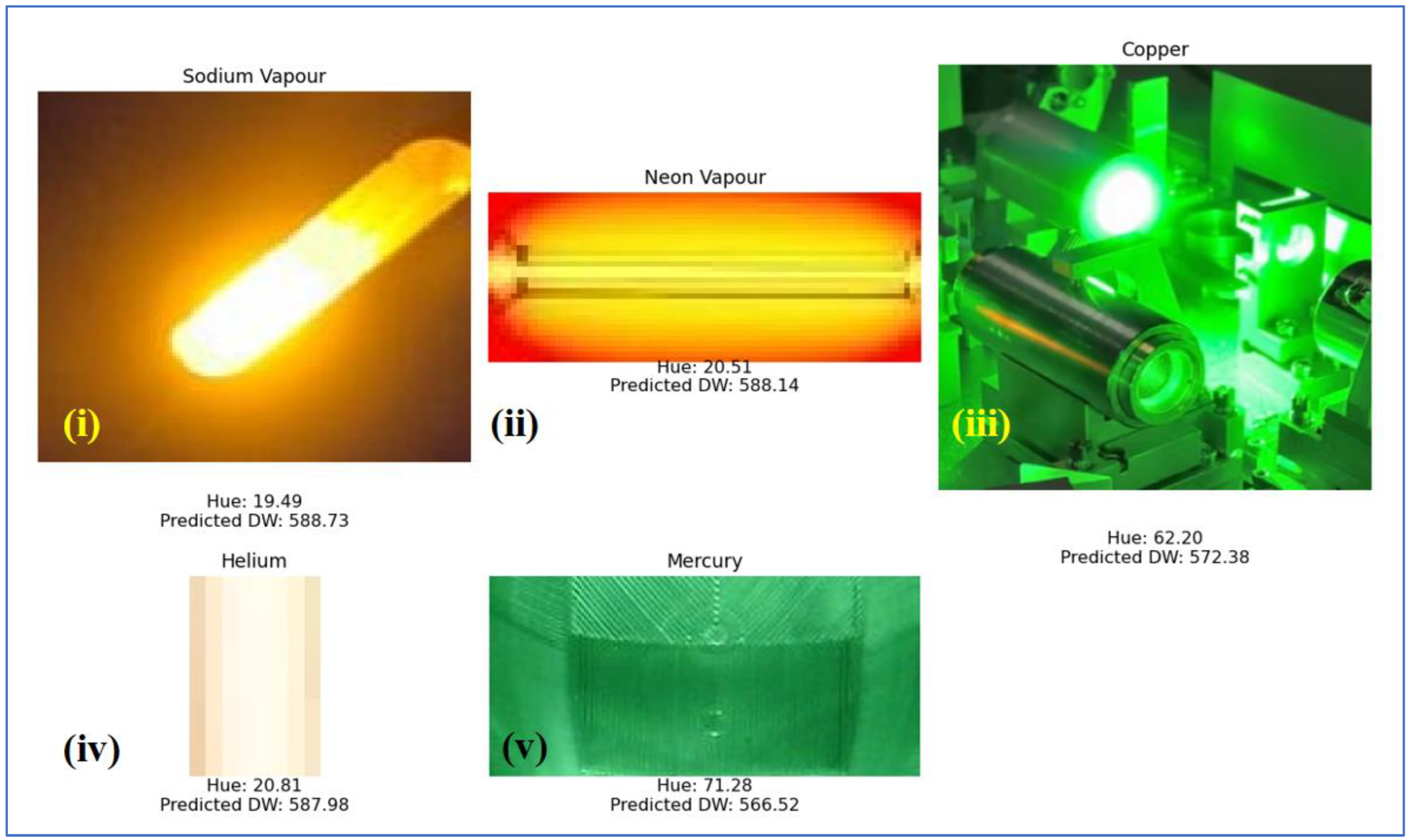
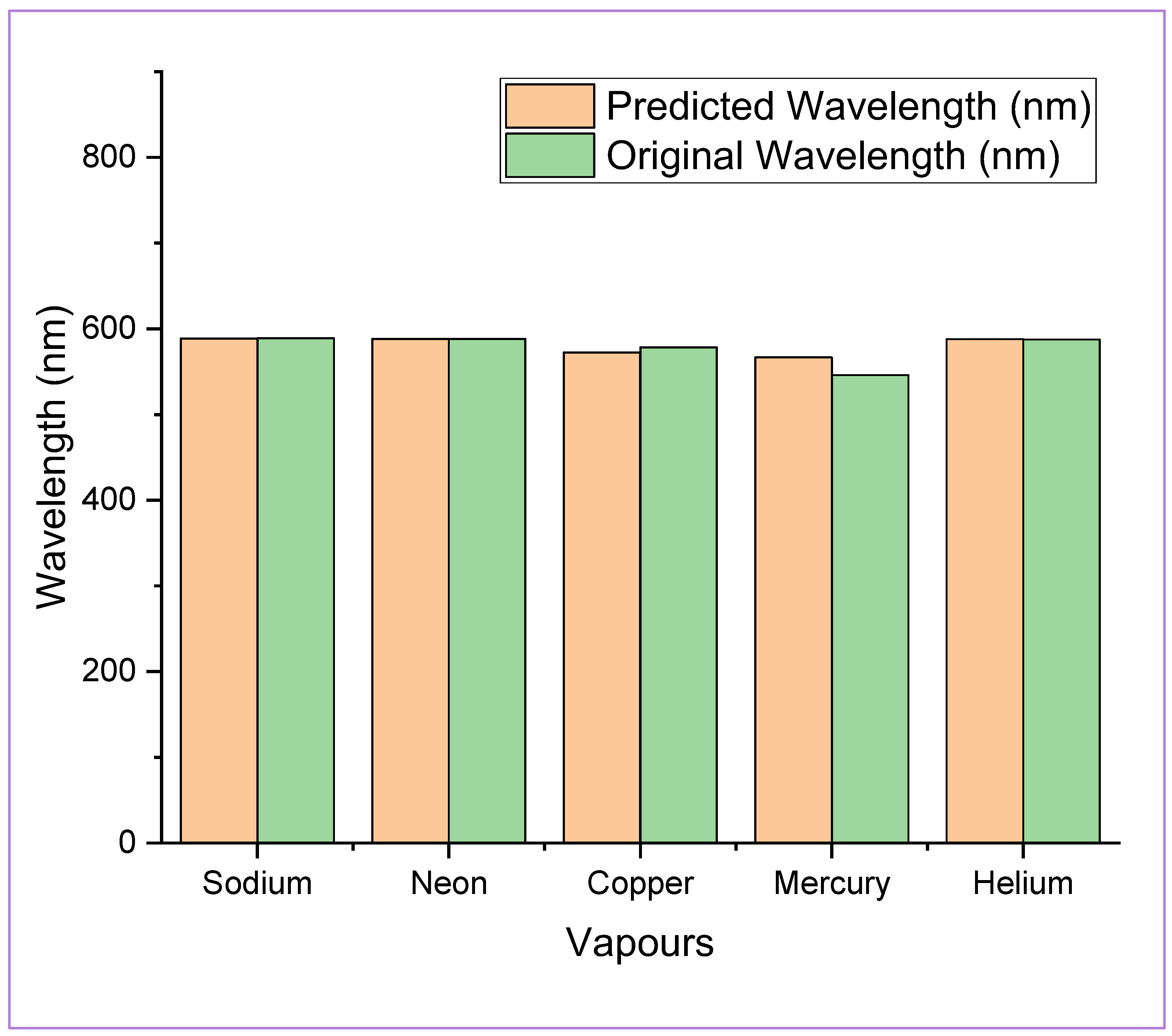
| Vapour | Predicted Wavelength (nm) | Original Wavelength (nm) | Error Percentage |
|---|---|---|---|
| Sodium | 588.73231 | 589 | 0.04% |
| Neon | 588.14 | 588.2 | 0.01% |
| Copper | 572.38412 | 578.2 | 1% |
| Mercury | 566.5212 | 546.074 | 3.7% |
| Helium | 587.97620 | 587.562 | 0.07% |
Disclaimer/Publisher’s Note: The statements, opinions and data contained in all publications are solely those of the individual author(s) and contributor(s) and not of MDPI and/or the editor(s). MDPI and/or the editor(s) disclaim responsibility for any injury to people or property resulting from any ideas, methods, instructions or products referred to in the content. |
© 2024 by the authors. Licensee MDPI, Basel, Switzerland. This article is an open access article distributed under the terms and conditions of the Creative Commons Attribution (CC BY) license (https://creativecommons.org/licenses/by/4.0/).
Share and Cite
Patra, A.; Kumari, K.; Barua, A.; Pradhan, S. Advancing Visible Spectroscopy through Integrated Machine Learning and Image Processing Techniques. Appl. Sci. 2024, 14, 4527. https://doi.org/10.3390/app14114527
Patra A, Kumari K, Barua A, Pradhan S. Advancing Visible Spectroscopy through Integrated Machine Learning and Image Processing Techniques. Applied Sciences. 2024; 14(11):4527. https://doi.org/10.3390/app14114527
Chicago/Turabian StylePatra, Aman, Kanchan Kumari, Abhishek Barua, and Swastik Pradhan. 2024. "Advancing Visible Spectroscopy through Integrated Machine Learning and Image Processing Techniques" Applied Sciences 14, no. 11: 4527. https://doi.org/10.3390/app14114527
APA StylePatra, A., Kumari, K., Barua, A., & Pradhan, S. (2024). Advancing Visible Spectroscopy through Integrated Machine Learning and Image Processing Techniques. Applied Sciences, 14(11), 4527. https://doi.org/10.3390/app14114527