Traffic Flow Prediction with Random Walks on Graph and Spatiotemporal Bidirectional Attention Transformer

Abstract

Traffic flow prediction is crucial in intelligent transportation systems. Considering the severe disruptions caused by traffic accidents or congestion, a time series model is developed for traffic flow prediction based on multiple random walks on graphs (MRWG) and the bidirectional spatiotemporal attention mechanism (BSAM), which can adapt to both normal and exceptional situations. The MRWG mechanism is applied to capture spatial features of urban areas during traffic accidents and congestion, especially the spatial dependencies among neighboring regions. Further, a local position attention module is applied to acquire the spatial correlations between different regions to investigate their impact on the global area, while a local temporal attention module is adopted to extract short-term periodic time correlations from traffic flow data. Finally, a spatiotemporal bidirectional attention module is applied to simultaneously extract both the temporal and spatial correlations of the historical traffic flow data in order to generate the output prediction. Experiments have been conducted on NYCTaxi and NYCBike datasets with abnormal events, and the results indicate that the developed model can efficiently predict traffic flow in abnormal events, especially short-term traffic disruptions, outperforming the baseline methods under both abnormal and normal conditions.

1. Introduction

With the rapid development of new technologies and urbanization, the number of vehicles in the global transportation sector has increased sharply, which makes the operation of the urban transportation networks face greater pressure in terms of infrastructure capacity and environmental sustainability. Therefore, accurate traffic prediction in urban areas plays an important role in the management of intelligent transportation systems (TIS) [1,2] that can guide individuals to avoid congested routes, saving travel time and reducing greenhouse gas emission [3,4]. The extensive research on traffic flow prediction suggests that a transportation system can be categorized into two scenarios when modelling traffic flow, namely general conditions and abnormal conditions, whereas the prediction models in turn can be classified into statistical models [5], shallow machine learning models [6], and deep learning algorithms [7] in the current transport modeling studies.

A thorny issue arising from the statistical theory-based methods [8,9,10,11] and machine learning-based approaches [12,13,14] is that these models have struggled to capture the high-dimensional spatiotemporal features in the historical data. With deep learning methods demonstrating advantages in capturing the hidden nonlinear relationships embedded in the existing data, they can be applied to predict the traffic flow with satisfied performance. As the LSTM (Long-Short Term Memory) network has the advantages of dealing with time series data, it has gradually been used for traffic flow prediction. An LSTM Neural Network (LSTM-NN) is developed to extract the nonlinear dynamics in the traffic historical data [15], while a deep bidirectional uni-directional stacked LSTM-NN architecture considers the forward and backward dependencies of the traffic flow data to predict the network flow speed [16]. However, these LSTM-based methods only model the temporal relationships of traffic flow data, without considering the inherent spatial relationship in those data. Therefore, convolution neural networks [17] or deep residual convolutional structures [18] are employed to capture the spatial correlations in the data. However, either spatial or temporal correlations of the data have extensively been considered individually in the existing studies, leading to suboptimal prediction performance in complex traffic flow data.

Convolutional Neural Networks (CNN) and LSTM can be combined together for traffic flow prediction, considering both temporal and spatial correlations simultaneously [19]. The city-into-regions and a CNN-based end-to-end spatiotemporal residual network is developed to extract the spatiotemporal correlation among different regions [20]. A multi-view spatiotemporal network is developed where a CNN is employed to learn the local spatial correlations under shared similar temporal patterns [21]. However, the spatial information is easily removed or neglected by the global average pooling layer in the CNN, and the short-term temporal correlation is also twisted and cannot be considered continuously via the long-term dependency of the recursive network. Graph-based deep learning methods have been applied to capture the dependencies in non-Euclidean spaces. Examples include Graph Convolutional Networks (GCN) [22] and Graph Attention [23], which can encode the topological network of road traffic by integrating the graph-based LSTM and CNN structures, thereby enhancing the spatiotemporal correlations. Cui et al. have proposed a traffic graph convolutional LSTM-NN to model the traffic network as a graph and embed the traffic flow network into the graph so as to enhance the prediction accuracy [24]. A deep learning framework with a dynamic spatial-temporal graph convolutional network has been proposed to capture the dynamic spatial and temporal dependencies simultaneously, and an attention mechanism is incorporated to dynamically learn weights between traffic nodes based on graph features together with dilated causal convolution to capture the long-term tendencies of traffic data [25].

However, the impact of exceptional events, i.e., traffic accidents or congestion, on traffic flow prediction has seldom been considered, while the dissipation of spatiotemporal correlation features within the depth of the network are also not taken into account in their modeling framework.

The occurrence of abnormal events on a road could lead to significant deviations in traffic patterns as the traffic conditions during such periods are more dependent on instantaneous variations. In such scenarios, they can be classified into two categories: (1) long-term and planned events, such as weekday rush hours and holidays; (2) short-term unexpected events, including traffic accidents, adverse weather conditions, temporary traffic controls, etc. Hence, real-world traffic data can be used, while similarity features among regions are used as the spatial information [26] and contextual data locations, weather conditions, and traffic accidents are useful for the traffic flow prediction with improved prediction performance [27].

Shallow machine learning methods (in contrast to deep learning) can be adopted for traffic prediction under accidental conditions. For instance, an online regression support vector machine model (RSVR) has been proposed with higher performance with respect to traffic flow prediction in holiday and traffic accident scenarios [28]. Guo et al. [29] have developed a traffic predictor based on KNN (k-nearest neighbors) combined with singular spectrum analysis technology to predict short-term traffic flow via an integrated gradient lifting regression tree. Further, Chen et al. [30] have conducted traffic flow prediction in the short term via integrated gradient lifting regression trees. However, these methods only directly use traffic data under abnormal conditions or varied conditions without explicitly modeling the spatiotemporal impact of the local abnormal events on traffic flow.

Yu et al. [31] extracted the temporal correlation of multi-scale traffic flow by stacking LSTM networks and used the stacked autoencoders to extract the potential feature representations under peak periods and traffic accidents. Jiang et al. [32] designed an encoder and decoder architecture via ConvLSTM to predict citywide crowd dynamics during major events (e.g., earthquakes, national holidays). Liu et al. [33] designed a spatiotemporal convolutional sequence learning architecture based on accident encoding, which can effectively capture the short-term spatiotemporal correlations via unidirectional convolution, and it employs a self-attention mechanism to obtain long-term spatiotemporal periodic correlations.

To extract the complicated spatiotemporal correlations efficiently, Huang et al. [34] have proposed an encoder–decoder model for multi-step output prediction based on the bidirectional attention mechanism and multi-head spatial attention mechanism. The model uses bidirectional attention flows to investigate the intricate spatiotemporal correlations between the prediction data and historical data, predicting real-time ride-hailing demand during the COVID-19 pandemic. Luo et al. [35] have developed a Multi-Task Multi-Range Multi-Subgraph Attention Network (M3AN) which can be adaptable for both normal and abnormal traffic situations. Different subgraphs are used to model node attributes while attention mechanisms are employed to measure the dynamic spatial correlations. However, most current condition-aware traffic-prediction methods fall short of meeting expectations.

It is noted that various abnormal events (i.e., type, duration, and intensity) also impact traffic conditions across areas. For example, traffic congestion in one region could cause congestion in adjacent regions with comparable traffic change patterns. However, these changes in similar patterns could vary over time, indicating diverse spatial correlations. Spatiotemporal correlations between metropolitan regions are complicated within a given time frame, and precise traffic flow prediction necessitates extracting the spatiotemporal correlations of different locations at various time intervals.

We suggest a seq2seq model called multiple random walks on graphs BiAttenn (MRWG BiAtten), which combines multiple random walks on graphs and bidirectional spatiotemporal attention mechanisms for traffic flow prediction under abnormal events, to tackle these difficulties. The contributions of the manuscript are summarized as follows:

(1)

A traffic flow-prediction model based on Transformer is proposed with the applied encoder–decoder structure to integrate the graph random walk and spatiotemporal bidirectional attention mechanisms, in light of the impact of traffic accidents and congestion on urban traffic conditions.

(2)

A positional attention module is introduced allowing simultaneous concentration on both global and local spatial links by aggregating the global spatial correlations on local spatial features.

(3)

To enable the extraction of intricate and dynamic temporal dependencies, a time attention module is proposed to model the interdependencies between the long-term and short-term temporal features.

(4)

Two baseline datasets, TaxiNYC and BikeNYC, are used in the experiments for performance comparison to verify the superiority of the proposed prediction model.

The remainder of the paper is organized as follows. Section 2 introduces the problem formulation, and Section 3 describes the proposed traffic flow-prediction model in detail. In Section 4, in-depth experiments with public traffic datasets are carried out to validate the performance of the proposed model. Conclusions are provided in Section 5.

2. Problem Formulation

Certain symbols are first defined for the traffic flow-prediction problem formulation, where the traffic flow in the temporal dimension is frequently a continuation of the historical traffic flow states with periodicity.

The entire city can be represented as a $U\times V$ grid, with N regions ($N=U\times V$); $S=\{s_1,s_2,\cdots ,s_r\}$ denotes each region, and $T=\{t_1,t_2,\cdots ,t_n\}$ represents the entire time span of the historical observed data. The MRWG model is demonstrated in Figure 1, including an encoder and a decoder, which can be used to predict the traffic flow volume. $Q_{out}=\left\{Q_i^{t^{\prime }}\right|i\in [0,\cdots ,N-1],t^{\prime }\in T,\cdots ,T+l-1\}$ in urban areas l time stamps into the future based on historical traffic flow dataset $\{E_i^t\in R^{T\times u\times v}|i\in [0,\cdots ,N-1],t\in [0,\cdots ,T-1]\}$. Here, $E_i^t$ records the traffic flow volume in each urban area during the historical time period $t$, and $Q_i^{t^{\prime }}$ represents the predicted traffic flow volume for each urban area at future time stamps $t^{\prime }$.

When processing the spatial and temporal correlations in the historical traffic flow data, sudden occurrences of traffic accidents or congestion from one area to another would cause a rapid spread of local traffic states to the surrounding areas after they have been maintained for some time [36]. Furthermore, different types of abnormal accidents have varied effects on the traffic conditions in the surrounding regions.

Given the historical traffic flow data of the target region and the abnormal events Y, the surrounding region $B$ subgraphs are formed based on the total abnormal event types. The historical traffic flow data are divided into B groups (the same as regions), denoted as $\kappa =\left\{{\kappa }_1,{\kappa }_2,\cdots ,{\kappa }_B\right\}$. Considering the historical traffic flow and transient data $E_{in}\in R^{T\times U\times V}$ and $Q_{in}\in R^{T\times U\times V}$, as well as the accident data $\kappa$, the traffic flow prediction can be formalized as a learning function $f_{\theta }$ that maps the input to the output prediction of the traffic flow $\stackrel{⌢}{Y}$ at the next timestep:

$$\stackrel{⌢}{Y}=f_{\theta }(E_{in},Q_{in},\kappa )$$

(1)

where $\stackrel{⌢}{Y}\in R^{l\times U\times V}$ and $\theta$ represent the predicted traffic flow and learnable parameters, respectively.

3. The Proposed Traffic Flow-Prediction Model

The developed encoder–decoder model structure is depicted in Figure 1. The input sequence ($E_{in}$) is the historical traffic flow data which enter the encoder to capture the spatiotemporal features in the representation tensor ($E_{en}$), then they enter into the decoder along with supplementary information $Q_{in}=Q_{tj}|j\in [n,\cdots ,n+l-1]$ to produce an output sequence ($Q_{out}$) of the future traffic flow status. Here, Q_tj represents the predicted results for each grid during time period t_j. Next, the encoder and decoder are formally described in detail.

(1)

Encoder: Four layers are included in the encoder: a Local CNN layer, an MH-SSA layer (multi-position attention machine layer), an FC-FF layer (fully connected feed-forward network layer), and a residual connection [37] with a Norm layer [38]. Here, E_in is the input of the encoder and E_en is the encoded output.

(2)

Decoder: The structure of the decoder is similar to that of the encoder, consisting of a Local CNN layer, double-attention mechanism layers (dotted brown rectangle), an FC-FF layer and a Norm layer. The first layer of the attention mechanism (blue-filled rectangle in Figure 1) is the MT-SSA layer, which takes the output $Q_{de}^0$ of the Local CNN layer as input to obtain the spatiotemporal feature Q_de. The second layer is the BiAtten layer (green-filled rectangle in Figure 1), which takes E_en and Q_de as the inputs to calculate the bidirectional attention matrix $H_{de}^1$ and $U_{de}^1$. After the FC-FF layer and Norm layer, the decoded states can be obtained as H_de and U_de.

3.1. The Random Walk Mechanism Based on Multi-Graph Attention

To thoroughly investigate the impact of traffic accidents and congestion, the regions of a city are encoded where abnormal traffic events occurred at the same time intervals so as to extract the positional features and spatial details of the abnormal traffic events. Next, the encoded regional graph is subjected to a multi-graph attention mechanism to dynamically model the spatial correlations of various kinds of abnormal events, as local subgraphs. When the captured abnormal traffic events occur between regions, the spatial features can be captured via the introduced attention mechanism to especially focus on the common variations in the traffic data across regions after the occurrence of the same type of abnormal event. Therefore, spatiotemporal features can be extracted via the multi-graph attention mechanism with the random walk mechanism. When traffic anomalies occur in the future, the random walk mechanism can account for the local and global traffic flow changes in the urban regional network.

(1)

Location coding

Map coding is applied [29] to extract the future location of the abnormal traffic events, representing potential traffic congestion. The coded location is used as the location accident information, and the event location feature $b_i^t$ is represented as the one-hot vector $b_i^{\prime t}\in R^{v+\beta }$, where v is the amount of time intervals. Let $\beta =N$ represent the number of urban areas. Thus, the accident location coding $b_i^t$ can be embedded in $A{E}^i\in R^{T\times (v+\beta )}$,

$$A{E}_t^i=f({\mu }_{t,1}^i\cdot \mathrm{Re}LU({\mu }_{t,0}^i{b^{\prime }}_t^i+d_{t,0}^i)+d_{t,1}^i)$$

(2)

where $f(\cdot )$ is an activation function and $\left\{{\mu }_{t,0}^i,d_{t,0}^i,{\mu }_{t,1}^i,d_{t,1}^i\right\}$ are the learnable parameters in different layers of the network.

(2)

Multiple subgraph attention modules

According to the location feature AEⁱ, the subgraph B is formed via the historical traffic data $\kappa =\left\{{\kappa }_1,{\kappa }_2,\cdots ,{\kappa }_B\right\}$. Then, the historical traffic data from various regions with the same abnormal event type at different time steps are aggregated as a virtual node v, and the node subset (V_b) is constructed with K neighboring regions. Then, the traffic flow data are integrated into subgraph B via the Graph Attention (GAT) block as [39],

$$S_{vi,v,b}=a(<W_{b}h{l}_{vi,b}^{l-1}\cdot W_{b}h{l}_{v,b}^{l-1}>)$$

(3)

$${\alpha }_{vi,v,b}=\frac{\exp (s_{vi,v,b})}{{\displaystyle {\sum }_{vr\in V_b}\exp (s_{vi,v,b})}}$$

(4)

$$h{l}_{vi,b}^{(l)}={\displaystyle \sum _{v\in V_b}{\alpha }_{vi,v,b}}h{l}_{vi,b}^{l-1}$$

(5)

where vi is the hidden state of the node, denoted as $h{l}_{vi,b}^{(l-1)}$, representing the b^th GAT block ($1\le b\le B$); $s_{vi,v,b}$ represents the correlation coefficient between node v and the adjacent node vi; W_b is the hyper-parameter of the b^th graph. $‖\cdot ‖$ denotes the concatenation operation; $<\cdot ,\cdot >$ represents the inner product; $a(\cdot )$ is a single-layer feed-forward neural network which maps the concatenated high-dimensional features to a real number. For the b^th GAT block, the output of the multi-subgraph attention module is represented as ${\chi }_{ms,b}\in R^{P\times U\times V}$.

Considering the highly dynamic characteristics of the traffic flow conditions in the accident-prone regions, the impact on the traffic flow of the surrounding areas varies along with time and different types of ambient events. Here, the output of the multi-subgraph attention module is used with a random walk mechanism (RWA) to adaptively capture the correlations among various neighboring target nodes at low computational cost, improving the system ability to adapt to local variations in different abnormal event locations.

3.2. The Attention Mechanism Layer

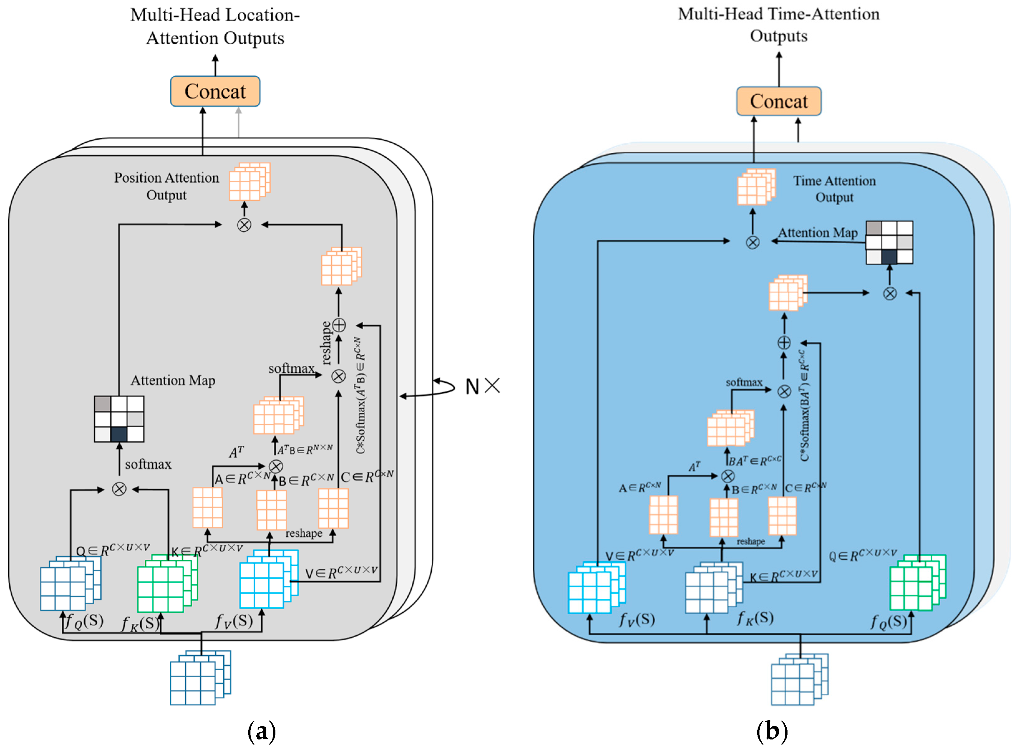
The attention mechanism layer consists of the MH-SSA layer (multi-position attention layer), the MT-SSA layer (multi-time attention layer), and the BiAtten layer (the spatiotemporal bidirectional attention layer). Figure 2 depicts the configuration of the MH-SSA layer and the MT-SSA layer.

(1)

The multi-position attention module

A location attention module is introduced in the encoder to extract the spatial correlation between potential local and global regions in the traffic flow history data. The location attention module weights all the location features based on similarities between regions in order to focus on both the local spatial correlation and global spatial correlations at the same time.

As shown in Figure 2a, given a historical dataset $A\in R^{C\times U\times V}$, it is passed through a convolutional layer so as to generate two new feature maps B and C, i.e., $\left\{B,C\right\}\in R^{C\times U\times V}$. Further, they are reshaped into $R^{C\times N}$, and $N=U\times V$ is the amount of city regions. Then, matrix C is multiplied by the transpose of B, and the spatial positional attention map $S\in R^{N\times N}$ is calculated via the sofmax function,

$$s_{ij}=\frac{\exp (B_i\cdot C_j)}{{\displaystyle {\sum }_{i=1}^N\exp (B_i\cdot C_j)}}$$

(6)

where S_ij is the impact of position i on position j. The greater the similarity of the feature representations, the greater the correlation between the two locations.

In the meantime, feature A is input into the convolution layer, and a new feature map D is generated and reshaped into R. The transpositions of D are multiplied by S and then the result is reshaped into R as well. Afterwards, the reshaped result is multiplied with the scaling parameter $\alpha$ and summed up piecewise to obtain the final output,

$$E_j=\alpha {\displaystyle \sum _{i=1}^N(s_{ji}{D}_i)}+A_j$$

(7)

where $\alpha$ is the learning parameter with initial value 0 [28]. From Equation (7), it can be obtained that feature E is the weighted sum of the global spatial correlation features and local spatial correlation, and similar regional spatial correlations are mutually enhanced accordingly. Then, E is used as a value matrix to participate in the calculation of the attention matrix.

(2)

The multi-temporal attention module

A temporal attention module is designed to capture the long-term and short-term temporal periodical correlation from historical traffic flow data. The module emphasizes the interrelated long-term time features to improve the short-term time-dependent feature representation, shown in Figure 2b. Unlike the location-attention module, the temporal attention graph $X\in R^{C\times C}$ is calculated from the history traffic flow data $A\in R^{C\times U\times V}$. $A$ is reshaped to $A\in R^{C\times N}$, $N=U\times V$, then the time attention map $X\in R^{C\times C}$ is obtained via the softmax layer:

$$x_{ij}=\frac{\exp (A_i\cdot A_j)}{{\displaystyle {\sum }_{i=1}^C\exp (A_i\cdot A_j)}}$$

(8)

where $x_{ij}$ represents the impact of the i^th timestamp on the j^th timestamp. Subsequently, matrix multiplication is performed between X and the transpose of A to capture the periodicity in the long term, reshaping the result into $R^{C\times U\times V}$. Then the standard parameter $\eta$ is applied with the obtained results and the final output $K\in R^{C\times U\times V}$ can be obtained with the element-wise summation of the original data A:

$$K_j=\eta {\displaystyle \sum _{i=1}^C(x_{ji}{A}_i)}+A_j$$

(9)

where $\eta$ is the learnable weight with initial value 0. Equation (9) indicates that the final feature of each timestamp is a weighted summation of the periodic features of all timestamps with the correlation features of short-term timestamps. Then K is used as a key matrix to participate in the calculation of the attention matrix.

(3)

The bidirectional spatiotemporal attention module

Inspired by the design of the BiDAF network [40], the decoder includes a bidirectional spatiotemporal attention module designed to handle both the historical data (E_en) and predicted data (Q_de). To combine the spatial correlation features from the location attention module (LAM) with temporal correlation features from the temporal attention module (TAM), it computes a set of attention feature vectors. Following that, the spatiotemporal bidirectional attention features are computed at each timestamp, based not only on the features from the previous time step but also the interactions of all traffic flow situations.

In this module, the input consists of the spatial correlation features $E_{en}={[e^0,\cdots ,e^i,\cdots ,e^{k-1}]}^T\in R^{k\times U\times V}$ and $Q_{de}={[q^0,\cdots ,q^j,\cdots ,q^{l-1}]}^T\in R^{l\times U\times V}$. We compute the attention scores from both directions, $E_{en}$ to $Q_{de}$ and $Q_{de}$ to $E_{en}$, for the calculations, i.e., $H_{de}^1={[h_{UV}^0,\cdots ,h_{UV}^i,\cdots ,h_{UV}^{k-1}]}^T\in R^{k\times UV}$ the historical spatiotemporal awareness vector and the predicted spatiotemporal awareness vector $U_{de}^1={[u_{UV}^0,\cdots ,u_{UV}^i,\cdots ,u_{UV}^{k-1}]}^T\in R^{l\times UV}$.

(4)

The multi-output strategy

The MRWG BiAtten model can be used to predict the future traffic demand for all regions, thus maintaining the spatiotemporal correlations between regions and prediction time intervals. Inspired by the design of the BiDAF network [40], the integrated attention vectors $H_{de}^1$, $U_{de}^1$, the processed decoder states $H_{de}$, $U_{de}$, and the encoder states $E_{en}$ are all combined together,

$$G=[E_{en};U_{de};E_{en}\circ U_{de};E_{en}\circ H_{de}]\in R^{4l\times UV}$$

(10)

where “◦” denotes the element-wise multiplication and [;] represents the concatenation of the cross columns. $G$ is then transformed to obtain the final result $Q_{out}\in R^{l\times UV}$ via a one-dimensional CNN, where each column of $Q_{out}$ can be assumed as the predicted representation of each input of the historical regional traffic data.

4. Experiment and Result Analysis

4.1. Data Acquisition and Processing

The performance of the proposed MRWG BiAtten model is examined on two datasets, i.e., the BikeNYC dataset and the TaxiNYC dataset. Both datasets are associated with traffic flow demand, including time, region, demand request times, etc. In addition, motor vehicle accident data of New York City (NYC) are added to analyze the impact of abnormal events. The NYC dataset consists of the traffic records of in total 60 days in 2016, including 8000 traffic accidents per month, where each record contains the location of the vehicles and the start and end times of the journey.

Table 1. Dataset details.

Dataset	TaxiNYC	BikeNYC
Time duration	1 January 2016–29 February 2016	1 July 2016–29 August 2016
Sampling interval	15 min	15 min
City region scope	10 × 20	10 × 20
Vehicle number	24,000+	8200+
Max flow	928	168
Total records	23 million	3.2 million

is a summary of the two datasets.

The first 45 days of the dataset are used as the training data, and the remainder for the test set. Before the training, min-max scaling is used to unify the data in the range of [0, 1], and the prediction output is de-normalized for evaluation. The Local CNN networks have a space pool size of m = 7, a {7 × 7} convolution kernel. In our proposed model, the dropout rate is set to d_prate = 0.1, and the number of stacked model layers and N multi-head attention modules is set as 4 and 8, respectively. The performed hardware environment contains 1 × NVIDIA GeForce RTX 3080(10G) GPUs and 2 × Intel Xeon Silver 4214R CPU. The learning rate is set as 0.001 and the batch size is fixed as 64. The training epoch is set as 500 to ensure convergence and the Adam optimizer is used to train the model.

4.2. Data Analysis and Evaluation Metrics

In order to verify the prediction performance of the proposed method, the root mean square error (RMSE) and mean absolute error (MAE) are used as the evaluation indexes:

$$RMSE=\sqrt{\frac{1}{n}{\displaystyle \sum _{i=1}^n{(y_i-{\widehat{y}}_i)}^2}}$$

(11)

$$MAE=\frac{1}{n}{\displaystyle \sum _{i=1}^n\left|y_i-{\widehat{y}}_i\right|}$$

(12)

where $y_i$ and ${\widehat{y}}_i$ represent the actual and predicted traffic flow, respectively; n is the number of traffic zones.

Several prediction models are used for comparison, HA, ARIMA, LSTM, ConvLSTM, and STDN (Spatiotemporal Dynamic Network). These methods can be divided into three categories: (1) traditional statistics-based time series prediction model (HA, ARIMA); (2) time series prediction model based on deep learning (LSTM); (3) deep learning network for traffic flow prediction based on spatiotemporal feature mining (ConvLSTM, STDN). The details of these comparison methods are described below.

4.3. Comparison Experiments and Analysis

The test results with the two datasets are listed in

Table 2. Comparison results conducted on BikeNYC and TaxiNYC datasets.

Methods	BikeNYC				TaxiNYC
	Inflow		Outflow		Inflow		Outflow
	RMSE	MAE	RMSE	MAE	RMSE	MAE	RMSE	MAE
HA	11.28	8.30	10.56	7.86	25.94	17.22	23.26	14.86
ARIMA	27.80	23.44	27.71	23.54	52.2	33.32	46.34	34.26
LSTM	9.85	6.96	9.42	6.86	19.76	13.55	16.56	12.01
ConvLSTM	9.73	6.82	9.42	6.81	18.26	12.79	16.27	11.20
STDN	8.75	5.98	8.21	6.22	16.92	10.85	15.42	8.76
Our method	7.92	5.85	7.83	6.12	16.37	10.13	14.86	8.34

. The MAE and RMSE of TaxiNYC are higher than those of BikeNYC, as the data scale of TaxiNYC is larger than that of BikeNYC. In both metrics, the statistical time series analysis methods HA and ARIMA have significantly larger prediction deviations than that of the LSTM method for both datasets. This indicates that manually extracting the temporal features cannot precisely obtain the nonlinear temporal correlations in traffic data.

We take inflow data as an example. On the BikeNYC dataset, the ConvLSTM method has a lower RMSE and MAE than LSTM by 1.22% and 2.01%, respectively. On the TaxiNYC dataset, ConvLSTM outperforms LSTM with 7.59% lower RMSE and 5.61% lower MAE. This suggests that spatial and temporal correlations are more effective than temporal correlations alone, emphasizing the significance of modeling spatial dependencies between regions.

On the BikeNYC dataset, we take the inflow data as an example, where our proposed approach outperforms ConvLSTM by 18.59% and 14.22%, and STDN by 9.49% and 2.17%, when it comes to capturing spatial and short-term/long-term temporal correlations. On the TaxiNYC dataset, our proposed method can achieve lower RMSE and MAE compared to ConvLSTM by 10.35% and 20.79%, and compared to STDN by 3.25% and 6.64%.

It is noteworthy that STDN with an attention mechanism outperforms the ConvLSTM model. This observation confirms that the attention mechanism can be used to enhance the capability of spatiotemporal feature extraction. Our approach is designed with a multi-head position attention module for extracting spatial features, which includes a multi-head time attention module to extract the temporal features and a bidirectional attention module to extract both the temporal and spatial features. This allows our model to have superior spatiotemporal prediction capability compared to the baseline models.

The suboptimal performance of ConvLSTM may be attributed to its incapacity to completely exploit the potential spatiotemporal correlations in traffic flow data. Therefore, in order to improve the prediction accuracy, STDN makes an effort to capture spatial correlations as well as short- and long-duration temporal correlations via multi-perspective and long-term attention processes. However, the prediction accuracy is lower than that of the MRWG BiAtten due to the omitted effects of other events, including accidents in traffic flow.

Our approach utilizes a random walk method based on a multi-graph attention mechanism to encode the accident data as spatial features to depict traffic congestion, and performs much better than the networks without the accident-encoding structure. As indicated in

Table 3. Analysis of the role of the accident module.

Dataset	Method	With Acc	No Acc
		RMSE	RMSE
TaxiNYC	LSTM	18.58	18.75
	ConvLSTM	18.88	18.75
	STDN	16.47	16.93
	Our method	16.28	16.51
BikeNYC	LSTM	9.54	9.46
	ConvLSTM	9.35	9.45
	STDN	8.34	8.61
	Our method	7.98	8.42

, the role of accident data in traffic flow prediction is evaluated via RMSE. The right two columns indicate whether the accident data module is considered; the majority of the aforementioned techniques perform better when the accident data are taken into account, particularly for models which take spatial correlations into account. It is seen that the proposed model can achieve the best improvement since the accident data are incorporated via the random walk method based on a multi-graph attention mechanism. However, LSTM, due to its focus only on the temporal features, performs poorly in extracting spatial relationships from external features, indicating that accident data can be used to extract useful local semantic information variations and apply them to traffic flow prediction.

4.4. Sensitivity Analysis

The sensitivity of the proposed MRWG BiAtten model is analyzed. Figure 3a demonstrates that the RMSE error first drops then rises with the increase in attention layers performed on the BikeNYC inflow dataset, and the MAE error has a similar tendency. Therefore, moderately increasing the network depth can increase the prediction accuracy. However, it could face overfitting or other issues if the network is too deep, which can explain the reason that the RMSE error increases with more than four attention layers. Figure 3b shows that the model also behaves similarly on the TaxiNYC inflow dataset.

Within the constraints of the specified attention head count, we have explored the impact of different numbers of heads. Figure 4 depicts the RMSE and MAE values on the BikeNYC and TaxiNYC datasets as the number of attention heads varies. The results indicate that, when the number of the attention heads is set to less than 8, both RMSE and MAE values gradually decrease with the increase in the attention head count. However, once the count exceeds 8, RMSE and MAE values begin to rise, suggesting that appropriately increasing the number of attention heads can enhance the performance. Nevertheless, exceeding a certain number may lead to overfitting.

Eventually, the best prediction performance is achieved when all components are combined together. As displayed in Figure 5, high prediction accuracy can be obtained in most regions with high proportion, indicating that the model performs satisfactorily in traffic flow prediction.

There are two main reasons that the MRWG BiAtten model works better than the alternative methods: (1) The MRWG BiAtten model uses the position attention mechanism to capture both global and local spatial correlations in the data and the temporal attention modules to model the interdependencies between short-term and long-term temporal features, while bidirectional attention mechanisms are applied to integrate spatiotemporal features, designating the entire traffic data tensor as the input. (2) The MRWG BiAtten model addresses the impact of abnormal traffic events by designing a random walk mechanism based on the multi-graph attention mechanism to account for the fluctuations in the local and global traffic flow of the city region network when abnormal traffic events occur in the future. This could be beneficial for making accurate short-term traffic flow predictions in the event of traffic accidents and congestion.

5. Conclusions

This paper proposes a traffic flow-prediction method based on a multiple random walk on graphs and bidirectional attention mechanism within an encoder–decoder framework, focusing on the impact of spatial and time correlations under traffic accidents and congestion. It also utilizes a spatiotemporal bidirectional attention mechanism to capture the interaction between spatial correlations and temporal correlations in historical, current, and future demand representations. On the practical function level, the MRWG BiAtten model allows us to address the impact of abnormal events in traffic system modeling. Experiments on the TaxiNYC and BikeNYC datasets demonstrate the superiority in traffic flow-prediction efficiency of our MRWG BiAtten model in abnormal events, especially short-term traffic disruptions. When compared with ConvLSTM and STDN, it is confirmed that a location attention mechanism and a time attention mechanism are useful for capturing global and local spatiotemporal information in the data. Overall, the research results of this paper can facilitate the development and renewal of ITS, and make substantial contributions to ameliorating traffic congestion dilemmas in fast developing countries both domestically and internationally. Future work will continue to consider other impacts on traffic situations, such as traffic control, while it is also worthwhile to investigate how to lower the number of parameters to enhance model prediction speed.