An Artificial Intelligence Approach for Estimating the Turbidity of Artisanal Wine and Dosage of Clarifying Agents

Abstract

Red wine is a beverage consumed worldwide and contains suspended solids that cause turbidity. The study’s purpose was to mathematically model estimated turbidity in artisanal wines concerning the dosage and types of fining agents based on previous studies presenting positive results. Burgundy grape wine (Vitis lambrusca) was made and clarified with ‘yausabara’ (Pavonia sepium) and bentonite at different concentrations. The system was modelled using several machine learning models, including MATLAB’s Neural Net Fitting and Regression Learner applications. The results showed that the validation of the neural network trained with the Levenberg–Marquardt algorithm obtained significant statistical indicators, such as the coefficient of determination (R²) of 0.985, mean square error (MSE) of 0.004, normalized root mean square error (NRSME) of 6.01 and Akaike information criterion (AIC) of −160.12, selecting it as the representative model of the system. It presents an objective and simple alternative for measuring wine turbidity that is useful for artisanal winemakers who can improve quality and consistency.

1. Introduction

Wine is a beverage obtained from the fermentation of fruit by the action of yeasts [1]; its vinification process involves several phases, with stability being a parameter that requires rigorous control [2]. Artisanal wine production is a time-honored craft that combines traditional methods with a deep understanding of the intricacies of winemaking. The result is a product that captures the essence of the terroir and reflects the expertise of the winemaker. One crucial aspect of artisanal wine production is predicting turbidity, which refers to the cloudiness or haziness of the wine.

Accurate turbidity prediction is vital for wine quality and clarity. Wine turbidity is formed by suspended particles, such as proteins and phenolics, originating from the fruit and extracted during ethanol formation [3,4]. Unstable particles participate in many reactions, causing the loss of their properties and thus bitterness and astringency. The interaction between polysaccharides and polyphenols in wine can influence the turbidity of the final product [5]. These interactions affect the formation of complexes that make the wine stable and sometimes make it cloudy. On the one hand, specific polysaccharides (such as those of high molecular weight) can bind to polyphenols, forming complexes that can precipitate and contribute to the formation of turbidity in wine. These complexes can be visible as suspended particles, affecting the clarity of the wine and its visual presentation [6].

On the other hand, the interaction between polysaccharides and polyphenols can also stabilize the wine by forming complexes that prevent the precipitation of certain substances that could cause turbidity. In this sense, the presence and nature of polysaccharides and polyphenols in wine and their interactions can influence the turbidity and colloidal stability of the final product [7]. Polysaccharides can also bind to polyphenols, forming complexes that can precipitate and contribute to the formation of turbidity in wine. These complexes can be visible as suspended particles, affecting the clarity of the wine and its visual presentation [8]. The interaction between polysaccharides and polyphenols can also stabilize wine by forming complexes that prevent the precipitation of certain substances that could cause turbidity. In this sense, the presence and nature of polysaccharides and polyphenols in wine and their interactions can influence the turbidity and colloidal stability of the final product [5]. Some oenological fining agents can adsorb both polysaccharides and proteins, which help prevent the formation of complexes between them. These fining agents can bind and precipitate unwanted molecules, facilitating their elimination during the wine clarification process [8]. Therefore, clarification is an essential step in the removal of turbidity prior to bottling. The elimination of these particles is achieved with the addition of flocculants (clarifying agents) such as ‘yausabara’ (Pavonia sepium) and bentonite [9,10].

‘Yausabara’ is a plant considered a weed that reaches 1 to 2 m in height; due to its high content of mucilage and gums, it is used in the sugarcane agroindustry, as well as a clarifier for juices and wines [11], and the amount of solution to be added in the clarification process corresponds to 1.5 to 3% v/v [10]. On the other hand, bentonite consists of a mineral clarifier composed of clay particles with a strong absorption capacity, which allows it to retain aflatoxins and substances produced by fungi due to its negative charge [1]. It is more widespread due to its low cost, easy application, and remarkable stabilizing action [3]. However, it can negatively affect the sensory properties of the wine due to its high power to eliminate flavors and compounds, generating a 3 to 10% loss of the total volume [1,12].

There is research on the evaluation of fining agents for stabilization in different types of wines. Thus, Carrión et al. [2] and Dıblan and Özkan [3] evaluated the physicochemical composition of wine with different levels of bentonite clays. The results obtained from the experiments indicated significant variations in turbidity, colorimetry, and pH parameters based on the concentration of bentonite added to the wine samples. Using bentonite as a fining agent improved the wines’ clarity, color stability, and pH balance. Lukić et al. [13] studied the proteins that originated after the fining process and evaluated the efficiency of different types of bentonites. The results revealed the differential efficiency of various bentonite types in preserving specific odoriferous esters and antioxidant phenols, positively impacting the wine sensory quality. This finding is of significant interest to the wine industry as it highlights the potential benefits of using specific bentonite types in wine production.

Quezada et al. [11] evaluated different mucilaginous plants for juice clarification (‘yausabara’ included). The main objective was to reduce or eliminate chemicals in the clarification process utilizing mucilaginous plants, mainly weeds, as natural clarifying agents. The study highlights the increasing demand for processed products with natural and organic characteristics, which has led to the exploration of alternative clarifying agents. The research concludes that mucilaginous plant extracts, mainly from weed species, have the potential to be used as natural clarifying agents, reducing the reliance on chemical additives. Chuma [10] evaluated the clarification process using natural flocculants (‘yausabara’ and papain) in Cabernet Sauvignon wine.

AI has been increasingly applied to the wine industry, revolutionizing various aspects of wine production, consumer engagement, and fraud detection. AI has been used in wine production to optimize wine palettes and enhance product quality [14]. AI algorithms can analyze large data sets to identify patterns and create more nuanced and diverse wine profiles, catering to a broader range of palates [15,16]. AI-powered cameras and sensors are also used to monitor every stage of production, from grape sorting to fermentation, identifying subtleties that might be missed by human observation [17,18]. In fraud detection, AI has been trained to analyze the chemical composition of wines, enabling it to trace a bottle back to its specific vineyard and vintage with remarkable accuracy [19]. It has also been used for the prediction, modelling, and optimization of phenolic extraction [20].

However, few studies currently exist on a mathematical model to estimate turbidity in wines. Duarte et al. [21] present a wine quality and turbidity approach but consider white and rosé wines and eight values of turbidity. The approach in the present paper focuses on the fining agents and a wide dosage range that can predict a more comprehensive turbidity range. Other study objectives can be found in the article by Galeano-Arias, Aguirre and Castrillón-Gómez [22], who aimed to determine the most influential variables in wine’s sensory quality through artificial intelligence techniques. The study focuses on transforming a subjective method of determining the sensory quality of wine into an objective one using data mining techniques. This approach was compared with other works carried out subjectively, and it was concluded that using artificial intelligence techniques can lead to better innovation, competitiveness, and wine quality. The article also highlights the importance of the physical–chemical variables of wine and their influences on sensory quality. A decision tree was built that identified the leading influential causes of the quality of the wine, demonstrating effectiveness more significant than 95%, and the most influential variables on wine quality were alcohol, pH, sulfates, citric acid, and the alcohol and sulfate ratio. Similarly, Jain et al. [23] used different machine learning techniques to find a suitable model to predict and classify wine quality based on 11 physicochemical properties and found that the random forest algorithm outperformed other algorithms because it handles non-linearity, is robust to noise, and is an ensemble learning method, as it combines multiple decision trees. However, a wine that is not clarified will not be a reliable product in the customer’s opinion.

Similarly, the study of Mingione et al. [24] aimed to integrate the skills of winemaking operators into a control framework to enhance the quality control procedure. The research explores the complex winemaking process and the impacts of various parameters, such as fermentation temperature, grape quantity, yeast typology, and fermentation time, on the characteristics of the final wine product. The study outlines the implementation of an Artificial Neural Network (ANN) with seven inputs, 11 hidden layers, two outputs and a Levenberg–Marquardt algorithm to model the fermentation process and predict wine characteristics. The results show a percentage error of around 8% for tonality and 6% for intensity, indicating the effectiveness and reliability of the ANN. The paper concludes that the ANN can be an efficient method to evaluate the output of the winemaking process without expensive and time-consuming cellar experiments, and this approach is the aim of the present research.

Previous studies have demonstrated that machine learning techniques can enhance wine predictions over classification. Thus, this study aimed to develop a mathematical model to estimate the turbidity value in artisanal wines by relating the type and dosage of the fining agent. This application allows reductions of time and costs by standardizing and improving the quality of the product. At the same time, it preserves the confidence of consumers and improves competitiveness in the market by offering an objective method using artificial intelligence techniques. The study includes an analysis of different representative models by applying machine learning techniques with the Neural Net Fitting and Regression Learner applications of MATLAB R2023b software. Performance was evaluated through statistical indicators such as the coefficient of determination (R²), the mean square error (MSE), the normalized root mean square error (NRMSE) and the Akaike information criterion (AIC) based on experimental data acquired using the methodology detailed in this paper.

2. Materials and Methods

2.1. Winemaking

The raw material used in this research was grapes of the Burgundy variety (Vitis lambrusca) acquired in the wholesale market in Ibarra, Ecuador. Raw material selection is the most essential part of the winemaking process since the quality of the raw material determines the quality of the final product. To this end, the supplier was required to provide grapes derived from a selected vineyard that maintains all the necessary care, such as pruning, optimal harvesting time, packaging, and transportation, that is, during the entire vine development. The fruit was selected visually, separating damaged or bruised grapes during packing or transportation, and classifying grape clusters at a low maturity level. The grapes were washed using abundant water to remove surface bacteria, insecticide residues, and dirt adhering to the fruit. The grapes were then separated from the stalks and other contaminating plant particles that may accompany the bunch.

The maceration process was employed to obtain the must, a crucial step in winemaking. This process involved soaking the grapes without extracting substances from the skins and seeds, which are the main culprits for the excessive coloration of the wine. The result was 9 L of must, with a soluble solid content initially measuring 13 °Brix. To achieve the desired sweetness, the must was rectified to 22 °Brix using a refractometer with the addition of 4.25 kg of sugar and 11 L of water. This careful adjustment of the must’s sweetness is a key factor in the final taste of the wine.

Fermentation was carried out in two plastic drums of 20 and 6 L with the addition of 2 mg/L of dry and the activated enzyme Fermivin P21 (Saccharomyces cerevisiae), a process that lasted 15 days, during which the soluble solid content was recorded with the refractometer. After this time, the resulting wine was identified as having 9 °Brix and an alcohol content of 12%. It was then filtered through a porous bed of filter paper, and the wine was racked to eliminate the solid compounds present at the bottom of the container. Then 0.1 g/L potassium sorbate was added to stop fermentation and prevent the consumption of sugars by microorganisms in the environment that can be introduced into the wine. It was then transported in bulk in the morning in a 20 L plastic drum to the site where the fining process occurred.

2.2. Wine Storage and Clarification

Each experimental unit was 100 mL of cloudy wine contained in 120 mL amber bottles to which fining agents were added, following the methodology of Chuma [10]. One hundred samples were made by adding ‘yausabara’ gel from 1.5 to 3% (v/v), with a 0.0152% dosage increment between each sample, and another 100 samples were made by adding bentonite from 0.0019 to 0.038% (v/v), with a 0.0002% dosage increment, performing three measures for each of the 200 samples. Bentonite was previously conditioned to maximize its effect, making a stock solution. A total of one kg was placed in 10 L of water at 55 °C to soak and hydrate for 24 h. Once the fining agents were added, the samples were left to settle for 11 days (bentonite clarification) and 25 days (‘yausabara’ clarification). The wine was stored in a cool, dark place at room temperature to avoid oxidation, as aging occurs above a temperature of 24 °C.

2.3. Theoretical Turbidity Threshold Determination

In total, one ml of clarified wine was taken with a micropipette and placed in a plastic cuvette to measure the absorbance at 620 nm in a SPECORD 250 PLUS UV/visible double beam spectrophotometer, using distilled water as a blank [25]. Then, the theoretical turbidity threshold was calculated with Equation (1):

$$St=23.4A_{620}+1.43$$

(1)

where $St$ is the theoretical turbidity threshold, and $A_{620}$ is the absorbance at 620 nanometers.

2.4. Data Analysis

The data set was visually analyzed using box plots to identify outliers and avoid damaging the model with less accurate data [26]. To determine the fining agent efficiency in wine clarification, the Mann–Whitney U test with an LSD Fisher test for the clarifying agent factor were carried out. In addition, categorical variables were converted to dummy variables due to the potential impact of such inconsistency on predictions. For every trained model, the input variables were the fining agent (dummy variable, ‘yausabara’ or bentonite) and dosage (1.5 to 3% and 0.0019 to 0.038%), while the theoretical turbidity threshold was the output variable. The collected data were saved according to the specific needs of each technique evaluated and subjected to randomization to prevent possible biases and errors before partitioning. For the Regression Learner approach, the data were randomly split into 70% for training and 30% for validation, including inputs and outputs. Meanwhile, Neural Net Fitting data were randomly divided into 70% for training, 15% for validation, and 15% for testing. The effectiveness of the developed model was evaluated by statistical indicators such as the coefficient of determination (R²), the mean square error (MSE), the normalized root mean square error (NRMSE) and the Akaike information criterion (AIC) among the different techniques under study [27,28]. The MATLAB Neural Net Fitting and Regression Learner programs were used because of their capacity to train multiple methods simultaneously and because architecture parameters can be adjusted until a good result is obtained without consuming much time and resources.

2.5. Neural Net Fitting Model

MATLAB software with a Neural Net Fitting application using a backpropagation mechanism was used. The ANN architecture was established using the default setting of the number of hidden layers with ten neurons as a hint. Finally, the neural network was trained with the Levenberg–Marquardt, Bayesian Regularization, and Scaled Conjugated Gradient algorithms. In training each of these algorithms, the number of neurons was modified by increasing five units for each iteration until reaching 100 neurons [29,30]; in total, 57 different models were trained. The backpropagation mechanism, Levenberg–Marquardt, Bayesian Regularization, and Scaled Conjugated Gradient algorithms were used because they are suitable for problems with a large amount of data involving nonlinear relationships. These three algorithms have also been used in several wine investigations, where good results have been obtained.

2.6. Regression Learner Model

The Regression Learner technique trains various regression models to predict future data, allowing for a simple exploration with the specification of validation schemes and evaluation of representative models. The Regression Learner models are classified into linear regressions, regression trees, Support Vector Machines (SVM), Gaussian Process Regressions, and Neural Networks; there are 21 different models among them, all of which were trained, but only the best of each group was considered for the present study. To avoid model overfitting, the 5-fold cross-validation method was used [26]. Automated training was performed using linear regression, regression trees, support vector machines, Gaussian process regression models, and neural networks [31].

2.7. Model Validation

An analysis was performed according to the training and validation metrics presented by the selected models. As previously mentioned, 30% of the data were used for the validation, contrasting experimental values with predicted values. Thus, the one with the lowest MSE, NRSME, and AIC value, and a R² as close as possible to one was selected [32]. Validation was applied to all the methods studied in this research, but a significant criterion was applied only to the most representative model to verify reliability, considering the F-statistic value [33].

3. Results and Discussion

3.1. Turbidity Data Analysis

The turbidity values previously obtained with Equation (1) were found within the range 2.749 to 3.838, finding greater efficiency with applying the ‘yausabara’; however, all values were within the range reported by Ibáñez [25]. The Mann–Whitney U test shows that there is statistical significance between fining agents, as the p-value is lower than 0.05 (

Table 1. Mann-Whitney U test for fining agent efficiency.

Factors	Square Sum	Degrees of Freedom	Mean Square	F	p-Value
Model	16.99	1	16.99	548.84	<0.0001
Clarifying	16.99	1	16.99	548.84	<0.0001
Error	5.91	191	0.03
Total	22.9	192

). It was performed for one factor (clarifying agent) with two levels (‘yausabara’ and bentonite) to determine whether there is a difference in fining agent efficiency.

The data variation coefficient was 5.49, indicating a low degree of variability, and the p-values in Table 1 show that the fining agent is significant for the theoretical turbidity threshold (p-value < 0.05). It also can be seen that there are two different ranges (A and B) according to the LSD Fisher factor test (Figure 1), showing that there is a significant difference between fining agents.

Turbidity values differ between the clarifiers due to their physicochemical interactions. With a greater diversity of minerals, bentonite exhibits varied charges and isoelectric points that attract the proteins in the wine through electrostatic forces [3]. The cation exchange capacity of bentonite determines its ability to attract and bind positively charged particles in the wine, such as proteins and polyphenols.

Bentonite with a lower capacity can reduce the remotion of these particles, increasing the wine turbidity. The interactions between bentonite and wine components, such as proteins, tannins, and polysaccharides, play a crucial role in clarifying the wine. Different types of bentonite may exhibit varying affinities towards these components, leading to differences in turbidity reduction; this may affect the results of this study [2]. Additionally, the activation process of bentonite can modify its structure and surface properties; these alterations can impact the adsorption capacity of bentonite and, consequently, its effectiveness in reducing turbidity. Particle sizes and surface areas affect the wine’s ability to interact with suspended solids. Bentonite with a larger surface area can adsorb more particles, leading to lower turbidity and vice versa.

‘Yausabara’, on the other hand, has a more viscous consistency that disturbs the forces of attraction between the particles when in contact with the wine, producing more effective sedimentation and better yield due to its mucilaginous properties. Mucilage is a sticky substance found in certain plants that can help clarify by binding to impurities and suspended particles in the liquid, making them easier to remove [34]. It is also known that the ‘yausabara’ mucilaginous properties can enhance enzyme efficiency, affect starch pasting, and improve light transmittance while preserving flavor and increasing clarification efficiency [35,36], which is probably the reason for the results of the present research.

The use of bentonite raises several environmental concerns because it can generate soil degradation and heavy metal leaching, can absorb aroma compounds, and there is a lack of recycling options. Knowing that this study shows that ‘yausabara’ gel has a better efficiency in clarifying wine, it is recommended that this last fining agent should be used [37].

3.2. Neural Net Fitting Turbidity Prediction Model

The results of the training to predict turbidity in wines with Neural Net Fitting revealed that the Levenberg–Marquardt (LM) and Bayesian Regularization (BR) learning algorithms presented better performance with an average representativeness of 0.96, as opposed to the Scaled Conjugated Gradient (SCG) algorithm, which presented an average representativeness of 0.85 for the system under study (

Table 2. Neural Net Fitting performance metrics.

Node Number	LM				BR				SCG
	R2	MSE	NRSME	AIC	R2	MSE	NRSME	AIC	R2	MSE	NRSME	AIC
10	0.978	0.005	7.19	−712.6	0.853	0.032	17.93	−465.9	0.876	0.027	16.61	−486.6
15	0.974	0.006	7.74	−692.9	0.866	0.029	17.36	−474.7	0.856	0.031	17.79	−468.1
20	0.984	0.003	5.52	−784.2	0.862	0.031	17.70	−469.4	0.893	0.026	16.08	−495.3
25	0.988 1	0.003 1	5.42 1	−788.8 1	0.979	0.005	7.12	−715.3	0.834	0.034	18.49	−457.7
30	0.982	0.004	6.76	−729.5	0.980	0.004	5.96	−763.4	0.867	0.035	18.92	−451.4
35	0.949	0.014	12.00	−574.4	0.978	0.005	7.19	−712.6	0.773	0.047	21.74	−413.9
40	0.979	0.006	7.67	−695.2	0.981	0.003	5.33	−793.5	0.856	0.031	17.79	−468.1
45	0.973	0.006	7.93	−686.2	0.971	0.006	7.54	−700.0	0.867	0.031	17.67	−469.8
50	0.982	0.005	7.05	−718.0	0.975	0.006	7.60	−697.6	0.850	0.031	17.62	−470.7
55	0.968	0.007	8.60	−664.2	0.978	0.006	7.47	−702.4	0.886	0.033	18.30	−460.5
60	0.976	0.005	7.19	−712.6	0.978	0.004	6.76	−729.5	0.852	0.036	19.14	−448.4
65	0.897	0.019	13.77	−537.2	0.979	0.003	5.87	−767.3	0.841	0.032	18.10	−463.4
70	0.979	0.007	8.12	−679.9	0.979 2	0.002 2	4.93 2	−814.4 2	0.867	0.031	17.76	−468.5
75	0.975	0.006	7.93	−686.2	0.983	0.004	6.37	−745.4	0.830	0.038	19.55	−442.5
80	0.957	0.008	8.95	−653.5	0.984	0.003	5.79	−771.4	0.886 3	0.018 3	13.51 3	−542.3 3
85	0.982	0.004	6.60	−735.6	0.982	0.004	6.60	−735.6	0.789	0.057	24.00	−387.2
90	0.969	0.008	8.89	−655.2	0.982	0.005	6.83	−726.5	0.818	0.048	22.00	−410.8
95	0.941	0.015	12.29	−567.9	0.984	0.003	5.79	−771.4	0.839	0.031	17.73	−469.0
100	0.978	0.006	7.87	−688.4	0.982	0.004	6.37	−745.4	0.835	0.036	19.08	−449.1

¹ Best Levenberg–Marquardt performance model. ² Best Bayesian Regularization performance model. ³ Best Scaled Conjugated Gradient performance model.

).

Considering the maximization of R², the neural network trained with the Levenberg–Marquardt algorithm with 25 neurons in the hidden layer was selected, which presents an R² of 0.988. A similar value was obtained in other investigations that have trained neural networks with the same algorithm but in different disciplines. In addition, it also presented some of the lowest values for MSE, RNSME, and AIC, demonstrating the feasibility of the supervised learning process for estimating turbidity. The actual versus estimated curve (Figure 2) also displays the efficiency of the neural network model observing a good fit between predicted and experimental values, as mentioned by Noor et al. [30] and Sahin et al. [38], which is also explained for the upper value of R², justifying the selection.

The metrics and the selected algorithm indicate that the model is quite robust because it updates the weight and bias values at the culmination of each epoch, as stated by Incio et al. [39]. In addition, since it combines the gradient descent method and the Gauss–Newton method, it becomes an efficient optimization tool that reduces the sum of squared errors [40]. Different studies suggest that the Levenberg–Marquardt algorithm and its variations enhance ANN performance by increasing speed, accuracy, and success while preventing over-fitting, which supports the result of this research [41,42,43]. Mingione et al. [24] also selected this algorithm to apply and control the grape fermentation process because it is well-suited for cases with fewer neuron connections. This algorithm is known for its efficiency in training neural networks and is particularly effective when dealing with smaller networks. Additionally, the Levenberg–Marquardt algorithm is commonly used for nonlinear optimization problems, making it a suitable choice for training ANNs in scenarios where complex relationships need to be modelled and learned, like the system studied in the present research.

ANN has been demonstrated to be a suitable technique when wine prediction is needed; Astray et al. found that ANN can predict the age of wine with an average absolute percentage deviation below 1% [44]. Support Vector Machines (SVM) and random forest models were compared in the study, but the random forest model with one tree and the ANN model with a logistic function in the output neuron demonstrate accurate predictions of aging time values. The study highlights the effectiveness of computational models in predicting the aging time of red wines, offering valuable insights for quality control and certification in the wine industry.

Hosu et al. found that ANNs can predict valuable properties of wine and reveal different wine classes based on total phenolic, flavonoid, anthocyanin, and tannin contents [45]; according to Baykal et al., ANNs have been used to classify and predict wine process conditions in wine technology [46]. ANN was compared with other methods like decision trees, demonstrating its effectiveness in classifying and predicting yeast fermentation kinetics and chemical properties, such as the final ethanol content, color, or pH. Even when forecasting the demand for red wine in Australia, SARIMA models showing the most superior performance as ANNs have been used [47]. It is evident that ANN has been effectively applied in the prediction of different wine properties; however, for this research, it has not been applied, but it still reflects a reliable method for the prediction of wine turbidity.

3.3. Turbidity Prediction Model with Regression Learner

Using the Regression Learner approach, different regression machine learning models were trained. The performance of the best models (Figure 3) showed an R² within the range of 0.5 to 1 for the estimation of wine turbidity wine prior to bottling, which is considered a high representation [48]. However, the exponential Gaussian process regression (GPR) model presented better performance metrics than the other models, with an R² of 0.973 and an MSE of 0.003. Even though the MSEs are closer for every model, there is more of a difference when NRSME and AIC are compared because the exponential GRP model’s AIC is the only one lower than −900, and the lower the AIC, the better the model. For NRSME, only two models are lower than six, and the lowest one is exponential GRP; this is why this model was selected as the best one among all the 22 models trained with a Regression Learner for the training step; in the next section, it is compared with the best model from the Neural Net Fitting program. In contrast, between the models of Figure 3, the one with the lowest performance was the fine Gaussian support vector machine (SVM) with an R² of 0.770, an MSE of 0.026, and higher values of NRSME and AIC.

In the exponential GPR model, the performance values obtained resemble those found by Cerna et al. [49], who, in their research, trained Gaussian process models to predict solid residues, finding values of 0.982 and 0.007 for R² and MSE, respectively. Those results were obtained because they established non-linear relationships between the data used in the training (dose and type of clarifier) using a probability distribution in a function space. On the contrary, the fine Gaussian SVM model presented a lower R² and higher MSE than the other models, obtaining similar values to those found by Dahal et al. [26], who revealed an R² of 0.77 and MSE of 0.276 to predict wine quality. The performance obtained in this study is because this model type is not flexible to abrupt changes in the turbidity data by assigning the non-linear values in a higher space using the kernel function [26].

In contrast to this study, researchers have found that SVM method is the most suitable technique for predicting the quality of red wine from data generated over 1000 years [50], but in another study in the same field where different methods were compared, the Gradient Boosting Regressor (GBR) and its variants surpassed all other models [26,51]. Atasoy and Er [52] found that when the quality classification of red and white wine is needed, the most successful method was the random forest algorithm with a 99.5% accuracy, which is the same as Patkar and Balaganesh [53], who found more than 90% accuracy in the wine quality prediction. These two last studies worked with previous data sets taken from repositories and with more than 10 features of physicochemical data. All those studies focused on classifying wine over its quality, but in this research, the obtained model can predict the turbidity value of wine, and even though machine learning principles were used in both cases, the aims of the studies are different, which is why different methods were found to be suitable between this study and the literature.

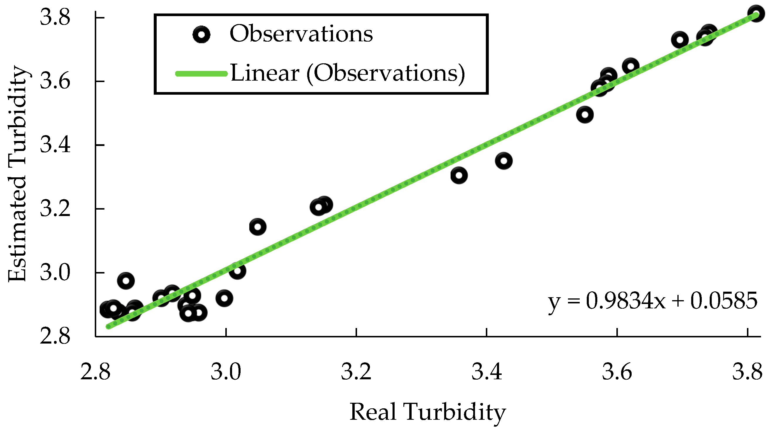
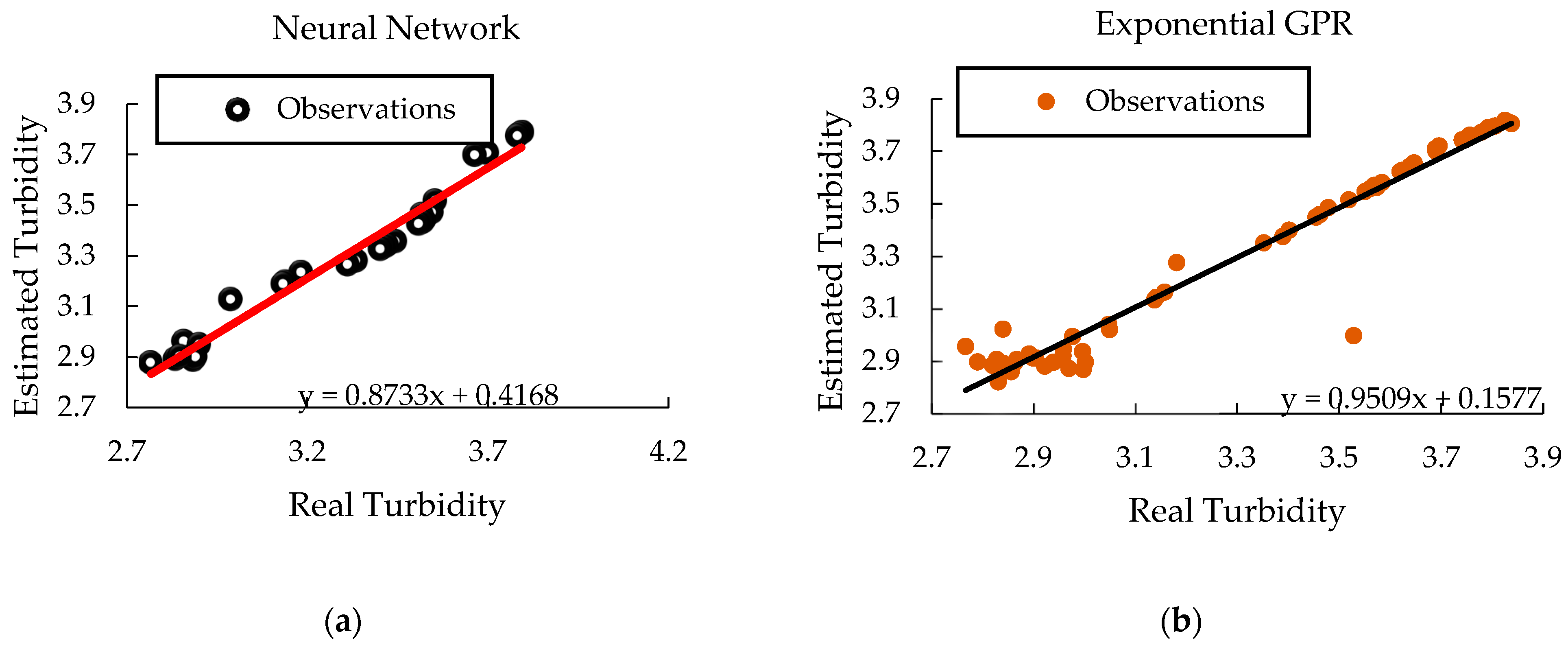
3.4. Mathematical Model Validation

Overfitting can become a prevalent issue while training machine learning models. It happens when a model becomes too complex and starts to fit the training data too closely, resulting in poor generalization performance on new data. Validation is performed to ensure optimal reliability and prevent overfitting of the models that are selected for further analysis. In the current study, validation was conducted on several different models, but the two more relevant models are outlined in

Table 3. Validation metrics of the selected models during training.

Model	R2	MSE	NRSME	AIC
ANN	0.985	0.004	6.01	−160.12
Exponential GPR	0.943	0.008	8.14	−283.02

. The validation results revealed that the exponential GPR model was the least robust for this system, and so the model could not generalize to new data and likely overfitted the training set. It is important to note that the validation process is a crucial step in developing machine learning models. Selecting the most robust model can ensure that results are reliable and can be applied to new data confidently. Overall, the validation process is a vital component of any machine learning workflow and should be given careful consideration when developing new models [54].

Considering the model with the best validation metrics, it can be inferred that ANN represents a forecasting performance with high accuracy (Figure 4). It can be justified because it models complex and nonlinear processes based on a data set using high self-adaptive learning without requiring a normal distribution like conventional methods [55]. Exponential GPR can face challenges in normative modelling due to its assumptions and complexities. These limitations can impact the accuracy and reliability of predictions, especially in scenarios like turbidity prediction, where precise modelling is crucial [56]. While both ANN and GPR have advantages and disadvantages, ANN represents a highly accurate and adaptable approach to complex forecasting tasks. This technology will likely provide valuable insights and predictions that can drive improved decision-making and performance.

Good model reliability is observed when the estimated values are on the diagonal line of the performance graph [57]; the only one that complies, as shown in Figure 4, is the neural network because all the data are scattered close to the solid line. Therefore, it is considered reliable for estimating turbidity in artisanal wines and efficiently represents the estimation of turbidity in artisanal wines. Applying the significance criterion to the selected model, it was found that it is representative with an F of 57.38 and a critical F of 1.44, and so it can be concluded that this model represents the studied system [33]. Even though statistical indicators and error measures indicate that the model obtained in this research can predict wine turbidity, it is highly recommended to continue studying this system so it can be applied to other varieties of grapes or a greater range of variable values, even including more features.

4. Conclusions

The study aimed to determine the best method for measuring wine turbidity using machine learning techniques. According to the Mann–Whitney U test (p-value < 0.05), the ‘yausabara’ fining agent is the most efficient in clarifying Burgundy variety grape wine, as there was a statistical difference between fining agents. Although almost all models trained with MATLAB’s Neural Net Fitting program had a good performance (R² from 0.773 to 0.988, MSE from 0.002 to 0.057, NRSME from 4.9 to 24 and AIC from −387.2 to −814.4), it was found that the Artificial Neural Network (ANN) with 25 neurons and Levenberg–Marquardt algorithm presented not only a good training performance but a good validation performance too (R² of 0.985, MSE of 0.004, NRSME of 6.01 and AIC of −160.12). The SVM model was the only visible method that did not fit the system’s data from those trained with MATLAB’s Regression Learner app. However, among all the other models, the exponential generalized regression prediction (GPR) also yielded good training performance metrics, especially in NRSME and AIC, which have values under 5.5 and −900, respectively.

Furthermore, during the validation of the models, it was discovered that the ANN trained using MATLAB’s Neural Net Fitting technique provided the most accurate representation of the study system, having better validation performance metrics (three of four). This is because the Levenberg–Marquardt algorithm is particularly effective in dealing with smaller networks and is suitable for scenarios where complex relationships must be modelled and learned. The system studied in this research required such complex modelling. Hence, the algorithm was chosen; however, further research is necessary to expand the sampling spectrum and validate the results so the model can be applied to a broader range of wines and the results can be validated more confidently. The results of this research provide a valuable tool for winemakers and researchers and can be used to improve wine quality and consistency.

References

1. Vernhet, A. Red Wine Clarification and Stabilization; Elsevier Inc.: Amsterdam, The Netherlands, 2018; ISBN 9780128144008. [Google Scholar]
2. Carrión Gutiérrez, C.V.; Barrazueta Rojas, S.G.; Mendoza Zurita, G.X.; Lara Freire, M.L. Mejoramiento De Las Propiedades Físicoquímicas Del Vino Usando Distintos Niveles De Bentonita. Cienc. Digit. 2018, 2, 67–87. [Google Scholar] [CrossRef]
3. Dıblan, S.; Özkan, M. Effects of Various Clarification Treatments on Anthocyanins, Color, Phenolics and Antioxidant Activity of Red Grape Juice. Food Chem. 2021, 352, 129321. [Google Scholar] [CrossRef] [PubMed]
4. Mierczynska-Vasilev, A.; Smith, P.A. Current State of Knowledge and Challenges in Wine Clarification. Aust. J. Grape Wine Res. 2015, 21, 615–626. [Google Scholar] [CrossRef]
5. Jones-Moore, H.R.; Jelley, R.E.; Marangon, M.; Fedrizzi, B. The Interactions of Wine Polysaccharides with Aroma Compounds, Tannins, and Proteins, and Their Importance to Winemaking. Food Hydrocoll. 2022, 123, 107150. [Google Scholar] [CrossRef]
6. Li, S.Y.; Duan, C.Q.; Han, Z.H. Grape Polysaccharides: Compositional Changes in Grapes and Wines, Possible Effects on Wine Organoleptic Properties, and Practical Control during Winemaking. Crit. Rev. Food Sci. Nutr. 2023, 63, 1119–1142. [Google Scholar] [CrossRef] [PubMed]
7. Mercurio, M.D.; Dambergs, R.G.; Cozzolino, D.; Herderich, M.J.; Smith, P.A. Relationship between Red Wine Grades and Phenolics. 1. Tannin and Total Phenolics Concentrations. J. Agric. Food Chem. 2010, 58, 12313–12319. [Google Scholar] [CrossRef] [PubMed]
8. Zhai, H.Y.; Li, S.Y.; Zhao, X.; Lan, Y.B.; Zhang, X.K.; Shi, Y.; Duan, C.Q. The Compositional Characteristics, Influencing Factors, Effects on Wine Quality and Relevant Analytical Methods of Wine Polysaccharides: A Review. Food Chem. 2023, 403, 134467. [Google Scholar] [CrossRef] [PubMed]
9. Guilcatoma, B.; Pablo, J.; Sangucho, Y.; Maricela, J.; Castellano, I.T.; Maricela, A.; Latacunga -Ecuador, M. Aplicación de Tres Agentes Clarificantes Yausa (Abutilon insigne p.) Gelatina Y Bentonita Para Clarificar el Vino de Uvilla (Physalis peruviana l.) En el Emprendimiento de la Parroquia de Canchagua. Bachelor’s Thesis, Universidad Técnica de Cotopaxi, Latacunga, Ecuador, 2018. [Google Scholar]
10. Chuma Barrigas, W. Evaluación Del Proceso De Clarificación De Vino De Uva, Artesanal E Industrial, Utilizando Látex De Papaya Papaína Y Gel De ‘Yausabara’ Pavonia Sepium. Bachelor’s Thesis, Universidad Técnica del Norte, Imbabura, Ecuador, 2018. [Google Scholar]
11. Quezada Moreno, W.; Quezada Torres, W.; Gallardo Aguilar, I. Plantas Mucilaginosas En La Clarificación Del Jugo de La Caña de Azúcar. Rev. Cent. Azúcar 2016, 43, 2. [Google Scholar]
12. Al-Risheq, D.I.M.; Shaikh, S.M.R.; Nasser, M.S.; Almomani, F.; Hussein, I.A.; Hassan, M.K. Enhancing the Flocculation of Stable Bentonite Suspension Using Hybrid System of Polyelectrolytes and NADES. Colloids Surf. A Physicochem. Eng. Asp. 2022, 638, 128305. [Google Scholar] [CrossRef]
13. Lukić, I.; Horvat, I.; Radeka, S.; Delač Salopek, D.; Markeš, M.; Ivić, M.; Butorac, A. Wine Proteome after Partial Clarification during Fermentation Reveals Differential Efficiency of Various Bentonite Types. J. Food Compos. Anal. 2024, 126, 305–315. [Google Scholar] [CrossRef]
14. Basha, M.S.A.; Desai, K.; Christina, S.; Sucharitha, M.M.; Maheshwari, A. Enhancing Red Wine Quality Prediction through Machine Learning Approaches with Hyperparameters Optimization Technique. In Proceedings of the 2023 Second International Conference on Electrical, Electronics, Information and Communication Technologies, Trichirappalli, India, 5–7 April 2023; pp. 1–8. [Google Scholar]
15. Fuentes, S.; Torrico, D.D.; Tongson, E.; Viejo, C.G. Machine Learning Modeling of Wine Sensory Profiles and Color of Vertical Vintages of Pinot Noir Based on Chemical Fingerprinting, Weather and Management Data. Sensors 2020, 20, 3618. [Google Scholar] [CrossRef]
16. Cortez, P.; Cerdeira, A.; Almeida, F.; Matos, T.; Reis, J. Modeling Wine Preferences by Data Mining from Physicochemical Properties. Decis. Support Syst. 2009, 47, 547–553. [Google Scholar] [CrossRef]
17. Sun, X.; Wu, B.; Wu, H.; Zhu, H.; Liu, Y. Design of Vineyard Production Monitoring System Based on Wireless Sensor Networks. In Proceedings of the 2011 International Conference on Electronic & Mechanical Engineering and Information Technology, Harbin, China, 12–14 August 2011; Volume 5, pp. 2517–2520. [Google Scholar]
18. Anastasi, G.; Farruggia, O.; Re, G.L.; Ortolani, M. Monitoring High-Quality Wine Production Using Wireless Sensor Networks. In Proceedings of the 2009 42nd Hawaii International Conference on System Sciences, Waikoloa, HI, USA, 5–9 January 2009; pp. 1–7. [Google Scholar] [CrossRef]
19. Pirnau, A.; Feher, I.; Sârbu, C.; Hategan, A.R.; Guyon, F.; Magdas, D.A. Application of Fuzzy Algorithms in Conjunction with 1H-NMR Spectroscopy to Differentiate Alcoholic Beverages. J. Sci. Food Agric. 2023, 103, 1727–1735. [Google Scholar] [CrossRef]
20. Tao, Y.; Wu, D.; Zhang, Q.-A.; Sun, D.-W. Ultrasound-Assisted Extraction of Phenolics from Wine Lees: Modeling, Optimization and Stability of Extracts during Storage. Ultrason. Sonochem. 2014, 21, 706–715. [Google Scholar] [CrossRef]
21. Duarte, D.P.; Oliveira, N.; Georgieva, P.; Nogueira, R.N.; Bilro, L. Wine classification and turbidity measurement by clustering and regression models. In Proceedings of the Conftele 2015: 10th Conference on Telecommunications, Aveiro, Portugal, 17–18 September 2015; pp. 317–320. [Google Scholar]
22. Galeano-Arias, L.F.; Aguirre, S.G.; Castrillón-Gómez, O.D. Wine Quality Analysis through Artificial Intelligence Techniques. Inf. Technol. 2021, 32, 17–26. [Google Scholar] [CrossRef]
23. Jain, K.; Kaushik, K.; Gupta, S.K.; Mahajan, S.; Kadry, S. Machine Learning-Based Predictive Modelling for the Enhancement of Wine Quality. Sci. Rep. 2023, 13, 17042. [Google Scholar] [CrossRef] [PubMed]
24. Mingione, E.; Leone, C.; Almonti, D.; Menna, E.; Baiocco, G.; Ucciardello, N. Artificial Neural Networks Application for Analysis and Control of Grapes Fermentation Process. Procedia CIRP 2022, 112, 22–27. [Google Scholar] [CrossRef]
25. Leza, J.M.I. La Medida de Turbidez Como Elemento Auxiliar de La Filtración. Enoviticultura 2011, 10, 36–41. [Google Scholar]
26. Dahal, K.R.; Dahal, J.N.; Banjade, H.; Gaire, S. Prediction of Wine Quality Using Machine Learning Algorithms. Open J. Stat. 2021, 11, 278–289. [Google Scholar] [CrossRef]
27. Jana, D.K.; Bhunia, P.; Adhikary, S.D.; Mishra, A. Analyzing of Salient Features and Classification of Wine Type Based on Quality through Various Neural Network and Support Vector Machine Classifiers. Results Control Optim. 2023, 11, 100219. [Google Scholar] [CrossRef]
28. Lin, S.; Kim, J.; Hua, C.; Kang, S.; Park, M.H. Comparing Artificial and Deep Neural Network Models for Prediction of Coagulant Amount and Settled Water Turbidity: Lessons Learned from Big Data in Water Treatment Operations. J. Water Process Eng. 2023, 54, 103949. [Google Scholar] [CrossRef]
29. Bazalar, M.; Tejerina, M.; Paganini, J.; Gonzalez, S. Selección de Una Arquitectura de Red Neuronal Artificial Eficiente Para Predecir El Coeficiente de Difusividad Másica Del Aguaymanto (Physalis peruviana L.) Deshidratado Osmoconvectivamente; Universidad Nacional de Trujillo (Perú): Trujillo, Perú, 2013. [Google Scholar]
30. Noor, A.Z.M.; Fauadi, M.H.F.M.; Jafar, F.A.; Bakar, M.H.A. Optimal Number of Hidden Neuron Identification for Sustainable Manufacturing Application. Int. J. Recent Technol. Eng. 2019, 8, 2447–2453. [Google Scholar] [CrossRef]
31. Alcivar-Cevallos, R.; Zambrano-romero, W.D. Predicción Del Rendimiento de Cultivos Agrícolas Usando Aprendizaje Automático. Rev. Arbitr. Interdiscip. Koin. 2020, 5, 144–160. [Google Scholar] [CrossRef]
32. De Porcento, J.; Mendaros, Y.; Moral, R.M.; Cortes, E.P. Enhanced Power Demand Forecasting Accuracy in Heavy Industries Using Regression Learner-Based Approched Machine Learning Model. J. Environ. Energy Sci. 2023, 1, 4–12. [Google Scholar] [CrossRef]
33. Sureiman, O.; Mangera, C. F-Test of Overall Significance in Regression Analysis Simplified. J. Pract. Cardiovasc. Sci. 2020, 6, 116. [Google Scholar] [CrossRef]
34. Quezada, W.; Gallardo, I. Obtención de Extractos de Plantas Mucilaginosas Para La Clarificación de Jugos de Caña Obtainment of Mucilaginous Plant Extrax for Clarification of Cane Juice. Technol. Química 2014, 34, 91–98. [Google Scholar]
35. Ridge, M.; Sommer, S.; Dycus, D.A. Addressing Enzymatic Clarification Challenges of Muscat Grape Juice. Fermentation 2021, 7, 198. [Google Scholar] [CrossRef]
36. Xian, W. Clarifying Effect of Yacon, Pear and Roxburgh Rose Mixture Fermented Fruit Wine. China Brew. 2013, 14, 155. [Google Scholar]
37. Sommer, S.; Tondini, F. Sustainable Replacement Strategies for Bentonite in Wine Using Alternative Protein Fining Agents. Sustainability 2021, 13, 860. [Google Scholar] [CrossRef]
38. Sahin, G.; Işık, G.; van Sark, W. Predictive Modeling of PV Solar Power Plant Efficiency Considering Weather Conditions: A Comparative Analysis of Artificial Neural Networks and Multiple Linear Regression. Energy Rep. 2023, 10, 2837–2849. [Google Scholar] [CrossRef]
39. Incio-Flores, F.A.; Capuñay-Sanchez, D.L.; Estela-Urbina, R.O. Artificial Neural Network Model to Predict Academic Results in Mathematics II. Rev. Electron. Educ. 2023, 27, 1. [Google Scholar] [CrossRef]
40. Gavin, H.P. The Levenberg-Marquardt Algorithm for Nonlinear Least Squares Curve-Fitting Problems; Department of Civil and Environmental Engineering, Duke University: Durham, NC, USA, 2022. [Google Scholar]
41. Rubio, J.D.J. Stability Analysis of the Modified Levenberg-Marquardt Algorithm for the Artificial Neural Network Training. IEEE Trans. Neural Netw. Learn. Syst. 2021, 32, 3510–3524. [Google Scholar] [CrossRef] [PubMed]
42. Li, J. The Application and Modeling of the Levenberg-Marquardt Algorithm. In Proceedings of the 2010 2nd International Conference on E-business and Information System Security, Wuhan, China, 22–23 May 2010. [Google Scholar] [CrossRef]
43. Mammadli, S. Financial Time Series Prediction Using Artificial Neural Network Based on Levenberg-Marquardt Algorithm. Procedia Comput. Sci. 2017, 120, 602–607. [Google Scholar] [CrossRef]
44. Astray, G.; Mejuto, J.C.; Martínez-Martínez, V.; Nevares, I.; Alamo-Sanza, M.; Simal-Gandara, J. Prediction Models to Control Aging Time in Red Wine. Molecules 2019, 24, 826. [Google Scholar] [CrossRef] [PubMed]
45. Hosu, A.; Cristea, V.-M.; Cimpoiu, C. Analysis of Total Phenolic, Flavonoids, Anthocyanins and Tannins Content in Romanian Red Wines: Prediction of Antioxidant Activities and Classification of Wines Using Artificial Neural Networks. Food Chem. 2014, 150, 113–118. [Google Scholar] [CrossRef] [PubMed]
46. Baykal, H.; Yildirim, H.K. Application of Artificial Neural Networks (ANNs) in Wine Technology. Crit. Rev. Food Sci. Nutr. 2013, 53, 415–421. [Google Scholar] [CrossRef] [PubMed]
47. Ye, W.; Melkumian, A.V. Forecasting Australian Red Wine Sales with SARIMA and ANNs. In Proceedings of the 2020 International Symposium on Frontiers of Economics and Management Science (FEMS 2020), Dalian, China, 20–21 March 2020; pp. 140–144. [Google Scholar]
48. Hernández, D.; Espinosa, J.; Peñaloza, M.; Rodriguez, J.; Chacón, J.; Toloza, C.; Arenas, M.; Carrillo, S.; Bermúdez, V. Sobre El Uso Adecuado Del Coeficiente de Correlación de Pearson: Definición, Propiedades y Suposiciones. Rev. Arch. Venez. Farmacol. Ter. 2018, 37, 587–595. [Google Scholar]
49. Cerna Cueva, A.F.; Rosas Echevarría, C.W.; Perales Flores, R.S.; Ataucusi Flores, P.L. Predicción de La Generación de Residuos Sólidos Domiciliarios Con Machine Learning En Una Zona Rural de Puno. Tecnia 2022, 32, 44–52. [Google Scholar] [CrossRef]
50. Sirivanth, P.; Krishna Rao, N.V.; Manduva, J.; Sekhar, G.C.; Tajeswi, M.; Veeresh, C.; Kaushik, J.V. A SVM Based Wine Superiority Estimatation Using Advanced ML Techniques. In Proceedings of the 2021 3rd International Conference on Advances in Computing, Communication Control and Networking (ICAC3N) 2021, Greater Noida, India, 17–18 December 2011; pp. 207–211. [Google Scholar] [CrossRef]
51. Liu, Y. Optimization of Gradient Boosting Model for Wine Quality Evaluation. In Proceedings of the 2021 3rd International Conference on Machine Learning, Big Data and Business Intelligence (MLBDBI), Taiyuan, China, 3–5 December 2021; pp. 128–132. [Google Scholar] [CrossRef]
52. Er, Y.; Atasoy, A. The Classification of White Wine and Red Wine According to Their Physicochemical Qualities. Int. J. Intell. Syst. Appl. Eng. 2016, 4, 23. [Google Scholar] [CrossRef]
53. Patkar, G.S.; Balaganesh, D. Smart Agri Wine: An Artificial Intelligence Approach to Predict Wine Quality. J. Comput. Sci. 2021, 17, 1099–1100. [Google Scholar] [CrossRef]
54. Xu, Y.; Goodacre, R. On Splitting Training and Validation Set: A Comparative Study of Cross-Validation, Bootstrap and Systematic Sampling for Estimating the Generalization Performance of Supervised Learning. J. Anal. Test. 2018, 2, 249–262. [Google Scholar] [CrossRef] [PubMed]
55. Tu, J.; Wei, X.; Huang, B.; Fan, H.; Jian, M.; Li, W. Improvement of Sap Flow Estimation by Including Phenological Index and Time-Lag Effect in Back-Propagation Neural Network Models. Agric. For. Meteorol. 2019, 276–277, 107608. [Google Scholar] [CrossRef]
56. Xu, B.; Kuplicki, R.; Sen, S.; Paulus, M.P. The Pitfalls of Using Gaussian Process Regression for Normative Modeling. PLoS ONE 2021, 16, e0252108. [Google Scholar] [CrossRef] [PubMed]
57. Tchakala, M.; Tafticht, T.; Rahman, M.J. An Efficient Approach for Short-Term Load Forecasting Using the Regression Learner Application. In Proceedings of the 2023 4th International Conference on Clean and Green Energy Engineering (CGEE), Ankara, Turkiye, 26–28 August 2023; pp. 31–34. [Google Scholar]
Figure 1. Fining agent ranges according to the LSD Fisher factor test.
Applsci 14 04416 g001
Figure 2. Performance of the neural network model trained with the Levenberg–Marquardt algorithm with 25 neurons in the hidden layer to predict turbidity in wines.
Applsci 14 04416 g002
Figure 3. Regression Learner performance metrics: (a) coefficient of determination, (b) mean square error, (c) normalized root mean square error, and (d) Aikake information criterion.
Applsci 14 04416 g003
Figure 4. Validation performance of the selected models: (a) neural network and (b) exponential GPR.
Applsci 14 04416 g004