Denoising Multiscale Back-Projection Feature Fusion for Underwater Image Enhancement

Abstract

In recent decades, enhancing underwater images has become a crucial challenge when obtaining high-quality visual information in underwater environment detection, attracting increasing attention. Original underwater images are affected by a variety of underwater environmental factors and exhibit complex degradation phenomena such as low contrast, blurred details, and color distortion. However, most encoder-decoder-based methods fail to restore the details of underwater images due to information loss during downsampling. The noise in images also influences the recovery of underwater images with complex degradation. In order to address these challenges, this paper introduces a simple but effective denoising multiscale back-projection feature fusion network, which represents a novel approach to restoring underwater images with complex degradation. The proposed method incorporates a multiscale back-projection feature fusion mechanism and a denoising block to restore underwater images. Furthermore, we designed a multiple degradation knowledge distillation strategy to extend our method to enhance various types of degraded images, such as snowy images and hazy images. Extensive experiments on the standard datasets demonstrate the superior performance of the proposed method. Qualitative and quantitative analyses validate the effectiveness of the model compared to several state-of-the-art models. The proposed method outperforms previous deep learning models in recovering both the blur and color bias of underwater images.

1. Introduction

In recent years, the processing of underwater images has attracted increasing attention as marine activities increase. Underwater vision plays a crucial role in various applications, including marine biology, underwater archeology, and underwater surveillance. However, underwater vision is still challenging for several reasons. The fog effect produced by suspended particles during the absorption and scattering of light leads to blurred underwater imaging. The difference in the attenuation rate of the light of different wavelengths causes underwater images to show blue shifts or green shifts. The light absorption and scattering in water results in real-world underwater images becoming seriously degraded, causing issues such as color distortion, low contrast, and blurring. The degradation of underwater images severely influences subsequent image-processing tasks, such as automatic object detection and recognition.

As underwater images are similar to low-quality images in the air, early works [1] directly applied traditional image-processing techniques (histogram equalization and gray world) to solve this problem. They usually focus on underwater images with certain kinds of degradation. In addition, these methods easily fail for images with complex degradation. In order to determine the reason for this degradation, many studies [2,3] have analyzed the underwater imaging process and constructed physical models. Therefore, the problem is transformed into an estimation of the parameters of the physical models. However, the accuracy of parameter estimation will largely influence the final performance. In addition, the model cannot adapt to different environments. The traditional methods strongly depend on prior knowledge, which leads to poor results in scenarios where the prior assumptions are not valid.

Recently, deep learning-based underwater image enhancement has become prevalent because of its robustness to different types of underwater images [4,5,6,7]. Compared with traditional underwater image enhancement methods, deep learning-based underwater image enhancement methods do not rely on prior knowledge, have fewer limitations, and achieve better results in most underwater image enhancement. However, several issues remain unsolved. First, most deep learning-based underwater image enhancement methods acquire features at multiple scales [8,9,10,11], and effective fusion mechanisms for multiscale features are lacking. A large amount of detailed information is lost through the encoder-decoder structure due to the downsampling and upsampling processes. On the other hand, many existing methods fail to restore details for underwater images due to noise in the images, especially for complex degradation, such as the combination of color casting and blurring. In order to restore local details in underwater images, an ideal underwater image enhancement method should achieve a balance of color, contrast, and sharpness. Furthermore, the extension of underwater image enhancement methods to handle multiple degradation types remains relatively unexplored. Given the similarity in degradation patterns across various types of images, adapting models to accommodate multiple degradation scenarios is crucial for broader applicability.

In order to address the aforementioned problems and limitations, we propose a denoising multiscale back-projection feature fusion network (DeMBFF-Net) for real-world underwater image enhancement. A multiscale back-projection feature fusion mechanism is introduced for the encoders and decoders. The network can capture both the global context and fine details by processing the feature maps at different scales simultaneously. The back-projection processes iteratively feed the error back during feature fusion, which improves the quality of the recovered images. In order to improve the restoration performance for images with noise, we designed two kinds of denoising blocks for the encoders and decoders. The former focuses on retaining useful information, whereas the latter aims to boost image denoising. In addition, we design a multiple degradation knowledge distillation strategy to extend our method for multitype degradation image enhancement.

The primary contributions of this paper can be summarized as follows:

• Novel denoising back-projection feature fusion mechanism: We present a novel denoising back-projection feature fusion mechanism to effectively integrate multiscale features in underwater image enhancement. This mechanism significantly improves the quality of enhanced images by filtering noise and preserving fine details.
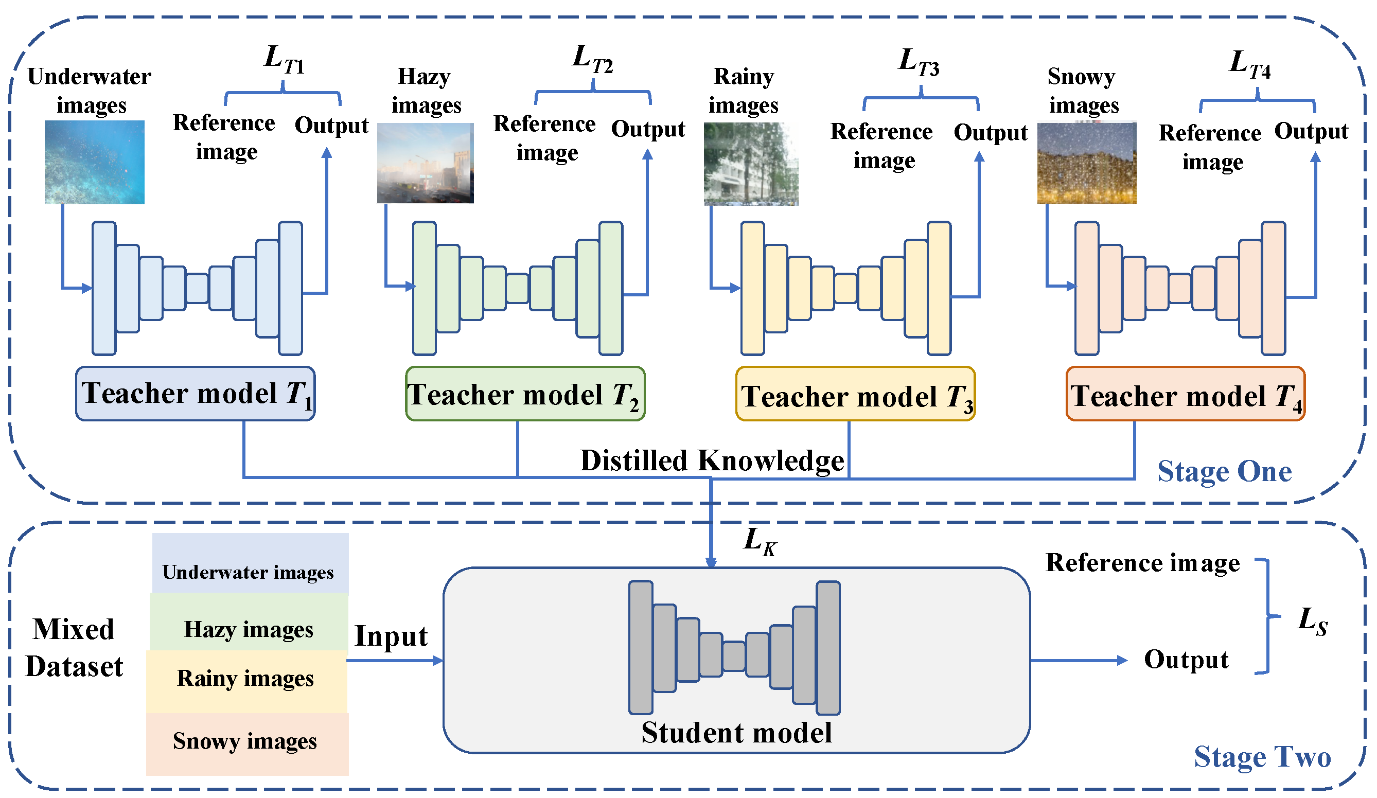
• Multiple degradation knowledge distillation strategy: We introduce a multiple degradation knowledge distillation strategy, enabling our method to generalize across various types of degradation images.
• We evaluate the model on different datasets against other underwater enhancement models. The results indicate that the proposed method achieves the best performance for underwater images with complex degradation. The results of knowledge distillation validate the effectiveness and applicability of our method to address multiple degradation scenarios.

In the following, we first review the related work on underwater image enhancement and then introduce the proposed method in detail. After evaluating the proposed method, we will conclude the work in the final section.

2. Related Work

2.1. Underwater Image Enhancement

Our work is related to single underwater image enhancement. According to the information used, single underwater image enhancement can be divided into three categories: nonmodal-based, modal-based, and data-driven methods.

Nonmodel-based methods: Nonmodel-based methods, such as histogram stretching, histogram equalization, and white balance, directly adjust image pixel values rather than establishing mathematical or physical models. Histogram equalization and its variants are commonly used to enhance the contrast of images. Iqbal et al. [1] improved the contrast and saturation of underwater images by stretching the pixel range in the RGB color space and HSV color space. In addition to low contrast, underwater images also have significant color deviation. As classical image color correction algorithms, the white-balance and gray world methods are widely applied to underwater image enhancement. Ancuti et al. [12] proposed a fusion method that blends a contrast-enhanced image and a color-corrected image at multiple scales. Zhou et al. [13] combined pixel distribution remapping with a multipriority Retinex variational model to address color shift and brightness loss, which efficiently improves image clarity. MCLA [14] utilizes multicolor model conversion and leverages background light and transmission maps, which achieves a good balance between brightness and visibility. Zhou et al. [15] address the nonuniform feature drift problem by using multi-interval subhistogram perspective equalization. This kind of method improves the contrast, brightness, and color of the image but tends to produce undesired artifacts, color cast, or overexposure in the results.

Physical model-based methods: Physical models are usually designed for underwater image restoration to simulate the degradation process of underwater images. By estimating the parameters of the model, the degradation process can be inverted to obtain the normal image. Due to the similarity between underwater imaging models and atmospheric scattering models, many image dehazing algorithms have been applied to underwater image restoration. One of the most influential techniques was dark channel prior (DCP), which was proposed by He et al. [16]. Based on this, Song et al. [17] enhanced underwater images by using a statistical model. Zhou et al. [18] proposed a novel imaging formation model based on a restoration strategy combined with prior knowledge and unsupervised techniques. Since model-based methods assume that underwater images follow a specific physical model, these methods fail when the assumption is not true in the real world.

Data-driven method: With the success of deep learning in many computer vision tasks, it is natural for many researchers to apply these methods to underwater image processing. Early attempts applied deep neural networks to estimate the parameters of physical models, such as background illumination and transmission maps. Therefore, they can be seen as hybrids of physical methods and data-driven methods. The other line of research is to use an end-to-end neural network to achieve enhanced underwater images directly. Deep learning-based underwater image enhancement methods can be classified according to the network structure used, such as CNN-based and GAN-based approaches.

Convolutional neural network-based methods can effectively learn the features of underwater images and remove blurring and color bias from them. In order to better remove blur and color bias from underwater images, UIE-Net [19], which consists of three subnetworks that are responsible for feature extraction, color correction, and defogging, has been used. The gated aggregated convolutional neural network WaterNet [20] feeds the enhanced image obtained via white balance, gamma correction, and histogram equalization to the neural network, together with the original image. Shallow-UWNet [21] is a lightweight CNN network containing only 10 convolutional layers with efficient training and testing speeds and low memory consumption. UWCNN-SD [9] is a two-stage underwater enhancement network that contains a preliminary enhancement network and an improved network. Fu et al. [22] proposed a SCNet underwater image enhancement network based on spatial and channel dimension normalization. SIBM [23] incorporates knowledge of semantic, gradient, and pixel domains to hierarchically enhance underwater images. By considering underwater images in extreme scenarios, ReX-Net [7] leverages the complementary information of reflectance and utilizes attention mechanisms to enhance channel and spatial information. In order to enhance color recovery accuracy, many approaches are used to design different modules, network structures, and strategies. For instance, UGIF-Net [24] proposes a multicolor space-guided color estimation module to adaptively perceive crucial color information during underwater image enhancement. IACC [6] improves color correction by introducing unified luminance features under mixed lighting. MFEF [25] employs white balance and contrast-limited adaptive histogram equalization to introduce multiview features, which provide high-quality and rich features for enhancement.

Since it is difficult to obtain the corresponding clear images for underwater images, the GAN network-based approach can effectively solve the problem of difficult dataset acquisition by using the adversarial learning of generators and discriminators, which does not require pairs of training data and can effectively learn the features of underwater images and clear images. By using CycleGAN, UGAN [26] transforms images from one domain into another without the need for paired training data. WaterGAN [27] uses RGB-D images to simulate underwater images for color correction, and a color correction network is utilized to effectively recover color bias. As a multiscale feature fusion network, MLFcGAN [8] effectively removes the color bias of underwater images. Funie-GAN [28] is a fast, real-time enhancement method that greatly improves the color of images. Recently, HCLR-Net [29] utilizes nonpaired data by introducing a local patch perturbation strategy, developing a more robust sample distribution.

Most existing works explore multiscale information for underwater image enhancement. However, multiscale information is straightforwardly utilized or combined with simple strategies. The information lost during the downsampling and upsampling processes is not utilized effectively. Our method proposes a novel back-projection feature fusion mechanism for multiscale features and introduces denoising blocks in the feature fusion mechanism, which can handle underwater images with complex degradation.

2.2. Back-Projection

Back-projection [30] is an efficient iterative algorithm aimed at minimizing reconstruction errors. It has been widely utilized for super resolutions [31,32,33]. Back-projection learns the difference between high- and low-resolution images in the super-resolution domain to enhance high-resolution images and has been proven to be effective in previous studies. In order to avoid the limitation of predefined parameters, such as blur operators, DBPN [33] uses up-projection and down-projection units, which implement an algorithm with deep learning. Recent work has also validated the fact that the back-projection network can improve the reconstruction of super-resolution video [34].

Inspired by prior works, we propose a denoising multiscale back-projection feature fusion network that utilizes back-projection units to fuse multiscale features during underwater image restoration.

2.3. Knowledge Distillation

Knowledge distillation encompasses a diverse array of techniques aimed at distilling the knowledge contained within a teacher model into a more compact student model [35,36,37]. Hinton et al. [38] introduced the concept of distillation, wherein the student model learns not only from the ground truth labels but also from the softened output probabilities generated by the teacher model. Subsequent works have explored different variants of distillation, including attention-based distillation [39], feature mimicking, and data-free distillation. Recent works have explored techniques such as domain-aware distillation and multitask distillation to improve the transferability and generalization capabilities of distilled models across diverse domains. Multi-teacher distillation is a variant of knowledge distillation that involves distilling knowledge from multiple teacher models into a single student model [40,41,42,43]. In this work, we explore multiteacher distillation for aggregating knowledge from four diverse image enhancements to provide multitask student models with robustness and generalization.

3. Methodology

3.1. Overview

The network proposed in this paper is based on the U-Net architecture with denoising multiscale back-projection feature fusion (DeMBFF) blocks. The network is designed to remove complex degradation, such as blur and color bias, from underwater images, and the specific network structure is shown in Figure 1. The underwater image is input to the encoder. The features are extracted by the encoder using DeMBFF and passed to the next layer of convolution blocks. The last encoder passes all the extracted features into the first decoder. Each decoder receives both the multiscale features from prior layers and the same scale feature from the corresponding encoder via skip connections. All of them are fused by a decoder with DeMBFF, which gradually recovers the clear image. Multiple encoders and decoders with DeMBFF are cascaded to fuse feature maps of different scales from prior layers. The DeMBFF block provides error feedback for feature fusion so that the next layer can better separate the noise information and retain useful information.

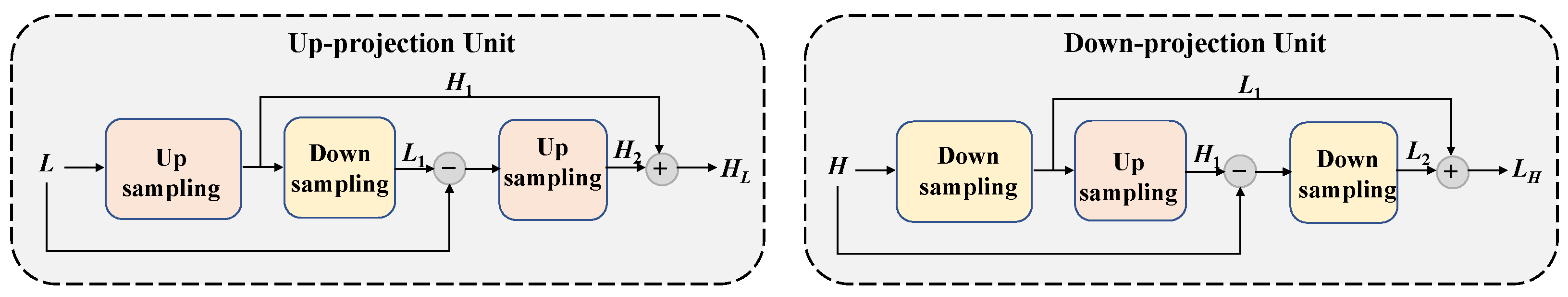
3.2. Revisiting the Back-Projection Algorithm

The back-projection algorithm [30] is a classic algorithm that has wide application for super resolution, medical image processing, and so on. In the field of super resolution (SR), the aim is to recover a high-resolution (HR) image from a low-resolution (LR) image. Unlike deep learning methods, where filters are typically learnable, this algorithm uses a fixed, back-projection kernel for reconstruction. The back-projection algorithm improves image quality by iteratively computing a reconstruction error and integrating it back into the HR image.

For a single, low-resolution image, $I^l$, let the subscripts l and h represent the low-resolution and high-resolution images, respectively, and let t denote the iterative count. The iterative back-projection process can be summarized as follows:

• Initialization: The algorithm initializes the low-resolution image for the first iteration as

  $$I_0^l=I^l.$$

  (1)
• Reconstruction of high-resolution image: At each iteration, a high-resolution image, $I_t^h$, is reconstructed from the previous iteration’s low-resolution image, $I_{t-1}^l$:

  $$I_t^h=(I_{t-1}^l\ast p_t){\uparrow }_s,$$

  (2)

  where $p_t$ is a constant back-projection kernel, differing from deep learning filters that are typically trained. Here, ∗ denotes a spatial convolution operator, and ${\uparrow }_s$ is the upsampling operator with a scaling factor, s.
• Reconstruction error computation: We compute the reconstruction error, $e_r\left(I_t^h\right)$, which is defined as the difference between the low-resolution image and the synthesized high-resolution image of $I_t^h$ by using the following equation:

  $$e_r\left(I_t^h\right)=(I_t^h\ast g_t){\downarrow }_s-I_{t-1}^l,$$

  (3)

  where ${\downarrow }_s$ represents downsampling with scaling factor s. $g_t$ is a blur filter, which is an unlearned predefined parameter.
• Back-projection of error to high-resolution image: The high-resolution image is updated by back-projecting the reconstruction error as follows:

  $$I_t^h\leftarrow I_t^h+(e_r\left(I_t^h\right)\ast p_t){\uparrow }_s,$$

  (4)

  where $p_t$ is the same filter as in Equation (2). The high-resolution image on the right side of this expression is from the reconstruction step in Equation (2). The reconstruction error, $e_r\left(I_t^h\right)$, is from Equation (3).

Since the traditional back-projection process is sensitive to parameter choices, such as the number of iterations, t, filters, $p_t$, and the blur operator, $g_t$, Haris et al. [33] proposed an end-to-end trainable deep back-projection network (DBPN) based on the original algorithm. DBPN consists of up-projection and downprojection units, as shown in Figure 2. The up-projection unit takes the previously computed LR feature map, L, as input and maps it to an HR map, $H_1$. Then, it is mapped back to the LR map (“back-project”). The residual between the observed LR map, L, and the reconstructed map, $L_1$, is mapped to the HR again, which produces a new map: $H_2$. The final output of the up-projection unit, $H_L$, is the sum of the two intermediate HR maps, $H_1$ and $H_2$.

In contrast, the downprojection unit tries to map an HR map, H, to its LR map, $L_H$. The process is similar to that of the up-projection unit. First, the HR map is downsampled to the LR map, and then it is mapped back to the HR map, $H_1$. The difference between the original HR map, H, and the reconstructed HR map, $H_1$, is mapped to obtain another LR map, $L_2$. Finally, the two intermediate LR maps ($L_1$ and $L_2$) are summed together to obtain the output: $L_H$.

DBPN utilizes convolution and deconvolution to implement downsampling and upsampling operations. The outputs of the up-projection and downprojection units are concatenated for the reconstruction of HR images. Unlike the original DBPN, we fuse multiple feature maps from different layers with various scales, which has been proven to be helpful for underwater image enhancement [8,9,10,11]. Inspired by the back-projection algorithm, this paper proposes a multiscale back-projection feature fusion mechanism to restore the missing information of low-scale layers, effectively using the features of nonadjacent layers to improve the blur and color bias while ensuring the sharpness of the image.

3.3. Multiscale Back-Projection Feature Fusion

The encoder of the U-Net structure gradually reduces the size of the feature map during downsampling and expands the perceptual field to better visualize the global information of the feature map. However, the edge information and texture details are lost when all feature maps are transformed to the same scale for fusion. The underwater environment is complex and variable, and the blur and color bias of underwater images are also very uneven in terms of the different depths of objects in the images, which highlights the drawbacks of the U-Net structure. The recovery effect is poor for underwater images with uneven distributions of color bias blur, and information loss leads to a lack of texture details in the restored images.

The multiscale back-projection feature fusion mechanism (MBFF) continuously superimposes multiple scale feature maps to perform scale transformation and feedback errors iteratively. As shown in Figure 3, the input feature is F, and the features of different scales $F_1,\dots ,F_m$ are fused with the input from the back-projection feature fusion block. $F_m$ is the feature map for the scale $S_m$ with $m\in \{1,\dots ,M\}$. The process for one back-projection feature fusion is formally formulated as follows:

For feature $F_m$, the back-projection feature fusion block first upsamples/downsamples the original feature, F, several times until it is the same size as $F_m$. Then, it computes the difference, $e_m$, between the intermediate map, $F_b$, and $F_m$. Then, the downsampling/upsampling process restores the residual map, $e_m$, to its original size. Finally, the back-projecting map is added to the original feature, F, to obtain the fused feature, $F^{\prime }$. The process of fusion feature, $F_m$, using MBFF is illustrated in Algorithm 1. This Algorithm handles situations where $F_m$ has a larger size than F, requiring upsampling followed by downsampling. If $F_m$ is smaller than F, the operations are reversed, with downsampling preceding upsampling.

$$\begin{array}{c}\hfill MBF{F}_{en}(F,F_m)=F+Con\left(Diff(F,Decon\left(F_m\right))\right),\\ \hfill MBF{F}_{de}(F,F_m)=F+Decon\left(Diff(F,Con\left(F_m\right))\right),\end{array}$$

(5)

where $Decon\left(\right)$ is the deconvolution operator used to scale up $F_m$ to the same size as F, and $Con\left(\right)$ denotes the convolution operation that scales down $F_m$ to the same size as F. $Diff(,)$ is the calculation of the residual between F and the scaled $F_m$.

Algorithm 1: Feature fusion process of MBFF for $F_m$.
	Input: Feature F, Fusion feature $F^m$
	Output: The fused feature $F^{\prime }$
1	Calculate deconvolution and convolution times:
2	$Siz{e}_{in}\leftarrow size\left(F\right)$
3	$Siz{e}_{out}\leftarrow size\left(F_m\right)$
4	$times=(Siz{e}_{out}//Siz{e}_{in})//2$
5	Upsampling F with multiple deconvolutions:
6	$F_b\leftarrow Deco{n}_{times}\left(F\right)$
7	Calculate the differences between $F_b$ and $F_m$:
2	$e_m\leftarrow Diff(F_b,F_m)$
9	Down-sampling the differences $e_m$ with multiple convolutions:
10	$e_m\leftarrow Co{n}_{times}\left(e_m\right)$
11	Add the back-projection feature with F:
12	$F^{\prime }=F+e_m$

When taking the fourth encoder, $E{B}^4$, as an example, it merges the output of the features from three separate encoders: $E{B}^1$, $E{B}^2$, and $E{B}^3$. These features are denoted as $F_1$, $F_2$, and $F_3$, with different sizes, as outlined in

Table 1. Specifications of the models used in our method.

	Layer	Input Size	Filter Size	Stride	Activation Function	Output Size
1	Convolution layer	$256\times 256\times 3$	$11\times 11$	1	ReLU	$256\times 256\times 16$
	Convolution layer	$256\times 256\times 16$	$3\times 3$	2	ReLU	$256\times 256\times 16$
2	Convolution layer	$256\times 256\times 16$	$3\times 3$	2	ReLU	$128\times 128\times 32$
	Encoder $E{B}^1$	$128\times 128\times 32$	$3\times 3$	2	ReLU	$128\times 128\times 32$
3	Convolution layer	$128\times 128\times 32$	$3\times 3$	2	ReLU	$64\times 64\times 64$
	Encoder $E{B}^2$	$64\times 64\times 64$	$3\times 3$	2	ReLU	$64\times 64\times 64$
4	Convolution layer	$64\times 64\times 64$	$3\times 3$	2	ReLU	$32\times 32\times 128$
	Encoder $E{B}^3$	$32\times 32\times 128$	$3\times 3$	2	ReLU	$32\times 32\times 128$
5	Convolution layer	$32\times 32\times 128$	$3\times 3$	2	ReLU	$16\times 16\times 256$
	Encoder $E{B}^4$	$16\times 16\times 256$	$3\times 3$	2	ReLU	$16\times 16\times 256$
6	Decoder $D{B}^1$	$16\times 16\times 256$	$3\times 3$	2	ReLU	$16\times 16\times 256$
	Deconvolution layer	$16\times 16\times 256$	$3\times 3$	2	ReLU	$32\times 32\times 128$
7	Decoder $D{B}^2$	$32\times 32\times 128$	$3\times 3$	2	ReLU	$32\times 32\times 128$
	Deconvolution layer	$32\times 32\times 128$	$3\times 3$	2	ReLU	$64\times 64\times 64$
8	Decoder $D{B}^3$	$64\times 64\times 64$	$3\times 3$	2	ReLU	$64\times 64\times 64$
	Deconvolution layer	$64\times 64\times 64$	$3\times 3$	2	ReLU	$128\times 128\times 32$
9	Decoder $D{B}^4$	$128\times 128\times 32$	$3\times 3$	2	ReLU	$128\times 128\times 32$
	Deconvolution layer	$128\times 128\times 32$	$3\times 3$	2	ReLU	$256\times 256\times 16$
10	Convolution layer	$256\times 256\times 16$	$3\times 3$	2	ReLU	$256\times 256\times 16$
	Convolution layer	$256\times 256\times 16$	$3\times 3$	1	ReLU	$256\times 256\times 3$

. They have the size of $256\times 256$ ($F_1$), $128\times 128$ ($F_2$), and $64\times 64$ ($F_3$). The input feature, F, for encoder $E{B}^4$ has a size of $32\times 32\times 128$. In order to fuse with $F^3$, the input feature, F, is upsampled once using deconvolution operations with a filter size of $3\times 3$ and a stride of 2. After upsampling, F has a size of $64\times 64$. Then, the difference between the upsampled F and $F^3$ is computed, resulting in the error feature $e_3$. This error feature, $e_3$, is then downsampled once to reach the original size of F (i.e., $32\times 32\times 128$). The down-sampled $e_3$ is added to the original F, resulting in a new feature: $F^{\prime }$, which represents the output of one back-projection feature fusion block, as shown in Figure 3. In order to fuse with $F^2$, the feature $F^{\prime }$ from the previous step is upsampled twice using convolution operations, achieving a size of $128\times 128$. Similar to the previous step, the error is computed between the upsampled $F^{\prime }$ and $F_2$, and the back-projection process is used to update the feature. The same process is repeated for $F_3$, adjusting the upsampling and downsampling operations accordingly to ensure that the output size matches the input size after each convolution and deconvolution step. This back-projection feature fusion process allows encoder $E{B}^4$ to merge the features from different encoders while maintaining consistent dimensions.

In order to adapt DBPN for multiscale feature fusion, we reduced the number of transformations (upsampling and downsampling operations) from three times to twice. The feature maps from neighboring layers were fused by upsampling or downsampling the current layers using deconvolution or convolution. Omissions can avoid large computational costs for feature fusion. In contrast to DBPNs for super resolution, underwater image enhancement restores images of the same size. Therefore, our network consists of encoders and decoders, which have different structures, as illustrated in Section 3.5 and Section 3.6.

3.4. Denoising Block

Since there is considerable noise that blurs the underwater image, we designed two noise blocks for the encoder and decoder to filter out noise and boost the image, respectively. The denoising blocks for the two stages have similar structures, as shown in Figure 4. Both consist of an attention mechanism, which first calculates the attention weights along the channel axis. Then, the original features are multiplied by the attention coefficient to obtain the features after attention.

$$\begin{array}{c}\hfill Atten\left(F\right)=Mul(F,Con(AvgPool\left(F\right)\left)\right),\end{array}$$

(6)

where $AvgPool\left(\right)$ refers to a pooling operation that reduces the number of channels to 1 while keeping the width and height. $Con\left(\right)$ is the convolution operation, and $Mul(,)$ is the multiplication operation between two inputs. Following attention, the encoder denoising block utilizes two convolution layers and a skip connection to refine the feature further. The mathematical representation of the denoising block in the encoder can be defined as follows:

$$\begin{array}{c}\hfill D{B}_{en}\left(F\right)=Co{n}_{\times 2}\left(Atten\left(F\right)\right)+F.\end{array}$$

(7)

In decoders, the denoising block receives the feature map from the encoder via skip connections. Inspired by the SOS algorithm [44] for boosting image denoising, we first added the feature map of the encoder to that of the decoder, which strengthens the signal. Then, a convolution operation was utilized to denoise the strengthening feature. Finally, we subtracted the previous feature from the restored outcome. The process is formulated as follows:

$$\begin{array}{c}\hfill D{B}_{de}(F,E^{n-K+1})=Diff(Decon\left(Atten\left(F\right)\right),X),\\ \hfill X=Con(Decon\left(Atten\left(F\right)\right)+E^{n-K+1}),\end{array}$$

(8)

where $E^{n-K+1}$ is the feature of the corresponding encoder layers with skip connections. n is the total number of encoders/decoders, and K is the index of the current decoder.

3.5. Encoder with DeMBFF

The encoder design considers two aspects: First, the encoder effectively integrates features from various scales. Second, they need to filter out noise and retain useful information for the restoration. Therefore, we combined the MBFF mechanism (Section 3.3) and the denoising block (Section 3.4) to construct the encoder and decoder, namely, the encoder/decoder with denoising multiscale back-projection feature fusion (DeMBFF). The pseudo-code of the feature fusion process for an encoder with DeMBFF is shown in Algorithm 2.

Algorithm 2: Feature fusion process for encoder with DeMBFF.

For the K-th encoder $E{B}^K$, we denote $E^K$ as the input of the current layer, $E^{K-t}$ as the output feature from the $(K-t)$-th encoder, $FS=\{E^1,\dots ,E^{K-1}\}$ as the multiscale features to be fused in the K-th encoder layer, and $E^K$ represents the features after multiscale back-projection fusion. The feature set, $FS$, consists of the outputs from the 1st to the $K-1$th encoders. The feature fusion calculation for the K-th encoder layer (as shown in Figure 5) is represented as follows:

$$E_t^K=\left\{\begin{array}{cc}D{B}_{en}\left(E^K\right))\hfill & ift=0,\hfill \\ MBF{F}_{en}(E_{t-1}^K,E^{K-t})\hfill & ift>0,\hfill \end{array}\right.$$

(9)

where t indicates the index number of the feature fusion, which ranges from 0 to $K-1$. $D{B}_{en}$ represents the denoising block, and $MBF{F}_{en}$ represents the back-projection feature fusion of the encoder. The multiscale feature fusion mechanism of the encoder is formulated as per Equation (5).

3.6. Decoder with DeMBFF

The decoder with DeMBFF is defined very similarly, but now its task is to upsample and refine features to generate high-quality output. Each encoder consists of several MBFFs from the former layers and one denoising block. In addition, the feature of the encoder is passed via a skip connection. The process is illustrated in Figure 5, which is formulated as follows:

$$D_t^K=\left\{\begin{array}{cc}{D}^K\hfill & ift=0,\hfill \\ MBF{F}_{de}(D_{t-1}^K,D^{K-t})\hfill & if0<t\le K-1,\hfill \\ D{B}_{de}(D_{t-1}^K,E^{n-K+1})\hfill & ift=K,\hfill \end{array}\right.$$

(10)

where $D^K$ represents the input of the current layer, $FS=\{D^1,\dots ,D^{K-1}\}$ represents the multiscale features to be fused in the current decoder, and $D_t^K$ represents the features after multiscale back-projection fusion. $E^{n-K+1}$ indicates the feature of the encoder from the skip connection, where n is the number of encoders. Each decoder fuses features t times, including features from all prior decoders and one corresponding encoder. Therefore, t ranges from 0 to K. The pseudo-code of the feature fusion process for a decoder with DeMBFF is shown in Algorithm 3.

Algorithm 3: Feature fusion process for decoder with DeMBFF.

3.7. Loss Functions

In order to combine both experimental recovery and overhead, the method in this paper uses a mean square error loss function (mean squared error [45]) to calculate the difference between a clear image and an enhanced image. Utilizing the mean squared error loss function in underwater image enhancement tasks helps to remove blur and correct color bias. Specifically, the loss function is calculated as follows:

$$\mathcal{L}(E,G)=\frac{1}{wh}{\parallel E(i,j)-G(i,j)\parallel }^2,$$

(11)

where $(i,j)$ denotes the pixel co-ordinates of the image, and E and G denote the underwater image and the clear image, respectively. $E(i,j)$ and $G(i,j)$ represent the pixel $(i,j)$ in the underwater image, and the co-ordinates are $(i,j)$. w and h denote the width and height of the image, respectively.

4. Multiple Degradation Knowledge Distillation

In order to make the model suitable for multiple types of degradation images, we propose a novel multiple degradation knowledge distillation strategy to implement multitask image enhancement. As illustrated in Figure 6, there are four teacher networks and one student network, where the features of the four teacher models are projected into the student network. The knowledge distillation process includes two stages.

In the first stage, we train four different teacher networks on four kinds of degradation images separately, including underwater images, hazing images, rainy images, and snowy images. The four teacher networks all follow the structure of DeMBFF-Net. For the p-th teacher model $T_p$, we utilize the $L_1$ loss as the loss function, as shown in Equation (12).

$${\mathcal{L}}_{\mathcal{T}}=\frac{1}{wh}\parallel T_p(i,j)-G(i,j)\parallel ,$$

(12)

where $T_p(i,j)$ represents the pixel $(i,j)$ in the restored image by the p-th teacher model, and $G(i,j)$ denotes the same pixel in the clear image. w and h denote the width and height of the image, respectively.

After training the four teacher models, the teachers’ feature maps are distilled to the student network. Following existing work [35], we used the following loss function to make the student’s n-th feature map have similar values to the teacher’s m-th layer.

$${\mathcal{L}}_{\mathcal{K}}=\frac{1}{2}{\parallel T_p^m\left(I\right)-g\left(F^n\left(I\right)\right)\parallel }^2,$$

(13)

where I is the input image. Since we use the same structure for all the teacher and student models, we set m as being equal to n in the above equation. Each teacher transfers an encoder block and a decoder block to the student, resulting in the student network comprising four encoder blocks and four decoder blocks. The convolutional layer g ensures the feature map of the student network keeps the same size as that of the teacher network, which has a kernel size of $3\times 3$ and a stride of 1. In the knowledge distillation setup, the layers in the teacher model are hint layers, and the student layers are guided layers in Equation (13).

After training the guided layers as the initial parameters, we further trained the student network on the mixed dataset (mixed training dataset for four tasks). In the second stage, we designed the following loss function to leverage $L_1$ loss and perception loss.

$${\mathcal{L}}_{\mathcal{S}}=\sum _{i=1}^h\sum _{j=1}^w\parallel S(i,j)-G(i,j)\parallel +\lambda \sum _{i=1}^h\sum _{j=1}^w|{\phi }_{l}S(i,j)-{\phi }_{l}G(i,j)|,$$

(14)

where $\lambda$ is set at $0.5$ to balance the influence of the two different losses. ${\phi }_l$ is the activation of the l-th layer for the VGG network trained on the ImageNet dataset.

5. Experiment and Analysis

In this section, we first introduce the dataset, evaluation metrics, and training details of DeMBFF-Net for the experiment. Next, we perform extensive experiments on three public datasets to investigate the following research problems:

RQ1: How does DeMBFF-Net perform compared to the state-of-the-art and existing methods for subjective evaluation?

RQ2: How does DeMBFF-Net perform compared to the state-of-the-art and existing methods for objective evaluation?

RQ3: How does each design choice made in DeMBFF-Net affect its performance? What is the effect of the DeMBFF block?

RQ4: Can our DeMBFF-Net be used for multiple degradation image enhancement by using the knowledge distillation strategy?

5.1. Datasets

Three underwater image datasets were used to validate the efficiency of our method: the underwater image enhancement benchmark dataset (UIEB) dataset [20], the EUVP dataset [28], and the real-world underwater image enhancement (RUIE) dataset [46]. For testing, the images with inconsistent resolution sizes in the dataset were uniformly cropped to $256\times 256$ pixels.

• The UIEB dataset is an underwater real image dataset with clear images, where the clear images and the enhanced images serve as ground truth. It consists of 950 real-world underwater images, 890 of which have the corresponding clear images.
• The EUVP underwater dataset contains a large collection (20,000) of paired and unpaired underwater images of poor and good perceptual quality. A total of 12,000 of the images have paired clear images, and 8000 of the images have unpaired clear images. The dataset was captured using seven different cameras and contains photos of different visibilities and sea areas.
• The RUIE real underwater dataset comprises 4200 unpaired underwater images captured by moving cameras at different moments in an underwater scene. The images in the dataset exhibit different color shifts and visibility.

In addition, three other kinds of degradation datasets were utilized to evaluate the multiple degradation knowledge distillation process, including the Rain 1400 dataset [47], the RESIDE hazy dataset [48], and the CSD snowy dataset [49].

• The Rain 1400 dataset consists of 1000 pairs of rainy and clear images. The dataset generates 14 rainy images for each clear image, which have different orients.
• The RESIDE hazy dataset is a hazy image dataset with several conditions, which include the training set and the test set. The training data consists of a collection of $13,990$ paired hazy images and clear images. The test set consists of 510 pairs of hazy and clear images.
• The CSD snowy dataset contains 10,000 pairs of snowy images and clear images. The synthetic snowy images simulate snowflakes and snow stripes with different transparencies, sizes, and positions, effectively reflecting real-world snowy scenes.

5.2. Evaluation Metrics

For the testing dataset with reference images, full-reference evaluation was conducted using peak signal-to-noise ratio (PSNR) [50] and structural similarity (SSIM) [51]. Additionally, nonreference evaluation metrics were applied to those datasets lacking ground truth images. We used the underwater image quality measure (UIQM) [52], which is the most widely used no-reference evaluation metric, as the metric. The details about the three metrics are as follows:

• PSNR [50] reflects the proximity to the reference, where a higher PSNR value represents similar image content.
• SSIM [51] represents the degree of similarity of structure and texture for an image pair.
• UIQM [52] consists of three image attribute measurements: underwater image color measurement (UICM), underwater image sharpness measurement (UISM), and underwater image contrast measurement (UIConM). UIQM is a linear combination of these methods, and each property is inspired by the human visual system to assess an aspect of underwater image degradation. A higher value indicates better human visual perception of the color, sharpness, and contrast of the image. The UIQM is calculated as follows:

  $$UIQM=c_1\times UICM+c_2\times UISM+c_3\times UIConM,$$

  (15)

  where $c_1$, $c_2$, and $c_3$ are weighting coefficients. In this paper, we follow the literature [52] and set these as $0.0282$, $0.2953$, and $3.5753$, respectively.

5.3. Experimental Setup

We used Python and PyTorch frameworks via NVIDIA RTX3060 on Windows to implement our method. In the experiment, the batch size was set to 8, and the Adam optimization algorithm [53] was utilized with the following parameters: ${\beta }_1=0.9$ and ${\beta }_2=0.999$. The initial learning rate was set to $0.0001$ and decreased every 50 rounds. Table 1 shows the specifications of the network structure used for experimentation. The input size of the image was $256\times 256$.

5.4. Training Process

For the underwater image enhancement task, the UIEB and EUVP datasets were randomly divided into 10 equal folds. During the training process, nine of these folds were randomly selected for training, with the remaining one used for testing. This process was repeated several times on the two datasets to compute the average values for the final results. Since the RUIE dataset only contains underwater images without corresponding clear images, we used the model trained on UIEB to enhance the images in the following results.

For the multiple-type image enhancement task, we utilized the UIEB, RESIDE, Rain 1400, and CSD datasets for training and testing. Since these datasets contain varying numbers of images, we randomly selected 800 images from each dataset to ensure a balanced set. These subsets were denoted as $Dat{a}_{UIEB}$, $Dat{a}_{RESIDE}$, $Dat{a}_{Rain}$, and $Dat{a}_{CSD}$. Each of these four subsets was split into training and testing sets, with $80\%$ used for training and the remaining $20\%$ for testing. Initially, each subset was used to train a different teacher model. After training the teacher models, the training datasets were mixed together to serve as training data for the student model. The testing datasets were used to evaluate the performance of the student model.

5.5. Comparative Methods

In order to verify the effectiveness of the method proposed in this paper, we compared it with two classical methods based on physical models and six recent methods based on neural networks. The methods for comparison include DCP [16], UDCP [54], DeepSesr [10], Funie-GAN [28], MLFcGAN [8], UWCNN-SD [9], SUSIR [55], and SCNET [22].

We also conducted experiments on multiple low-quality image datasets, comparing these with existing classical and state-of-the-art deep learning-based methods. For the dehazing task, the comparative methods included PFDN [56], FFA-Net [57], AECR-Net [58], D4 [59], and All-in-one [60]. For the rainy dataset, the comparative methods included PreNet [61], MSPFN [62], DualGCN [63], JRGR [64], and All-in-one [60]. For the desnow task, the comparative methods included DesnowNet [65], JSTASR [66], HDCW-Net [49], and All-in-one [60].

5.6. Qualitative Analysis

For the visual comparisons, we first selected several underwater images from the UIEB, EUVP, and RUIE datasets, which consist of three categories: greenish images, bluish images, and turbid images. The results of the different methods and the corresponding reference images (ground truth) are shown in Figure 7, Figure 8 and Figure 9.

Visual comparisons on the UIEB dataset: Figure 7 presents the enhancement results of the proposed method and other methods on the UIEB underwater dataset for various test images. Traditional methods based on physical models, such as DCP and UDCP, show limited effectiveness in correcting blue-green color bias. Several methods (DeepSear, Funie-GAN, and MLFcGAN) tend to produce red casts in turbid images. The proposed method effectively removes both blur and image color bias, resulting in clear texture details, sharp edge colors, and high contrast. The produced image is closest to the original clear image for all three kinds of underwater images (greenish images, bluish images, and turbid images).

Visual comparisons on the EUVP dataset: Figure 8 shows the enhancement results on the EUVP underwater dataset. Most images in the EUVP dataset are greenish or bluish. Traditional methods, such as DCP and UDCP, exhibit less effectiveness in correcting color bias, while newer methods, such as DeepSesr, Funie-GAN, MLFcGAN, and SCNET, achieve relatively better results. However, most of the methods fail to restore those images with heavy color casts (the third and sixth rows in Figure 8). The proposed DeMBFF-Net outperforms the others by effectively removing blurring and color bias, resulting in clear textural details. The overall color recovery is closest to that of the original clear image.

Visual comparisons on the RUIE dataset: Figure 9 illustrates the enhancement results on the RUIE real underwater dataset. Traditional methods, such as DCP and UDCP, show poor image recovery. For underwater images with only mild blue color bias (the first and second rows), the depth-based methods achieve better results. For underwater images with only green color bias (the third and fourth rows in Figure 9), only the UWCNN-SD and our method effectively remove the color bias. For underwater images with both slight color bias and blur (the fifth and sixth rows), only the SCNET and DeMBFF-Net methods remove both blur and color bias. The results show that our method has higher contrast, better clarity, and better subjective effects than the other methods.

5.7. Quantitative Evaluation

The comparison results between the method proposed in this paper and the above methods on the UIEB, EUVP, and RUIE datasets are listed in

Table 2. Quantitative comparison among different methods on the UIEB dataset. The highest PSNR, SSIM, UIQM, UICM, UISM and UIConM scores are marked in bold text.

Metric	DCP	UDCP	DeepSesr	Funie-GAN	MLFCGAN	UWCNN-SD	USUIR	SCNET	Ours
PSNR↑	$20.1146$	$17.8654$	$22.8564$	$23.1245$	$22.8165$	$22.9035$	$24.6758$	$25.1093$	$\mathbf{26}.\mathbf{4521}$
SSIM↑	$0.7545$	$0.7061$	$0.8631$	$0.8786$	$0.8629$	$0.8247$	$0.8927$	$0.9114$	$\mathbf{0}.\mathbf{9286}$
UIQM↑	$2.223\pm 0.600$	$2.076\pm 0.497$	$3.032\pm 0.363$	$3.023\pm 0.284$	$2.929\pm 0.353$	$2.936\pm 0.242$	$3.039\pm 0.299$	$3.123\pm 0.242$	$\mathbf{3}.\mathbf{141}\pm \mathbf{0}.\mathbf{274}$
UICM↑	$6.186\pm 3.302$	$7.392\pm 3.310$	$5.343\pm 3.309$	$\mathbf{7}.\mathbf{510}\pm \mathbf{3}.\mathbf{068}$	$4.911\pm 3.130$	$5.830\pm 2.490$	$6.666\pm 2.956$	$6.676\pm 2.836$	$5.436\pm 3.211$
UISM↑	$5.644\pm 1.259$	$5.657\pm 1.271$	$6.502\pm 1.194$	$6.719\pm 0.773$	$6.231\pm 1.080$	$6.333\pm 0.730$	$6.422\pm 0.974$	$6.692\pm 0.983$	$\mathbf{6}.\mathbf{851}\pm \mathbf{0}.\mathbf{598}$
UIConM ↑	$0.107\pm 0.084$	$0.055\pm 0.054$	$0.269\pm 0.053$	$0.231\pm 0.058$	$0.266\pm 0.050$	$0.252\pm 0.032$	$0.267\pm 0.048$	$0.268\pm 0.036$	$\mathbf{0}.\mathbf{270}\pm \mathbf{0}.\mathbf{051}$

,

Table 3. Quantitative comparison among different methods on the EUVP dataset. The highest PSNR, SSIM, UIQM, UICM, UISM and UIConM scores are marked in bold text.

Metric	DCP	UDCP	DeepSesr	Funie-GAN	MLFCGAN	UWCNN-SD	USUIR	SCNET	Ours
PSNR↑	$18.5168$	$17.0162$	$22.4644$	$23.6628$	$23.3562$	$21.1916$	$22.0390$	$24.1001$	$\mathbf{26}.\mathbf{1282}$
SSIM↑	$0.6466$	$0.5561$	$0.8062$	$0.8264$	$0.8108$	$0.7838$	$0.8085$	$0.8303$	$\mathbf{0}.\mathbf{8816}$
UIQM↑	$2.042\pm 0.471$	$1.981\pm 0.444$	$3.051\pm 0.358$	$2.977\pm 0.309$	$2.864\pm 0.356$	$2.980\pm 0.164$	$2.984\pm 0.257$	$3.001\pm 0.289$	$\mathbf{3}.\mathbf{097}\pm \mathbf{0}.\mathbf{268}$
UICM↑	$4.881\pm 2.615$	$\mathbf{5}.\mathbf{557}\pm \mathbf{1}.\mathbf{158}$	$4.648\pm 2.592$	$4.641\pm 2.759$	$4.097\pm 2.243$	$4.826\pm 2.229$	$7.123\pm 2.336$	$5.669\pm 2.143$	$4.558\pm 2.314$
UISM↑	$5.458\pm 1.08$	$5.557\pm 1.158$	$6.557\pm 1.18$	$6.474\pm 0.781$	$6.080\pm 0.981$	$6.404\pm 0.598$	$6.107\pm 0.941$	$6.330\pm 0.981$	$\mathbf{6}.\mathbf{712}\pm \mathbf{0}.\mathbf{883}$
UIConM↑	$0.082\pm 0.065$	$0.044\pm 0.044$	$0.275\pm 0.048$	$0.261\pm 0.058$	$0.267\pm 0.06$	$0.267\pm 0.033$	$0.274\pm 0.038$	$0.272\pm 0.046$	$\mathbf{0}.\mathbf{276}\pm \mathbf{0}.\mathbf{056}$

and

Table 4. Quantitative comparison among different methods on the RUIE dataset. The highest UIQM, UICM, UISM and UIConM scores are marked in bold text.

Metric	DCP	UDCP	DeepSesr	Funie-GAN	MLFCGAN	UWCNN-SD	USUIR	SCNET	Ours
UIQM↑	$2.254\pm 0.415$	$2.311\pm 0.296$	$3.113\pm 0.254$	$3.090\pm 0.235$	$2.952\pm 0.206$	$3.189\pm 0.102$	$3.133\pm 0.116$	$3.169\pm 0.132$	$\mathbf{3}.\mathbf{210}\pm \mathbf{0}.\mathbf{230}$
UICM↑	$2.29\pm 1.583$	$5.101\pm 2.38$	$\mathbf{6}.\mathbf{228}\pm \mathbf{1}.\mathbf{024}$	$3.235\pm 1.72$	$2.351\pm 1.046$	$2.355\pm 0.775$	$5.275\pm 1.751$	$3.325\pm 1.084$	$2.585\pm 1.071$
UISM↑	$6.14\pm 0.813$	$6.517\pm 0.558$	$6.763\pm 0.576$	$6.666\pm 0.691$	$6.170\pm 0.603$	$7.062\pm 0.308$	$6.676\pm 0.527$	$6.759\pm 0.567$	$\mathbf{6}.\mathbf{817}\pm \mathbf{0}.\mathbf{883}$
UIConM↑	$0.105\pm 0.054$	$0.068\pm 0.052$	$0.263\pm 0.041$	$0.288\pm 0.046$	$0.298\pm 0.042$	$0.290\pm 0.022$	$0.283\pm 0.025$	$0.302\pm 0.031$	$\mathbf{0}.\mathbf{314}\pm \mathbf{0}.\mathbf{043}$

. These values represent the average results over five trials.

Full-Reference Evaluation: The UIEB and EUVP datasets were used for this evaluation. The statistical results and visual comparisons are summarized in Table 2 and Table 3. As the two tables show, our DeMBFF-Net demonstrates the best performance for both the PSNR and SSIM metrics. Specifically, our method outperforms other methods in terms of image quality and recovery. It also illustrates that our method achieves the highest values for all the indicators except for UICM, indicating exceptional recovery effects in terms of sharpness and contrast. The overall effect of the recovered image is closer to that of the real image according to the following subjective results.

Nonreference Evaluation: The UIEB, EUVP, and RUIE datasets were used for the nonreference evaluation, in which the statistical results are represented in Table 2, Table 3 and Table 4. The results for the RUIE dataset were obtained using the model trained on the UIEBD dataset. Visual comparisons are shown in Figure 7, Figure 8 and Figure 9. Our method achieved the highest score for the UIQM metrics for these three datasets, which confirmed its ability to generalize to various real-world underwater scenes. For the three items of the UIQM, our method has the highest values for UISM and UIConM, indicating exceptional recovery effects in terms of sharpness and contrast. The following visual comparison results are consistent with the objective results.

5.8. Ablation Experiments

In order to assess the impact of the DeMBFF mechanism proposed in this paper, ablation experiments were conducted on the UIEB dataset. Four variations of the model were evaluated:

• w/o DeMBFF: A base U-Net model without an MBFF or denoising block, which includes a simple encoder, decoder, and jump connections;
• With a DB: A base U-Net model with a denoising block (DB) in the encoder and decoder;
• With MBFF: A base U-Net model with MBFF and without a DB in the encoder and decoder;
• With DeMBFF: The full model that includes encoders and decoders with the DeMBFF mechanism.

The results of the ablation experiments are presented in

Table 5. Results of ablation experiments on the UIEB dataset. The × and ✓ notations indicate the presence and absence of each component, respectively. Bold text denotes the highest value for each measurement.

Dataset	Ablation	Denosing Block	MBFF	PSNR	SSIM	UIQM
UIEB	w/o DeMBFF	×	×	$22.7648$	$0.8706$	$3.031\pm 0.311$
	with DB	✓	×	$24.5812$	$0.8535$	$3.042\pm 0.302$
	with MBFF	×	✓	$24.9138$	$0.8598$	$3.078\pm 0.323$
	with DeMBFF	✓	✓	$\mathbf{26.4521}$	$\mathbf{0.9286}$	$\mathbf{3.141}\pm \mathbf{0.274}$

. The addition of a DB and MBFF to the base model improves the PSNR, SSIM, and UIQM. The combination of DeMBFF achieves a significant improvement compared to the other three models, highlighting the effectiveness of DeMBFF in enhancing the quality of underwater image restoration.

As shown in Figure 10, the results confirm that the DdMBFF mechanism can significantly reduce color bias and blurring in underwater images. It is obvious that the original underwater image in the first column contains multiple degradation phenomena: both color bias and blurring problems. The base network model with DB, shown in the third column, can somewhat reduce the blurring problem. However, some areas still lack detailed restoration (as indicated by the red box). In contrast, the model with MBFF (the fourth column) promotes the details when compared to the model with DB. The full model (with DeMBFF) has a balance between color bias and sharpness in the underwater images and effectively restores the details. The results validate that our approach maintains the most valuable information for enhancement through feature fusion.

In order to assess the impact of the number of encoder/decoder layers on the performance of DeMBFF-Net, we varied the number of layers from 2 to 5. As the number of layers increases, both the computational load for feature fusion and the number of parameters increase. The results of this investigation are presented in

Table 6. Results of different numbers of layers on the UIEB dataset. Bold text denotes the highest value for each measurement.

Encoder/Decoder Number	Params (M)	PSNR	SSIM	UIQM	UICM	UISM	UIConM
2	1.99	$22.3418$	$0.8942$	$3.064\pm 0.25$	$7.304\pm 3.154$	$6.86\pm 0.649$	$0.233\pm 0.058$
3	8.35	$23.2525$	$0.9048$	$3.046\pm 0.295$	$7.182\pm 3.129$	$6.791\pm 0.764$	$0.234\pm 0.06$
4	31.35	$\mathbf{26.4521}$	$\mathbf{0.9286}$	$\mathbf{3.141}\pm \mathbf{0.274}$	$5.436\pm 3.211$	$\mathbf{6.851}\pm \mathbf{0.598}$	$\mathbf{0.270}\pm \mathbf{0.051}$
5	131.07	$23.6035$	$0.9137$	$3.052\pm 0.275$	$\mathbf{7.416}\pm \mathbf{3.04}$	$6.747\pm 0.821$	$0.238\pm 0.05$

. Specifically, the parameter count rose from 31.35 M to 131.07 M when the number of layers increased from 4 to 5. This significant increase indicates a considerable rise in computational overhead with additional layers. At the same time, the performance dropped as the layer increased, possibly due to overfitting on the training dataset. In order to find an optimal balance between performance and efficiency, we chose to set the number of encoder/decoder layers to 4 for our experiments. This configuration offers a trade-off that ensures reasonable computational demands while maintaining acceptable performance levels.

5.9. Results for Multi-Type Degradation Image Enhancement

After applying the student model after knowledge distillation to enhance the three different types of degraded images, namely, rainy, snowy, and hazy images, we conducted a thorough visual performance evaluation to assess the qualitative improvement achieved. Figure 11 illustrates the restored results for three types of images, including rainy images (top left), snowy images (bottom left), and hazy images (right). The four teacher models were first trained on four datasets separately. Then, the student model was retrained on the mixed dataset (detailed in Section 5.4).

For the rainy images, our method effectively reduced the noise and enhanced image clarity. The restored images exhibit a noticeable reduction in rain streaks and distortion, resulting in clearer and more defined objects and scenes. Fine details, such as textures and edges, were better preserved, leading to visually pleasing enhancements.

Similarly, for the snowy images, our method successfully mitigated the adverse effects of snow accumulation. The enhanced images exhibit smoother surfaces, with reduced snow artifacts and improved visibility of the underlying details. The snow-covered regions were effectively cleared, revealing clearer and sharper image content.

Furthermore, for the hazy images, our method significantly improved visibility and contrast. The restored images displayed enhanced clarity and color vibrancy, with reduced haze and improved overall visibility of distant objects. The fine details obscured by haze were recovered, resulting in crisper and more visually appealing images.

Overall, the visual performance evaluation demonstrates the effectiveness and generalization of our proposed process in enhancing various types of degraded images. The qualitative improvements observed in the restored images highlight the capability of our method to restore image clarity, reduce artifacts, and enhance overall visual quality across different environmental conditions.

6. Conclusions

In this study, we introduce a denoising multiscale back-projection feature fusion network designed to address multiscale feature fusion and complex degradation. Our core module, DeMBFF, introduces the back-projection algorithm and denoising block into multiscale feature fusion for underwater image enhancement. By leveraging multiscale back-projection feature fusion, the network iteratively feeds errors back for image enhancement. The combination of denoising blocks enables DeMBFF to enhance deblurring performance. The multiple degradation knowledge distillation strategy adapts the model to accommodate multiple degradation scenarios. Through qualitative and quantitative experiments on standard datasets, the results demonstrate that DeMBFF-Net performs well across various datasets and significantly improves image color and clarity. In particular, it excels in addressing underwater images with complex degradation, which achieves a balance between color correction and deblurring for underwater images. In the future, we will seek to improve the model’s performance for images with low illumination and enhance color consistency and brightness for heavily degraded images.

References

1. Kashif, I.; Michael, O.; Anne, J.; Rosalina, S.A.; Hj, T.A.Z. Enhancing the low quality images using Unsupervised Colour Correction Method. In Proceedings of the IEEE International Conference on Systems, Man and Cybernetics, Istanbul, Turkey, 10–13 October 2010. [Google Scholar]
2. Chiang, J.Y.; Chen, Y.C. Underwater Image Enhancement by Wavelength Compensation and Dehazing. IEEE Trans. Image Process. 2012, 21, 1756–1769. [Google Scholar] [CrossRef] [PubMed]
3. Akkaynak, D.; Trebitz, T. Sea-Thru: A Method For Removing Water From Underwater Images. In Proceedings of the IEEE Computer Society Conference on Computer Vision and Pattern Recognition, Long Beach, CA, USA, 15–20 June 2019. [Google Scholar]
4. Li, C.; Anwar, S.; Porikli, F. Underwater scene prior inspired deep underwater image and video enhancement. Pattern Recognit. 2020, 98, 107038. [Google Scholar] [CrossRef]
5. Pritish, U.; Wu, Z.; Wang, Z. All-in-One Underwater Image Enhancement Using Domain-Adversarial Learning. In Proceedings of the IEEE Conference on Computer Vision and Pattern Recognition Workshops, Long Beach, CA, USA, 15–20 June 2019. [Google Scholar]
6. Zhou, J.; Gai, Q.; Zhang, D.; Lam, K.; Zhang, W.; Fu, X. IACC: Cross-Illumination Awareness and Color Correction for Underwater Images Under Mixed Natural and Artificial Lighting. IEEE Trans. Geosci. Remote. Sens. 2024, 62, 1–15. [Google Scholar] [CrossRef]
7. Zhang, D.; Zhou, J.; Zhang, W.; Lin, Z.; Yao, J.; Polat, K.; Alenezi, F.; Alhudhaif, A. ReX-Net: A reflectance-guided underwater image enhancement network for extreme scenarios. Expert Syst. Appl. 2023, 231, 120842. [Google Scholar] [CrossRef]
8. Liu, X.; Gao, Z.; Chen, B.M. MLFcGAN: Multilevel Feature Fusion-Based Conditional GAN for Underwater Image Color Correction. IEEE Geosci. Remote Sens. Lett. 2020, 17, 1488–1492. [Google Scholar] [CrossRef]
9. Wu, S.; Luo, T.; Jiang, G.; Yu, M.; Xu, H.; Zhu, Z.; Song, Y. A Two-Stage Underwater Enhancement Network Based on Structure Decomposition and Characteristics of Underwater Imaging. IEEE J. Ocean. Eng. 2021, 46, 1213–1227. [Google Scholar] [CrossRef]
10. Islam, M.J.; Luo, P.; Sattar, J. Simultaneous Enhancement and Super-Resolution of Underwater Imagery for Improved Visual Perception. In Proceedings of the Robotics: Science and Systems XVI, Virtual Event, Corvalis, OR, USA, 12–16 July 2020. [Google Scholar]
11. Zhou, J.; Zhang, D.; Zhang, W. Cross-view enhancement network for underwater images. Eng. Appl. Artif. Intell. 2023, 121, 105952. [Google Scholar] [CrossRef]
12. Ancuti, C.; Ancuti, C.O.; Haber, T.; Bekaert, P. Enhancing underwater images and videos by fusion. In Proceedings of the IEEE Conference on Computer Vision and Pattern Recognition, Providence, RI, USA, 16–21 June 2012. [Google Scholar]
13. Zhou, J.; Wang, S.; Lin, Z.; Jiang, Q.; Sohel, F. A Pixel Distribution Remapping and Multi-prior Retinex Variational Model for Underwater Image Enhancement. IEEE Trans. Multimed. 2024, 99, 1–12. [Google Scholar] [CrossRef]
14. Zhou, J.; Wang, Y.; Li, C.; Zhang, W. Multicolor Light Attenuation Modeling for Underwater Image Restoration. IEEE J. Ocean. Eng. 2023, 48, 1322–1337. [Google Scholar] [CrossRef]
15. Zhou, J.; Pang, L.; Zhang, D.; Zhang, W. Underwater Image Enhancement Method via Multi-Interval Subhistogram Perspective Equalization. IEEE J. Ocean. Eng. 2023, 48, 474–488. [Google Scholar] [CrossRef]
16. He, K.; Sun, J.; Tang, X. Single Image Haze Removal Using Dark Channel Prior. IEEE Trans. Pattern Anal. Mach. Intell. 2011, 33, 2341–2353. [Google Scholar]
17. Song, W.; Wang, Y.; Huang, D.; Liotta, A.; Perra, C. Enhancement of Underwater Images With Statistical Model of Background Light and Optimization of Transmission Map. IEEE Trans. Broadcast. 2020, 66, 153–169. [Google Scholar] [CrossRef]
18. Zhou, J.; Liu, Q.; Jiang, Q.; Ren, W.; Lam, K.M.; Zhang, W. Underwater camera: Improving visual perception via adaptive dark pixel prior and color correction. Int. J. Comput. Vis. 2023. [Google Scholar] [CrossRef]
19. Wang, Y.; Zhang, J.; Cao, Y.; Wang, Z. A deep CNN method for underwater image enhancement. In Proceedings of the IEEE International Conference on Image Processing, Beijing, China, 17–20 September 2017; pp. 1382–1386. [Google Scholar]
20. Li, C.; Guo, C.; Ren, W.; Cong, R.; Hou, J.; Kwong, S.; Tao, D. An Underwater Image Enhancement Benchmark Dataset and Beyond. IEEE Trans. Image Process. 2020, 29, 4376–4389. [Google Scholar] [CrossRef]
21. Naik, A.; Swarnakar, A.; Mittal, K. Shallow-UWnet: Compressed Model for Underwater Image Enhancement (Student Abstract). In Proceedings of the Thirty-Fifth AAAI Conference on Artificial Intelligence, AAAI 2021, Virtual Event, 2–9 February 2021; pp. 15853–15854. [Google Scholar]
22. Fu, Z.; Lin, X.; Wang, W.; Huang, Y.; Ding, X. Underwater Image Enhancement Via Learning Water Type Desensitized Representations. In Proceedings of the ICASSP 2022, Virtual and Singapore, 23–27 May 2022; pp. 2764–2768. [Google Scholar]
23. Mu, P.; Qian, H.; Bai, C. Structure-Inferred Bi-level Model for Underwater Image Enhancement. In Proceedings of the MM ’22: The 30th ACM International Conference on Multimedia, Lisboa, Portugal, 10–14 October 2022; pp. 2286–2295. [Google Scholar]
24. Zhou, J.; Li, B.; Zhang, D.; Yuan, J.; Zhang, W.; Cai, Z.; Shi, J. UGIF-Net: An Efficient Fully Guided Information Flow Network for Underwater Image Enhancement. IEEE Trans. Geosci. Remote Sens. 2023, 61, 1–17. [Google Scholar] [CrossRef]
25. Zhou, J.; Sun, J.; Zhang, W.; Lin, Z. Multi-view underwater image enhancement method via embedded fusion mechanism. Eng. Appl. Artif. Intell. 2023, 121, 105946. [Google Scholar] [CrossRef]
26. Fabbri, C.; lslam, M.J.; Sattar, J. Enhancing underwater imagery using generative adversarial networks. In Proceedings of the IEEE International Conference on Robotics and Automation, Brisbane, Australia, 21–25 May 2018. [Google Scholar]
27. Li, J.; Katherine, S.; M.Eustice, R.; Johnson-Roberson, M. WaterGAN: Unsupervised generative network to enable real-time color correction of monocular underwater images. IEEE Robot. Autom. Lett. 2018, 3, 387–394. [Google Scholar] [CrossRef]
28. Islam, M.J.; Xia, Y.; Sattar, J. Fast Underwater Image Enhancement for Improved Visual Perception. IEEE Robot. Autom. Lett. 2020, 5, 3227–3234. [Google Scholar] [CrossRef]
29. Zhou, J.; Sun, J.; Li, C.; Jiang, Q.; Zhou, M.; Lam, K.M.; Zhang, W.; Fu, X. HCLR-Net: Hybrid Contrastive Learning Regularization with Locally Randomized Perturbation for Underwater Image Enhancement. Int. J. Comput. Vis. 2024. [Google Scholar] [CrossRef]
30. Irani, M.; Peleg, S. Motion Analysis for Image Enhancement: Resolution, Occlusion, and Transparency. J. Vis. Commun. Image Represent. 1993, 4, 324–335. [Google Scholar] [CrossRef]
31. Dai, S.; Han, M.; Wu, Y.; Gong, Y. Bilateral Back-Projection for Single Image Super Resolution. In Proceedings of the 2007 IEEE International Conference on Multimedia and Expo, ICME 2007, IEEE Computer Society, Beijing, China, 2–5 July 2007; pp. 1039–1042. [Google Scholar]
32. Zhao, Y.; Wang, R.; Jia, W.; Wang, W.; Gao, W. Iterative projection reconstruction for fast and efficient image upsampling. Neurocomputing 2017, 226, 200–211. [Google Scholar] [CrossRef]
33. Haris, M.; Shakhnarovich, G.; Ukita, N. Deep Back-Projection Networks for Single Image Super-Resolution. IEEE Trans. Pattern Anal. Mach. Intell. 2021, 43, 4323–4337. [Google Scholar] [CrossRef] [PubMed]
34. Luo, C.; Li, B.; Liu, F. Iterative Back Projection Network Based on Deformable 3D Convolution. IEEE Access 2023, 11, 122586–122597. [Google Scholar] [CrossRef]
35. Gou, J.; Yu, B.; Maybank, S.J.; Tao, D. Knowledge Distillation: A Survey. Int. J. Comput. Vis. 2021, 129, 1789–1819. [Google Scholar] [CrossRef]
36. Wang, L.; Yoon, K. Knowledge Distillation and Student-Teacher Learning for Visual Intelligence: A Review and New Outlooks. IEEE Trans. Pattern Anal. Mach. Intell. 2022, 44, 3048–3068. [Google Scholar] [CrossRef] [PubMed]
37. Li, Z.; Xu, P.; Chang, X.; Yang, L.; Zhang, Y.; Yao, L.; Chen, X. When Object Detection Meets Knowledge Distillation: A Survey. IEEE Trans. Pattern Anal. Mach. Intell. 2023, 45, 10555–10579. [Google Scholar] [CrossRef] [PubMed]
38. Hinton, G.E.; Vinyals, O.; Dean, J. Distilling the Knowledge in a Neural Network. arXiv 2015, arXiv:1503.02531. [Google Scholar]
39. Gou, J.; Sun, L.; Yu, B.; Wan, S.; Tao, D. Hierarchical Multi-Attention Transfer for Knowledge Distillation. ACM Trans. Multim. Comput. Commun. Appl. 2024, 20, 51:1–51:20. [Google Scholar] [CrossRef]
40. Chen, X.; Su, J.; Zhang, J. A Two-Teacher Framework for Knowledge Distillation. In Proceedings of the Advances in Neural Networks—ISNN 2019—16th International Symposium on Neural Networks, ISNN 2019, Moscow, Russia, 10–12 July 2019; Proceedings, Part I. Lu, H., Tang, H., Wang, Z., Eds.; Lecture Notes in Computer Science. Springer: Berlin/Heidelberg, Germany, 2019; Volume 11554, pp. 58–66. [Google Scholar]
41. Park, S.; Kwak, N. Feature-Level Ensemble Knowledge Distillation for Aggregating Knowledge from Multiple Networks. In Proceedings of the ECAI 2020—24th European Conference on Artificial Intelligence, Santiago de Compostela, Spain, 29 August–8 September 2020; pp. 1411–1418. [Google Scholar]
42. Yuan, F.; Shou, L.; Pei, J.; Lin, W.; Gong, M.; Fu, Y.; Jiang, D. Reinforced Multi-Teacher Selection for Knowledge Distillation. In Proceedings of the Thirty-Fifth AAAI Conference on Artificial Intelligence, Virtual Event, 2–9 February 2021; pp. 14284–14291. [Google Scholar]
43. Ye, X.; Jiang, R.; Tian, X.; Zhang, R.; Chen, Y. Knowledge Distillation via Multi-Teacher Feature Ensemble. IEEE Signal Process. Lett. 2024, 31, 566–570. [Google Scholar] [CrossRef]
44. Romano, Y.; Elad, M. Boosting of Image Denoising Algorithms. SIAM J. Imaging Sci. 2015, 8, 1187–1219. [Google Scholar] [CrossRef]
45. Wang, Z.; Sheikh, A.C.B.H.R.; Simoncelli, E.P. Image quality assessment: From error visibility to structural similarity. IEEE Trans. Image Process. 2004, 13, 600–612. [Google Scholar] [CrossRef] [PubMed]
46. Liu, R.; Fan, X.; Zhu, M.; Hou, M.; Luo, Z. Real-world Underwater Enhancement: Challenges, Benchmarks, and Solutions under Natural Light. IEEE Trans. Circuits Syst. Video Technol. 2019, 30, 4861–4875. [Google Scholar] [CrossRef]
47. Fu, X.; Huang, J.; Zeng, D.; Huang, Y.; Ding, X.; Paisley, J.W. Removing Rain from Single Images via a Deep Detail Network. In Proceedings of the 2017 IEEE Conference on Computer Vision and Pattern Recognition, CVPR 2017, IEEE Computer Society, Honolulu, HI, USA, 21–26 July 2017; pp. 1715–1723. [Google Scholar]
48. Li, B.; Ren, W.; Fu, D.; Tao, D.; Feng, D.; Zeng, W.; Wang, Z. Benchmarking Single-Image Dehazing and Beyond. IEEE Trans. Image Process. 2019, 28, 492–505. [Google Scholar] [CrossRef] [PubMed]
49. Chen, W.; Fang, H.; Hsieh, C.; Tsai, C.; Chen, I.; Ding, J.; Kuo, S. ALL Snow Removed: Single Image Desnowing Algorithm Using Hierarchical Dual-tree Complex Wavelet Representation and Contradict Channel Loss. In Proceedings of the 2021 IEEE/CVF International Conference on Computer Vision, ICCV 2021, Montreal, QC, Canada, 10–17 October 2021; pp. 4176–4185. [Google Scholar]
50. Wang, Z.; Bovik, A.C. Mean squared error: Love it or leave it? A new look at Signal Fidelity Measures. IEEE Signal Process. Mag. 2009, 26, 98–117. [Google Scholar] [CrossRef]
51. Wang, S.; Ma, K.; Yeganeh, H.; Wang, Z.; Lin, W. A Patch-Structure Representation Method for Quality Assessment of Contrast Changed Images. IEEE Signal Process. Lett. 2015, 22, 2387–2390. [Google Scholar] [CrossRef]
52. Panetta, K.; Gao, C.; Agaian, S. Human-visual-system-inspired underwater image quality measures. IEEE J. Ocean. Eng. 2016, 41, 541–551. [Google Scholar] [CrossRef]
53. Kingma, D.P.; Ba, J. Adam: A Method for Stochastic Optimization. In Proceedings of the 3rd International Conference on Learning Representations, ICLR 2015, San Diego, CA, USA, 7–9 May 2015. [Google Scholar]
54. Drews, P., Jr.; do Nascimento, E.; F. Moraes, S.B.; Campos, M. Transmission Estimation in Underwater Single Images. In Proceedings of the 2013 IEEE International Conference on Computer Vision Workshops, Sydney, Australia, 2–8 December 2013; pp. 825–830. [Google Scholar]
55. Fu, Z.; Lin, H.; Yang, Y.; Chai, S.; Sun, L.; Huang, Y.; Ding, X. Unsupervised Underwater Image Restoration: From a Homology Perspective. In Proceedings of the Thirty-Sixth AAAI Conference on Artificial Intelligence, AAAI 2022, Virtual Event, 22 February–1 March 2022; pp. 643–651. [Google Scholar]
56. Dong, J.; Pan, J. Physics-Based Feature Dehazing Networks. In Proceedings of the Computer Vision - ECCV 2020—16th European Conference, Glasgow, UK, 23–28 August 2020; Proceedings, Part XXX; Lecture Notes in Computer Science. Vedaldi, A., Bischof, H., Brox, T., Frahm, J., Eds.; Springer: Berlin/Heidelberg, Germany, 2020; Volume 12375, pp. 188–204. [Google Scholar]
57. Qin, X.; Wang, Z.; Bai, Y.; Xie, X.; Jia, H. FFA-Net: Feature Fusion Attention Network for Single Image Dehazing. In Proceedings of the The Thirty-Fourth AAAI Conference on Artificial Intelligence, AAAI 2020, The Thirty-Second Innovative Applications of Artificial Intelligence Conference, IAAI 2020, The Tenth AAAI Symposium on Educational Advances in Artificial Intelligence, EAAI 2020, New York, NY, USA, 7–12 February 2020; pp. 11908–11915. [Google Scholar]
58. Wu, H.; Qu, Y.; Lin, S.; Zhou, J.; Qiao, R.; Zhang, Z.; Xie, Y.; Ma, L. Contrastive Learning for Compact Single Image Dehazing. In Proceedings of the IEEE Conference on Computer Vision and Pattern Recognition, CVPR 2021, Computer Vision Foundation/IEEE, Virtual, 19–25 June 2021; pp. 10551–10560. [Google Scholar]
59. Yang, Y.; Wang, C.; Liu, R.; Zhang, L.; Guo, X.; Tao, D. Self-augmented Unpaired Image Dehazing via Density and Depth Decomposition. In Proceedings of the IEEE/CVF Conference on Computer Vision and Pattern Recognition, CVPR 2022, New Orleans, LA, USA, 18–24 June 2022; pp. 2027–2036. [Google Scholar]
60. Li, R.; Tan, R.T.; Cheong, L. All in One Bad Weather Removal Using Architectural Search. In Proceedings of the 2020 IEEE/CVF Conference on Computer Vision and Pattern Recognition, CVPR 2020, Computer Vision Foundation/IEEE, Seattle, WA, USA, 13–19 June 2020; pp. 3172–3182. [Google Scholar]
61. Ren, D.; Zuo, W.; Hu, Q.; Zhu, P.; Meng, D. Progressive Image Deraining Networks: A Better and Simpler Baseline. In Proceedings of the IEEE Conference on Computer Vision and Pattern Recognition, CVPR 2019, Computer Vision Foundation/IEEE, Long Beach, CA, USA, 16–20 June 2019; pp. 3937–3946. [Google Scholar]
62. Jiang, K.; Wang, Z.; Yi, P.; Chen, C.; Huang, B.; Luo, Y.; Ma, J.; Jiang, J. Multi-Scale Progressive Fusion Network for Single Image Deraining. In Proceedings of the 2020 IEEE/CVF Conference on Computer Vision and Pattern Recognition, CVPR 2020, Computer Vision Foundation/IEEE, Seattle, WA, USA, 13–19 June 2020; pp. 8343–8352. [Google Scholar]
63. Fu, X.; Qi, Q.; Zha, Z.; Zhu, Y.; Ding, X. Rain Streak Removal via Dual Graph Convolutional Network. In Proceedings of the Thirty-Fifth AAAI Conference on Artificial Intelligence, AAAI 2021, Thirty-Third Conference on Innovative Applications of Artificial Intelligence, IAAI 2021, The Eleventh Symposium on Educational Advances in Artificial Intelligence, EAAI 2021, Virtual Event, 2–9 February 2021; pp. 1352–1360. [Google Scholar]
64. Ye, Y.; Chang, Y.; Zhou, H.; Yan, L. Closing the Loop: Joint Rain Generation and Removal via Disentangled Image Translation. In Proceedings of the IEEE Conference on Computer Vision and Pattern Recognition, CVPR 2021, Computer Vision Foundation/IEEE, Virtual, 19–25 June 2021; pp. 2053–2062. [Google Scholar]
65. Liu, Y.; Jaw, D.; Huang, S.; Hwang, J. DesnowNet: Context-Aware Deep Network for Snow Removal. IEEE Trans. Image Process. 2018, 27, 3064–3073. [Google Scholar] [CrossRef]
66. Chen, W.; Fang, H.; Ding, J.; Tsai, C.; Kuo, S. JSTASR: Joint Size and Transparency-Aware Snow Removal Algorithm Based on Modified Partial Convolution and Veiling Effect Removal. In Proceedings of the Computer Vision—ECCV 2020—16th European Conference, Glasgow, UK, 23–28 August 2020; Proceedings, Part XXI. Vedaldi, A., Bischof, H., Brox, T., Frahm, J., Eds.; Lecture Notes in Computer Science. Springer: Berlin/Heidelberg, Germany, 2020; Volume 12366, pp. 754–770. [Google Scholar]
Figure 1. Details of the framework for the denoising multiscale back-projection feature fusion network. The left part illustrates the encoders, where each E B denotes an encoder with DeMBFF. The right side of the figure shows the structure of the decoders, in which D B represents a decoder with DeMBFF. The superscripts denote the indices of the encoders and decoders. Each encoder E B /decoder D B fuses the multiscale features from prior features.
Applsci 14 04395 g001
Figure 2. Up- and downprojection units proposed by the DBPN.
Applsci 14 04395 g002
Figure 3. Details of the multiscale back-projection feature fusion mechanism.
Applsci 14 04395 g003
Figure 4. Details of the denoising block for the encoder and decoder. The top part illustrates the denoising block in each encoder. The figure below is the denoising block used during decoding.
Applsci 14 04395 g004
Figure 5. Details of the encoder and decoder with DeMBFF. The above part illustrates the structure of the encoder. The figure below is the decoder. The star symbols for ’Decon’ and ’Con’ indicate that these operations were repeated multiple times, with the exact number of repetitions depending on the size of the current feature and the fusion feature. For example, given a current feature of size 256 × 256 × 16 and a fusion feature of size 64 × 64 × 64 , the current feature undergoes the convolution operation twice to match the size of the fusion feature.
Applsci 14 04395 g005
Figure 6. Details of the multiple degradation knowledge distillation strategy. The top figure illustrates the first stage of training four teacher models. The figure below is the second stage of student model training. The teacher models transfer knowledge to the guided layers of the student model by feature distillation.
Applsci 14 04395 g006
Figure 7. Visual comparison of the enhancement results obtained from the UIEB dataset. From left to right are the raw underwater images and the DCP, UDCP, DeepSesr, FuniGan, MLFcGAn, UWCNN-SD, USUIR, and SCNET results, as well as our DeMBFF-Net, and the reference image (recognized as the ground truth).
Applsci 14 04395 g007
Figure 8. Visual comparison of enhancement results sampled from the EUVP dataset. From left to right are the raw underwater images and the DCP, UDCP, DeepSesr, FuniGan, MLFcGAn, UWCNN-SD, USUIR, and SCNET results, as well as our DeMBFF-Net, and the reference image (recognized as the ground truth).
Applsci 14 04395 g008
Figure 9. Visual comparison of enhancement results sampled from the RUIE dataset. From left to right are the raw underwater images and the DCP, UDCP, DeepSesr, FuniGan, MLFcGAn, UWCNN-SD, USUIR, SCNET, and our DeMBFF-Net results.
Applsci 14 04395 g009
Figure 10. Visual comparison of ablation experiments. The figure on the left shows the results obtained from four different model components. The figure on the right illustrates the outcomes when using DeMBFF-Net with varying numbers of encoder/decoder layers. The red frames in the images highlight areas that become clearer with underwater image enhancement.
Applsci 14 04395 g010
Figure 11. Visual comparison of the original and enhanced Images for rainy, snowy, and hazy conditions. The top column shows the original degraded images, and the last column displays the corresponding reference images. Notice the significant improvements in clarity, detail preservation, and contrast enhancement across different environmental conditions.
Applsci 14 04395 g011