Article

Study on Evaluation and Prediction for Shale Gas PDC Bit in Luzhou Block Sichuan Based on BP Neural Network and Bit Structure

1
Engineering Technology Research Institute, PetroChina Southwest Oil & Gas Field Company, Chengdu 610017, China
2
PetroChina Southwest Oil & Gas Field Company, Chengdu 610051, China
3
College of Petroleum Engineering, China University of Petroleum (Beijing), Beijing 102200, China
*
Authors to whom correspondence should be addressed.
Appl. Sci. 2024, 14(11), 4370; https://doi.org/10.3390/app14114370
Submission received: 28 February 2024 / Revised: 23 April 2024 / Accepted: 29 April 2024 / Published: 22 May 2024
(This article belongs to the Special Issue Development and Application of Intelligent Drilling Technology)

Abstract

:
Deep and ultra-deep shale gas resources have great potential, but well drilling faces many challenges. The Polycrystalline Diamond Compact (PDC) bit has become the primary rock-breaking instrument for oil and gas drilling. Reasonable bit structure designs can promote rock-breaking efficiency and extend service life. In this study, reverse modeling technology is used to analyze the structural characteristics of PDC bits collected in the field, and the influence of the structural characteristics of the bit at a specific interval on the rate of penetration (ROP) and drill footage is investigated using the Spearman rank correlation coefficient method. The number of blades, cutting angle of the cutters, crown rotation radius, internal cone angle, and diameter of the cutters are discovered to be the main structural characteristics that affect the ROP and footage of the bits, and the degree of influence varies depending on the formation conditions. The number of blades, crown rotation radius, inner cone angle, and cutting angle of the cutters have a significant impact on the ROP, whereas blade thickness, gauge length, gauge width, nozzle equivalent diameter have a significant impact on the bit footage. In addition, a back propagation (BP) neural network is utilized to build a prediction model of bit footage and ROP over a certain interval based on the structural characteristics of the bit. The goodness of fit of the model is greater than 85%, and its accuracy is high. Based on the usage of the bit, the evaluation and prediction of the bit can provide a reference for the structural design and optimization of the bit in a specific interval, guide the bit selection work, rationally plan the drilling operation, and reduce the drilling cost.

1. Introduction

China is rich in shale gas resources, which are an important area of increased production for natural gas in the future. The geological resources of shale gas range from 80.45 to 144.5 × 10¹² m3, and the deep (>3500 m) resources account for more than 65%. As the main production area of shale gas in China, the Sichuan Basin has 11.2 × 10¹² m3 reserves, accounting for more than 69% of China’s shale gas [1,2,3,4]. Deep and ultra-deep shale gas resources have great potential, but well drilling faces many challenges, such as complex geological conditions, low drilling efficiency, severe bit wear, and long drilling cycle [5,6,7,8]. Since its introduction into the oil and gas drilling business in the 1970s, the Polycrystalline Diamond Compact (PDC) bit has quickly grabbed the attention of the worldwide oil and gas bit market due to its benefits of high rate of penetration and extended footage. According to the data, PDC bit footage currently accounts for more than 90% of the total footage of oil and gas bits in the world, with a growing market share of 75–80% [9]. In terms of material assurance, the structural design of a PDC bit has a direct impact on its overall performance, including the rate of penetration (ROP), wear rate, single footage, drilling stability, and so on [10]. Excessive tripping and bit loss will affect 15–20% of the total drilling cost when the structural design of the bit is unreasonable [11]. Scientific and reasonable bit structure design is beneficial for removing cuttings, reducing the mechanical specific energy (MSE), improving the rock-breaking efficiency, and ensuring excellent bit performance.
The ROP and footage are strongly related to the mining time and drilling cost as important indexes for evaluating the use effect of drill bits. An accurate forecast of the ROP and footage of a drill bit can improve resource allocation and aid in the creation of operation plans, boosting drill bit use efficiency and accomplish the goal of speeding up and decreasing expenses [12]. In recent years, there has been a relative dearth of research on bit footage prediction, whereas many experts and scholars have conducted considerable research on ROP prediction. The traditional theoretical derivation prediction method obtains the mathematical derivation formula through a large number of experiments. Bourgoyne’s ROP model lays the groundwork for subsequent prediction research [13]; Wang Kexiong et al. established the relationship between the WOB (weight on bit) index, rotational speed index, hydraulic index, and other parameters, proposed the ROP coefficient K, and established a ROP prediction model combined with a logging sound wave [14]. Li Changsheng et al. solved the coefficient of ROP equation using multiple regression analysis and obtained distinct regression coefficients for different forms [15].
Drilling is a difficult process, and the formation conditions, tool structure, and operating settings all play a role in the rock-breaking ability of the drill bit [16]. It is hard to obtain the geological conditions and coefficients of drilling parameters, and it is difficult to effectively represent the ROP as a mathematical function of some critical variables. As a result, some studies in recent years have recommended using a data-driven model in the field of artificial intelligence to forecast and optimize the ROP, and the neural network method has been widely adopted [17,18]. Su Xinghua [19] and Omogbolahan S Ahmed et al. [20] used integrated algorithms to build ROP prediction models based on K nearest neighbor and decision tree methods, with goodness of fit serving as the ROP prediction evaluation metric. To establish the ROP prediction model of directional wells, Liu Shengwa [21] and Diaz et al. [22] used an artificial neural network algorithm; Hazbeh [23] and Lawal et al. [24] used a variety of genetic algorithms to optimize the neural network algorithm, and compared and analyzed the effect of the algorithm in terms of relative error R square, mean square error, and so on. Zhang Haijun [25] established the classification prediction model of ROP using the random forest algorithm, the K nearest neighbor algorithm, and the support vector machine algorithm, and then used the genetic algorithm to optimize the model parameters, resulting in the classification prediction method of ROP that met the needs of construction design and field operation. Alkinani et al. [26] utilized well logging data and path data in the Ring neural network algorithm to predict drilling speed with a maximum accuracy of 85%.
The prediction model of bit ROP based on neural network is more universal than the mathematical derivation, but the input parameters are generally logging data such as formation characteristics and drilling parameters. The structural characteristics of the bit are an important factor affecting the drill bit performance. The study approach for forecasting the ROP and footage of the bit in a certain block based on the structural properties of the bit has not been documented. The structural characteristics of the new bit collected in the field are analyzed using the reverse modeling method in this paper, and the influence of the bit’s structural characteristics in a specific interval on the ROP and footage of the bit is investigated using the Spearman rank correlation coefficient method. Simultaneously, the back propagation (BP) neural network is utilized to create a prediction model of bit footage and ROP based on the structural properties of the bit, allowing the prediction of the footage and ROP in a specific block to be realized. It can provide a reference for the structural design and optimization of the bit within a certain interval, guide bit optimization, logically plan drilling operations, and minimize drilling expenses, depending on how it is used.

2. Sensitivity Analysis of Structural Characteristics of Drill Bit

The application data of the drill bit were obtained from the drilling site to carry out this research. The drill manufacturers do not provide relevant data for other structural parameters, and the data measured by the caliper have a large error. Therefore, an analytical method for the structural features of the drill bit is investigated in this study. The spatial geometric model data of the drill bit are obtained using a laser scanner, and the structural properties of the drill bit are examined using GeomagicDesignX software employing reverse modeling technology. The specific analysis procedure is detailed in Appendix A. The following 12 types of drill bit hydraulic and cutting structure characteristics were resolved: blade number, crown top blade thickness, crown top rotation radius, internal cone angle, gauge length, gauge width, gauge diameter length, cutting angle of cutters, diameter of cutters, nozzle number, nozzle diameter, and radial flow channel depth. Table 1 shows some analysis results.
In order to determine the influence weights of key structural features of the bit on drill footage and ROP, we investigated some weight ranking methods, such as the entropy method, the Spearman rank correlation coefficient method, and the Pearson correlation coefficient method. The entropy method does not consider the sensitivity between the independent variable and the dependent variable. The accuracy of the Pearson correlation coefficient method needs a large amount of data support, and the error of small samples is large and the accuracy is very low. Considering the correlation between independent variables of the bit structure and footage and the ROP dependent variables and the small number of samples, the Spearman rank correlation coefficient method was chosen. Based on your suggestions, we have added an introduction to the selection of methods.
The Spearman rank correlation coefficient method is a statistical analysis tool for nonlinear parameters. The correlation between random values of variables is studied, and the influence degree of each component on the model is identified by comparing the order change in the objective function values produced by the order change in a given factor in each sample set. The advantage is that it is not constrained by factor values and simply needs to analyze changes in the ranking position of the factor sample set and objective function value. It is a nonparametric (distribution-independent) test method for determining the strength of a variable’s association with another variable. It can better match the sensitivity analysis of the bit structure characteristics to the ROP and footage in this issue when combined with the analytical results of the bit structure characteristics [27,28].
The sample set X i 1   , X i 2   ,   , X i n of each factor X i (the structural characteristics of the drill bit in this study) is sorted according to the size of the value and the position of X i k in the sequence is the rank of X i k , that is α k . Rank the solution set Y 1   , Y 2   ,   , Y n of the objective function (the ROP and footage of the drill bit drilling in a specific interval in this study) according to the corresponding value ( Y k ) of its factor X i k , and the position of Y j in the sequence is the rank of Y j , that is β k . Calculate the rank correlation coefficient r i between the factor sample set and the corresponding solution set of the objective function according to Formula (1). The coefficient r i is expressed as an absolute value. (The result has nothing to do with the ranking method). It represents the sensitivity of the objective function to the factor X i . (In this topic, it represents the sensitivity of the ROP and footage of the bit to each bit structure characteristic). The greater the value of r i , the greater the sensitivity of the objective function to the factor X i , that is, the greater the influence of X i on the objective function.
r i = n k = 1 n α k β k k = 1 n α k k = 1 n β k n k = 1 n α k 2 k = 1 n α k 2 n k = 1 n β k 2 k = 1 n β k 2
where r i represents the rank correlation coefficient of X i , dimensionless; n represents the total number of samples; k represents the number of sample sets; α k represents the rank of X i k ; and β k represents the rank of the solution set Y j of the objective function.
Based on the geological stratification and stratigraphic lithology characteristics of Luzhou Block in Sichuan Province, the strata are divided into seven sections, and the specific stratification results are shown in Table 2. The second spud size is 444.5 mm/406.4 mm. Section 1 mainly includes Shaximiao Formation, Liangshan Formation, and Ziliujing Formation, while Section 2 mainly includes Ziliujing Formation and Xujiahe Formation. The third spud size is 311.2 mm. Section 1 mainly includes Xujiahe Formation, Section 2 mainly includes Jialingjiang Formation, Feixianguan Formation, Changxing Formation, and Longtan Formation, and Section 3 mainly includes Maokou Formation and Qixia Formation. The fourth spud size is 215.9 mm. Section 1 mainly includes Qixia Formation, Liangshan Formation, Hanjiadian Formation, and Shiniulan Formation, while Section 2 mainly includes Shiniulan Formation and Longmaxi Formation.
The program code for the Spearman rank correlation coefficient calculation was written in MATLAB R2021b. The specific program code is shown in Appendix B. The first drill bit used for each stage is analyzed, namely, the second spud Shaximiao formation–Ziliujing formation, the third spud Xujiahe Formation, and the fourth spud Qixia formation–Shiniulan Formation. According to the bit usage, the variables of structural feature input, footage, and ROP output were established, and the Spearman rank correlation coefficients of each structural feature were calculated according to Equation (1). Where n represents the number of samples of analytical bits in each stage, and the interval n values of Shaximiao Formation to Ziliujing Formation in second spud, Xujiahe Formation in third spud, Qixia Formation to Shiniulan Formation in fourth spud are 17, 21, and 13, respectively. The factor X i represents the structural characteristics of the bit, and the objective function solution set Y i represents the footage and ROP of the bit. Since 12 structural parameters are analyzed in this study, the value of i is an integer ranging from 1 to 12. The Spearman rank correlation coefficient represents the sensitivity of the ROP and footage to each bit structural feature. The higher the rank correlation coefficient is, the greater the sensitivity of the ROP or footage to the bit structural feature, that is, the greater the influence of the structural feature on the objective function.
The second spud in the Luzhou Block is about 80 m–1100 m long and stretches from the Shaximiao Formation to the Ziliujing Formation. The strata found during drilling are primarily mudstone mixed with sandstone, with good drillability. As illustrated in Figure 1, the blade number, crown top rotation radius, internal cone angle, cutting angle of cutters, and nozzle number have a significant influence on the ROP. The blade number, crown top blade thickness, equivalent diameter of the nozzle, and internal cone angle have a significant impact on the footage.
The first stage of the third spud in Luzhou Block is around 1100 m–1600 m deep and belongs to the Xujiahe Formation. The drilling lithologies of Xujiahe Formation are mainly sandstone with shale and coal, with high quartz content, small grain size, and dense cement, strong formation heterogeneity, strong abrasiveness, and poor drillability. As illustrated in Figure 2, the cutting angle of cutters, crown top rotation radius, blade number, internal cone angle, and diameter of cutters have a significant influence on the ROP. The cutting angle of cutters, diameter of cutters, crown top rotation radius, equivalent diameter of the nozzle, internal cone angle, gauge diameter length, and gauge length have a significant impact on the footage.
The first stage of the fourth spud in the Luzhou Block is around 2950 m–3500 m, with the Qixia Formation and the Shiniulan Formation. The lithology of the strata encountered while drilling is primarily abrasive limestone, shale, and siltstone. As illustrated in Figure 3, the blade number, cutting angle of cutters, diameter of cutters, crown top rotation radius, and internal cone angle have a significant influence on the ROP. The blade number, diameter of cutters, cutting angle of cutters, crown top blade thickness, gauge length, crown top rotation radius, and gauge diameter length have a significant impact on the footage.
To summarize, the number of blades, cutting angle of cutters, crown top rotation radius, internal cone angle, and diameter of cutters are the main structural characteristics that affect the bit’s ROP and footage. The cutter-arrangement method and the design of crown rotation radius and internal cone angle are the main optimization objectives to improve the bit’s performance. However, the degree of effect varies depending on the formation conditions, as is mentioned above. The cutting angle of cutters has a bigger influence on the ROP than the crown rotation radius and internal cone angle in formations with high abrasiveness and poor drillability, but the inverse is true in formations with good drillability. The blade number, crown top rotation radius, inner cone angle, and cutting angle of cutters have a greater influence on the ROP than the footage. In contrast, the thickness of blades, gauge length, gauge width, gauge diameter length, and equivalent diameter of nozzle have a greater influence on the footage than the ROP, allowing the bit structure to be reasonably optimized based on field operation requirements.

3. Bit Footage and ROP Prediction Model

Many scholars have studied the prediction and optimization of the ROP through neural networks based on the data-driven model in the field of artificial intelligence, and with the development of computer technology such as big data and machine learning, among which the BP neural network algorithm is widely used because of its high flexibility. The BP (back propagation) neural network technique, also known as error back propagation, is divided into two processes: signal forward propagation and error back propagation adjustment. The input signal is conveyed to the output layer by layer-by-layer calculation of the hidden layer in forward propagation, and the neurons in each layer are only influenced by the neurons in the preceding layer. If the expected output is received by the output layer, the learning algorithm ends; if the expected output is not received, the error change value of the output layer is calculated, and the error signal is transmitted back along the connection path through the network to modify the weights of neurons in each layer until the expected goal is achieved.
Figure 4 depicts the BP neural network utilized in this study, which includes an input layer, a hidden layer, and an output layer. The input layer has 12 types of drill bit structural features matching 12 input parameters, and the output layer is bit footage and ROP, with the number of hidden layers to be determined. There are two generally utilized ways of improving the network’s training accuracy. First, increase the number of hidden layers in the network; however, too many hidden layers can complicate network training and lengthen training time. Second, the training effect of this strategy is easier to monitor and change than increasing the number of neurons in the hidden layer. To improve network performance and training accuracy, increasing the number of neurons in the hidden layer is generally prioritized.
In theory, a BP neural network has an optimal number of hidden layer elements. When the number of hidden layer elements is less than the optimal number, the memory and induction ability of the network are poor, and the performance of the network is limited. When the actual number of hidden layer elements is greater than the optimal, the performance of the network will not be improved, but the training speed of the network will be too slow. There is currently no clear standard for determining the optimal number of hidden layer units. Most studies are based on experience or training and are established after a thorough comparison of learning times and network recognition rates. The number of neurons in the hidden layer can be chosen using one of three empirical formulas:
h = 2 m + 1
h = m + n + a
h = log n
where h is the number of neurons in the hidden layer, m is the number of neurons at the input end, and n is the number of neurons at the output end. a is the adjustment constant between 1 and 10. In this study, Formula (3) was selected to preliminarily determine that the number of neurons in the hidden layer was 5–13.
The prediction program code based on the BP neural network algorithm is written by MATLAB. The specific program code is shown in Appendix B. To realize the design, training, simulation, and performance testing of the BP neural network, training and test sets are established. The number of samples for the drilling from Shaximiao Formation to Ziliujing Formation in the second spud of Luzhou Block is 17, of which 12 samples are randomly selected as the training set and the remaining 5 samples are used as the test set. The number of samples for the drilling of Xujiahe Formation in Section 1 of the third spudding in Luzhou Block is 21; 14 samples are randomly selected as the training set and the remaining 7 samples are used as the test set. Four prediction model groups are established in turn. According to Equation (3), it is preliminarily determined that the number of neurons in the hidden layer is 5–13, so it is necessary to further analyze the determination coefficient R 2 (also called coefficient of determination, goodness of fit) of linear regression under different numbers of neurons in the hidden layer by combining the training results of the BP neural network. R 2 is calculated by the total sum of squares T S S and the residuals sum of squares R S S of the sample. The specific calculation formula is shown in Formula (5).
R 2 = 1 R S S T S S = 1 Y a c t u a l Y p r e d i c t 2 Y a c t u a l Y m e a n 2
The determination coefficient has a range of [0, 1], and the closer it is to 1, the better the model’s performance. On the other side, the closer it is to 0, the lower the model’s performance. As illustrated in Figure 5, the optimal number of hidden layer units in the Shaximiao Formation–Ziliujing Formation ROP prediction model is ten, and the optimal number of hidden layer units in the Xujiahe Formation ROP prediction model is eleven. The goodness of fit is greater than 85%, and under the selected number of hidden layers, the predicted demand can be satisfied. The model’s accuracy is outstanding.
Mean squared error (MSE) is often used in regression tasks as a loss function. It calculates the average of the squared differences between the predicted and actual values. The calculation formula of MSE is shown in Formula (6).
M S E = 1 n i = 1 n y i y ^ i 2
n is the number of samples; y i are the truthful data; and y ^ i are the predicted data.
The MSE results for calculating the prediction model of the ROP are shown in Table 3. It is found that in Shaximiao Formation to Ziliujing Formation, when the number of hidden layer neurons is 10, the minimum MSE is 1.562. When the number of hidden layer neurons is 11, the minimum MSE is 0.583 in Xujiahe Formation. The results correspond to the determination coefficient, which verifies the good training performance of the neural network.
Figure 6 depicts the prediction result of the BP neural network. It can provide a theoretical basis for the optimization of structural characteristics and the prediction of the application effect of shale gas bits in specific formations in Luzhou block, Sichuan province.

4. Conclusions

This study used reverse modeling methods to obtain the structural characteristics of drill bits and established a prediction model for drill bit depth and permeability using the BP neural network. The following conclusions can be drawn:
(1)
The number of blades, cutting angle of cutters, crown top rotation radius, internal cone angle, and diameter of cutters are the main structural characteristics that affect the bit’s ROP and footage. The cutter-arrangement method and the design of crown rotation radius and internal cone angle are the main optimization objectives to improve the bit’s performance. However, the degree of effect varies depending on the formation conditions. The cutting angle of cutters has a bigger influence on the ROP than the crown rotation radius and internal cone angle in formations with high abrasiveness and poor drill ability. Still, the inverse is true in formations with good drill ability. The drill bit structure can be reasonably optimized based on geological conditions.
(2)
The blade number, crown top rotation radius, inner cone angle, and cutting angle of cutter have a greater influence on the ROP than the footage, whereas the thickness of blades, gauge length, gauge width, gauge diameter length, and equivalent diameter of nozzle have a greater influence on the footage than the ROP, allowing the bit structure to be reasonably optimized based on field operation requirements. The drill bit structure can be reasonably optimized based on on-site operation requirements.
(3)
Based on analyzing and obtaining the characteristic parameters of the drill bit and the on-site usage data of the drill bit, a BP neural network is used to establish a prediction model for the mechanical drilling speed and footage of the drill bit in specific layers, and the optimal number of hidden layer units for each prediction model is obtained. The goodness of fit is greater than 85%, and the model’s accuracy is outstanding. It can provide a theoretical basis for the optimization of structural characteristics and the prediction of application effect of shale gas bits in specific formations in Luzhou block, Sichuan province.

Author Contributions

Methodology, Y.C.; Validation, X.W.; Formal analysis, Y.S.; Investigation, Y.C., X.W., H.S. and P.W.; Data curation, X.Y.; Writing—original draft, P.W. and X.L.; Writing—review & editing, Y.C. and C.X.; Visualization, C.X.; Project administration, Y.S. All authors have read and agreed to the published version of the manuscript.

Funding

This research is supported by China National Petroleum Corporation’s major on-site testing project “Long life screw + high-efficiency PDC drill bit + soluble bridge plug matching technology test” (No.: 2020F-47); Research project of PetroChina Southwest Oil and Gas Field Company, titled “Multi factor Drilling Simulation and Jamming Warning for Shale Gas Horizontal Wells” (No. 20210302-32).

Data Availability Statement

The raw data supporting the conclusions of this article will be made available by the authors on request.

Conflicts of Interest

Authors Ye Chen, Yu Sang, Xudong Wang, Xiaoke Ye and Pengcheng Wu were employed by the company PetroChina Southwest Oil & Gas Field Company. The remaining authors declare that the research was conducted in the absence of any commercial or financial relationships that could be construed as a potential conflict of interest.

Appendix A

Table A1. Analysis method for structural characteristics of drill bits.
Drill Bit StructureAnalysis Method for Structural Characteristics of Drill BitsSchematic Diagram of Drill Bit Feature Analysis
Hydraulic structural parametersNozzleThe measurement of nozzle size is achieved by applying the point cloud data of the cylindrical surface inside the nozzle through the “domain” in Geomagic reverse modeling software (GeomagicDesignX software), to fit and calculate the cylinder that generates the nozzle, and using measurement commands to measure it.Applsci 14 04370 i001
ChannelThe measurement of channel depth and width is achieved by capturing the contour of the drill bit using the patch sketch in Geomagic reverse modeling software, and then fitting the contour point cloud data to measure the channel depth and width.Applsci 14 04370 i002
Cutting structure parametersCrown shapeIt is necessary to comprehensively utilize a series of operations such as “domain”, “basic surface”, “conversion surface”, “surface filling”, and “rotation”. The operation steps are often complex and the methods are not unique. The core concept is to use “domain” to apply and fit the cutting teeth on the drill bit, and convert them into a surface model. By using the rotated surface sketch, the contours of all teeth are projected onto the blade surface and the drill bit profile curve is planned to be collaboratively drawn.Applsci 14 04370 i003
To extract the cutter wing curve, it is necessary to use the patch sketch to rotate, intercept the contour line of a cutter wing, and draw the cutter wing curve by fitting the data points spaced on the cutter wing.Applsci 14 04370 i004
Coronal parametersThe analyzed coronal parameters include internal cone angle, coronal rotation radius, and gauge diameter segment length. By extracting the drill bit profile curve and blade curve above, the crown parameters can be measured.
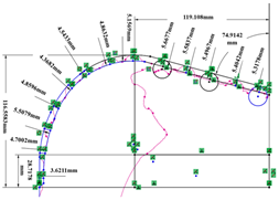
Applsci 14 04370 i005
Diameter preservingThe design parameters for diameter preservation analyzed in the analysis of rock-breaking structure characteristics of drill bits include diameter preservation length and diameter preservation width; The measurement of diameter preservation length requires the use of sketches, the identification of diameter preservation and gauge characteristics using experience, and the measurement of diameter preservation data.Applsci 14 04370 i006
The measuring of the diameter preserving width is to use the surface sketch to intercept the point cloud of the cross section of the diameter, and to measure the fitting.Applsci 14 04370 i007
The spiral Angle of the gauge is produced by smearing the “domain”, and the gauge side is automatically fitted, and the outline of a single gauge is captured by the surface sketch and measured.Applsci 14 04370 i008
BladeThe thickness of the blade is obtained by using a surface sketch to capture the cross-sectional contour data points at the blade, fitting the edges on both sides of the blade, and measuring the length of its connecting line, which is the blade thickness.Applsci 14 04370 i009
Cutter structure parametersThe structural parameters of the analyzed cutters include the diameter, the cutting angle range, the cutter edge height, and the cutter shape. The height of the cutter edge is measured based on the drawn drill bit profile curve and blade curve, and the judgment of the cutter shape can be directly obtained through observation. The cutter diameter was measured using a “ domain “ smear fitted cylinder.Applsci 14 04370 i010
Before measuring the cutting angle of cutters, it is necessary to construct a blade surface, which is used as the reference for measuring the cutting angle of cutters. For conventional cylindrical cutters, the cutting angle of the cutter is determined by measuring the angle between the fitted cutter surface and the corresponding blade flank surface by applying a “domain” fitting to the surface of the cutter. For special-shaped cutters, the cylindrical surface of the cutter is fitted by applying “domain” to obtain the axis of the cylindrical surface. The angle between the axis and the corresponding blade surface is measured as the residual angle of the cutting angle of the cutter.Applsci 14 04370 i011

Appendix B

Algorithm A1. The calculation code of Spearman rank correlation coefficient.
%% Clear all variables in the workspace.
clear all;
clc;
%% Load variables.
load Inputdata.mat; % Load drill bit structure output variables.
load Outputdata.mat; % Load drill bit footage and ROP output variables.
%% Calculate the Spearman correlation coefficients.
for i = 1: size (Outputdate,2); % The “size” represents the number of columns in a two-dimensional matrix of input variables.
   for j = 1: size (Inputdata,2); % The “size” represents the number of columns in a two-dimensional matrix of output variables.
   Data= [Inputdata (:, j) Outputdate (:, i)]; % Create a 2-column matrix DATA, with the first column being the j-th column of the input variable and the second column being the i-th column of the output variable.
   Spearman = corr (Data, ‘type’, ‘Spearman’); % Calculate the correlation coefficient of Spearman type based on the established matrix.
   S (j,i) = Spearman(1,2); % Establish a matrix S with 1 row and 2 columns, corresponding to two Spearman correlation coefficients for each drill bit structure with respect to footage and drilling speed.
  end
end

Appendix C

Algorithm A2. The prediction program code based on the BP neural network algorithm.
%% Clear all variables in the workspace.
clear all;
clc;
%% Training/testing set generation.
load Inputdata.mat;
load Outputdata.mat;
pca_gj = data (:,:);
temp = randperm (size (pca_gj, 1)); % Randomly generate training and testing sets.
% Create training set.
P_train = pca_gj (temp (1: 4), :)’;
T_train = output (temp (1: 4), :)’;
% Create test set.
P_test = pca_gj (temp (5: end), :)’;
T_test = output (temp (5: end), :)’;
N = size(P_test,2);
%% BP neural network creation, training, and simulation testing.
% Create a network.
net = newff (P_train, T_train, 9);
% Set training parameters.
net.trainParam.epochs = 10,000; % Training frequency, set to 10,000 times here.
net.trainParam.goal = 1 × 10⁻³; % The minimum error of the training objective is set to 1 × 10⁻³ here.
net.trainParam.lr = 0.01; % Learning rate, set to 0.01 here.
% Training Network
net = train (net, P_train, T_train);
% Simulation test
T_sim_bp = sim(net,P_test);
%% performance evaluation
% relative error
error_bp(1,:) = abs(T_sim_bp(1,:)—T_test(1,:))./T_test(1,:);
error_bp(2,:) = abs(T_sim_bp(2,:)—T_test(2,:))./T_test(2,:);
% coefficient of determination R^2
R2_bp(1) = (N * sum(T_sim_bp(1,:) .* T_test(1,:))—sum(T_sim_bp(1,:)) * sum(T_test(1,:)))^2/((N * sum((T_sim_bp(1,:)).^2)—(sum(T_sim_bp(1,:)))^2) * (N * sum((T_test(1,:)).^2)—(sum(T_test(1,:)))^2));
R2_bp(2) = (N * sum(T_sim_bp(2,:) .* T_test(2,:))—sum(T_sim_bp(2,:)) * sum(T_test(2,:)))^2/((N * sum((T_sim_bp(2,:)).^2)—(sum(T_sim_bp(2,:)))^2) * (N * sum((T_test(2,:)).^2)—(sum(T_test(2,:)))^2));
% Result comparison
result_bp = [T_test’ T_sim_bp’ error_bp’]
%% Draw a picture
Figure (1)
Plot (1: N, T_test (1, :), ‘b: *’, 1: N, T_sim_bp (1, :), ‘r-o’)
Legend (‘ true value ‘, ‘BP predicted value ‘)
xlabel (‘forecasting sample ‘)
ylabel (‘ Predicted value 1’)
Figure (2)
Plot (1: N, T_test (2, :), ‘b: *’, 1: N, T_sim_bp (2, :), ‘r-o’)
Legend (‘ true value ‘, ‘BP predicted value ‘)
xlabel (‘forecasting sample ‘)
ylabel (‘ Predicted value 2’)

References

  1. Guo, T. Key geological issues and main controls on accumulation and enrichment of Chinese shale gas. Pet. Explor. Dev. 2016, 43, 349–359. [Google Scholar] [CrossRef]
  2. Xu, Q.; Xu, F.; Jiang, B.; Zhao, Y.; Zhao, X.; Ding, R.; Wang, J. Geology and transitional shale gas resource potentials in the Ningwu Basin, China. Energy Explor. Exploit. 2018, 36, 1482–1497. [Google Scholar] [CrossRef]
  3. Li, S.Z.; Zhou, Z.; Nie, H.K.; Zhang, L.F.; Song, T.; Liu, W.B.; Li, H.H.; Xu, Q.C.; Wei, S.Y.; Tao, S. Distribution characteristics, exploration and development, geological theories research progress and exploration directions of shale gas in China. China Geol. 2022, 5, 110–135. [Google Scholar] [CrossRef]
  4. Yu, G.; Liu, H.; Li, H.; Fang, Y.; Luo, L. Prediction on peak production of shale gas, southern Sichuan Basin. Nat. Gas Explor. Dev. 2023, 46, 97. [Google Scholar]
  5. Melikoglu, M. Geothermal energy in Turkey and around the World: A review of the literature and an analysis based on Turkey’s Vision 2023 energy targets. Renew. Sustain. Energy Rev. 2017, 76, 485–492. [Google Scholar] [CrossRef]
  6. Hu, X.; Xie, J.; Cai, W.C.; Wang, R.; Davarpanah, A. Thermodynamic effects of cycling carbon dioxide injectivity in shale reservoirs. J. Pet. Sci. Eng. 2020, 195, 107717. [Google Scholar] [CrossRef]
  7. Lei, Q.; Xu, Y.; Yang, Z.; Cai, B.; Wang, X.; Zhou, L.; Liu, H.; Xu, M.; Wang, L.; Li, S. Progress and development directions of stimulation techniques for ultra-deep oil and gas reservoirs. Pet. Explor. Dev. 2021, 48, 221–231. [Google Scholar] [CrossRef]
  8. Ma, X.H.; Wang, H.Y.; Zhou, S.W.; Shi, Z.S.; Zhang, L.F. Deep shale gas in China: Geological characteristics and development strategies. Energy Rep. 2021, 7, 1903–1914. [Google Scholar] [CrossRef]
  9. Cheng, Z.; Li, G.S.; Huang, Z.W.; Sheng, M.; Wu, X.G.; Yang, J.W. Analytical modelling of rock cutting force and failure surface in linear cutting test by single PDC cutter. J. Pet. Sci. Eng. 2019, 177, 306–316. [Google Scholar] [CrossRef]
  10. Song, X.; Pei, Z.; Wang, P.; Zhang, G. Intelligent prediction for rate of penetration based on support vector machine regression. Xinjiang Oil Gas 2022, 18, 14–20. [Google Scholar]
  11. Yan, J. Study on Optimization of PDC Bit Based on BP Neural Network. Master’s Thesis, China University of Petroleum (East China), Dongying, China, 2019. [Google Scholar]
  12. Shi, X.; Liu, G.; Gong, X.L.; Zhang, J.L.; Wang, J.; Zhang, H.N. An Efficient Approach for Real-Time Prediction of Rate of Penetration in Offshore Drilling. Math. Probl. Eng. 2016, 2016, 3575380. [Google Scholar] [CrossRef]
  13. Bourgoyne, A.T.; Young, F.S. A Multiple Regression Approach to Optimal Drilling and Abnormal Pressure Detection. Soc. Pet. Eng. J. 1974, 14, 371–384. [Google Scholar] [CrossRef]
  14. Wang, K.; Wei, F. Applications of Logging Information in Predicting Formation Anti-Drilling Parameters. Pet. Drill. Tech. 2003, 31, 61–62. [Google Scholar]
  15. Li, C. Study of method for predict rate of penetration based of multiple regression analysis. Sci. Technol. Eng. 2013, 13, 1740–1744. [Google Scholar]
  16. Mazen, A.Z.; Rahmanian, N.; Mujtaba, I.; Hassanpour, A. Prediction of Penetration Rate for PDC Bits Using Indices of Rock Drillability, Cuttings Removal, and Bit Wear. SPE Drill. Complet. 2020, 36, 320–337. [Google Scholar] [CrossRef]
  17. Chen, H.D.; Jin, Y.; Zhang, W.D.; Zhang, J.F.; Ma, L.; Lu, Y.H. Deep Neural Network Prediction of Mechanical Drilling Speed. Energies 2022, 15, 3037. [Google Scholar] [CrossRef]
  18. Aalizad, S.A.; Rashidinejad, F. Prediction of penetration rate of rotary-percussive drilling using artificial neural networks—A case study. Arch. Min. Sci. 2012, 57, 715–728. [Google Scholar]
  19. Su, X.; Sun, J.; Gao, X.; Wang, M. Prediction method of drilling rate of penetration based on GBDT algorithm. Comput. Appl. Softw. 2019, 36, 87–92. [Google Scholar]
  20. Ahmed, O.S.; Aman, B.M.; Zahrani, M.A. Stuck Pipe Early Warning System Utilizing Moving Window Machine Learning Approach. In Proceedings of the Abu Dhabi International Petroleum Exhibition & Conference, Abu Dhabi, United Arab Emirates, 11–14 November 2019. [Google Scholar]
  21. Liu, S.; Sun, J.; Gao, X.; Wang, M. Analysis and Establishment of Drilling Speed Prediction Model for Drilling Machinery Based on Artificial Neural Networks. Comput. Sci. 2019, 46, 605–608. [Google Scholar]
  22. Diaz, M.B.; Kim, K.Y.; Shin, H.-S.; Zhuang, L. Predicting rate of penetration during drilling of deep geothermal well in Korea using artificial neural networks and real-time data collection. J. Nat. Gas Sci. Eng. 2019, 67, 225–232. [Google Scholar] [CrossRef]
  23. Hazbeh, O.; Aghdam, S.K.; Ghorbani, H.; Mohamadian, N.; Alvar, M.A.; Moghadasi, J. Comparison of accuracy and computational performance between the machine learning algorithms for rate of penetration in directional drilling well. Pet. Res. 2021, 6, 271–282. [Google Scholar] [CrossRef]
  24. Lawal, A.I.; Kwon, S.; Onifade, M. Prediction of rock penetration rate using a novel antlion optimized ANN and statistical modelling. J. Afr. Earth Sci. 2021, 182, 104287. [Google Scholar] [CrossRef]
  25. Zhang, H.; Zhang, G.; Wang, G.; Wang, L.; Liu, Y.; Ren, Y.; Zheng, S. Classification and Prediction Method for ROP Based on Genetic Algorithm Optimization Random Forest Model. Sci. Technol. Eng. 2022, 22, 15572–15578. [Google Scholar]
  26. Alkinani, H.H.; Al-Hameedi, A.T.T.; Dunn-Norman, S. Data-driven recurrent neural network model to predict the rate of penetration. Upstream Oil Gas Technol. 2021, 7, 100047. [Google Scholar] [CrossRef]
  27. Burghes, D.N. Teaching Spearman’s Rank Correlation Coefficient. Teach. Stat. 2007, 15, 68–69. [Google Scholar] [CrossRef]
  28. Hauke, J.; Kossowski, T. Comparison of Values of Pearson’s and Spearman’s Correlation Coefficients on the Same Sets of Data. Quageo 2011, 30, 87–93. [Google Scholar] [CrossRef]
Figure 1. Rank correlation coefficient of structural characteristics from Shaximiao Formation to Ziliujing Formation in the second spud of Luzhou Block.
Applsci 14 04370 g001
Figure 2. Rank correlation coefficient of structural characteristics from Xujiahe Formation in the third spud of Luzhou Block.
Applsci 14 04370 g002
Figure 3. Rank correlation coefficient of structural characteristics from Qixia Formation to Shiniulan Formation in the fourth spud of Luzhou Block.
Applsci 14 04370 g003
Figure 4. Schematic diagram of BP neural network for prediction of ROP and footage.
Applsci 14 04370 g004
Figure 5. Determination coefficient of prediction model under different number of neurons in hidden layer.
Applsci 14 04370 g005
Figure 6. Prediction results of BP neural network: (a) Shaximiao Formation to Ziliujing Formation and (b) Xujiahe Formation.
Applsci 14 04370 g006aApplsci 14 04370 g006b
Table 1. Analysis results of PDC bit structure characteristics.
Footage
(m)
ROP
(m/h)
Size
(mm)
Model
Name
Crown Top Rotation Radius
(mm)
Gauge Diameter Length
(mm)
Blade NumberCrown Top Blade Thickness
(mm)
Gauge Length
(mm)
Gauge Width
(mm)
Nozzle NumberEquivalent Diameter of Nozzle
(mm)
Radial Flow Channel Depth
(mm)
76218.59406.4SD6647VZ155.0724.48665.2246.5658.48935.2169.42
7727.21406.4SD6648BZ166.7431.77669.458.766.881244102.87
483.579.94406.4TS1665B167.2327.64670.58561.346.5931.8351.63
10659.22406.4TS616163.1424.32661.91573.1745.71931.8356.27
82111.25406.4TS1656B161.4728.59576.10573.958.44931.8351.75
513.512.8406.4T166517428.44670.51570.6550.78931.8340.42
347.3313.99406.4TS1666B159.436.34667.30575.4748.89931.8361.89
42211.68406.4TS1655B17553.6574.41574.557.3840.4150.7
305.649.952406.4T1655BS160.261.7583.02104.175.6840.4165
67713.24406.4CAS6164N146.163.04669.9312793.84935.7281.79
541.639.15406.4CAS6164W151.9562.97672.9412798.41935.7284.02
385.9714.48406.4DS653AB152.263.41568.895120.364.32840.4172.86
6018.84406.4HS5163BU167.9851.21565.27561.9160.331040.1698.28
442.7511.81406.4HS5163BMK160.6755.91570.50565.3770.68840.4176.6
46110.72406.4HS6163BU177.1238.6653.54556.9274.56940.1693.39
563.7111.8406.4KS1662DGRS12629.75665.215108.476.93931.8356.07
420.611.32406.4ES1626ET158.563671.68134.476.53933.3879.2
6446.92311.2SD6542B111.1825.21558.58554.6962.54844.959.31
3887.76311.2SD6632BZ88.2937.18652.3389.1372.955944.5659.16
4156.39311.2SD6642B115.9132.2660.59574.3252.18950.8559.64
6255.515311.2TS1655BP12054.4559.578.651.4840.4158.6
543.15.71311.2TS1655B130.536552.3555.343.574248.8
387.64.87311.2T1665135.446.865563.444933.3845.3
327.16.23311.2TS616123.9346.19653.68568.3846.19933.3846.75
1373.61311.2TS1653107.8450.24556.564.150.26840.4153.74
188.676.7311.2TS1653B110.9544.09558.6968.5944.2840.4156.63
192.634.8311.2TS1655BTS106.751.972561.78577.1951.97746.248.74
5899.28311.2DS653H118.3357.39558.6868.9657.23833.6860.84
2236.43311.2DS664H111.7536.15655.6975.0937.86933.3863.84
2244.96311.2DS674H108.0152.08740.9961.5351.951040.1662.14
2174.43311.2DM653H76.8439.82563.81569.7940.5874278.76
338.756.21311.2KMD1662ART124.657.6662.685109.9104938.157.08
385.266.87311.2KS1652DFGRT121.552560.4158276.9938.166.2
120.55.13311.2KS1652FGRY125105654.395126108840.4154.72
411.756311.2ES1656TEU125.473.166598.755.64938.166
5697.16311.2ES1635E11249.07558.4597.878.12844.964.4
10218.59215.9ES1655L87.751.4547.876.6661.05746.235.6
Table 2. The specific stratification results for Luzhou Block in Sichuan Province.
The StageThe Rock StrataThe Well Depth
Second spud-1Shaximiao Formation~Ziliujing Formation
(Lianggaoshan Formation)
80 m~900 ± 50 m
Second spud-2Ziliujing Formation~Xujiahe Formation900 ± 50 m~1100 ± 50 m
Third spud-1Xujiahe Formation1100 ± 50 m~1600 ± 50 m
Third spud-2Jialingjiang Formation~Longtan Formation
(Feixianguan Formation, Changxing Formation)
1600 ± 50 m~2600 ± 50 m
Third spud-3Maokou Formation~Qixia Formation2600 ± 50 m~2950 ± 50 m
Fourth spud-1Qixia Formation to Shiniulan Formation
(Liangshan Formation~Hanjiadian Formation)
2950 ± 50 m~3500 ± 50 m
Fourth spud-2Shiniulan Formation~Longmaxi Formation3500 ± 50 m~5900 ± 50 m
Table 3. The MSE results for calculating the prediction model of ROP (m/h).
Shaximiao Formation to Ziliujing FormationXujiahe Formation
Number of Hidden Layer NeuronsMean Squared Error (MSE)Number of Hidden Layer NeuronsMean Squared Error (MSE)
53.53751.545
63.82461.279
72.41271.185
82.28580.962
91.85690.804
101.562100.787
111.884110.583
122.050120.671
131.968130.727
Disclaimer/Publisher’s Note: The statements, opinions and data contained in all publications are solely those of the individual author(s) and contributor(s) and not of MDPI and/or the editor(s). MDPI and/or the editor(s) disclaim responsibility for any injury to people or property resulting from any ideas, methods, instructions or products referred to in the content.

