1. Introduction
As the integration of sensing and communication technologies rapidly advances, the terahertz (THz) frequency band (0.1–10 THz) has emerged as a pivotal frontier for both domains, presents opportunities in achieving high-data-rate communication and precise environmental sensing [
1,
2]. These features promise a significant advancement in capabilities for 6G integrated sensing and communication (ISAC) technology [
3], autonomous vehicles [
4], and vehicular communication networks (VCN) [
5]. In such integrated systems, the role of environmental sensing becomes important increasingly. They require swift and precise perception of the environment to adapt in real-time environmental variations and enhance communication and/or control system stability [
6,
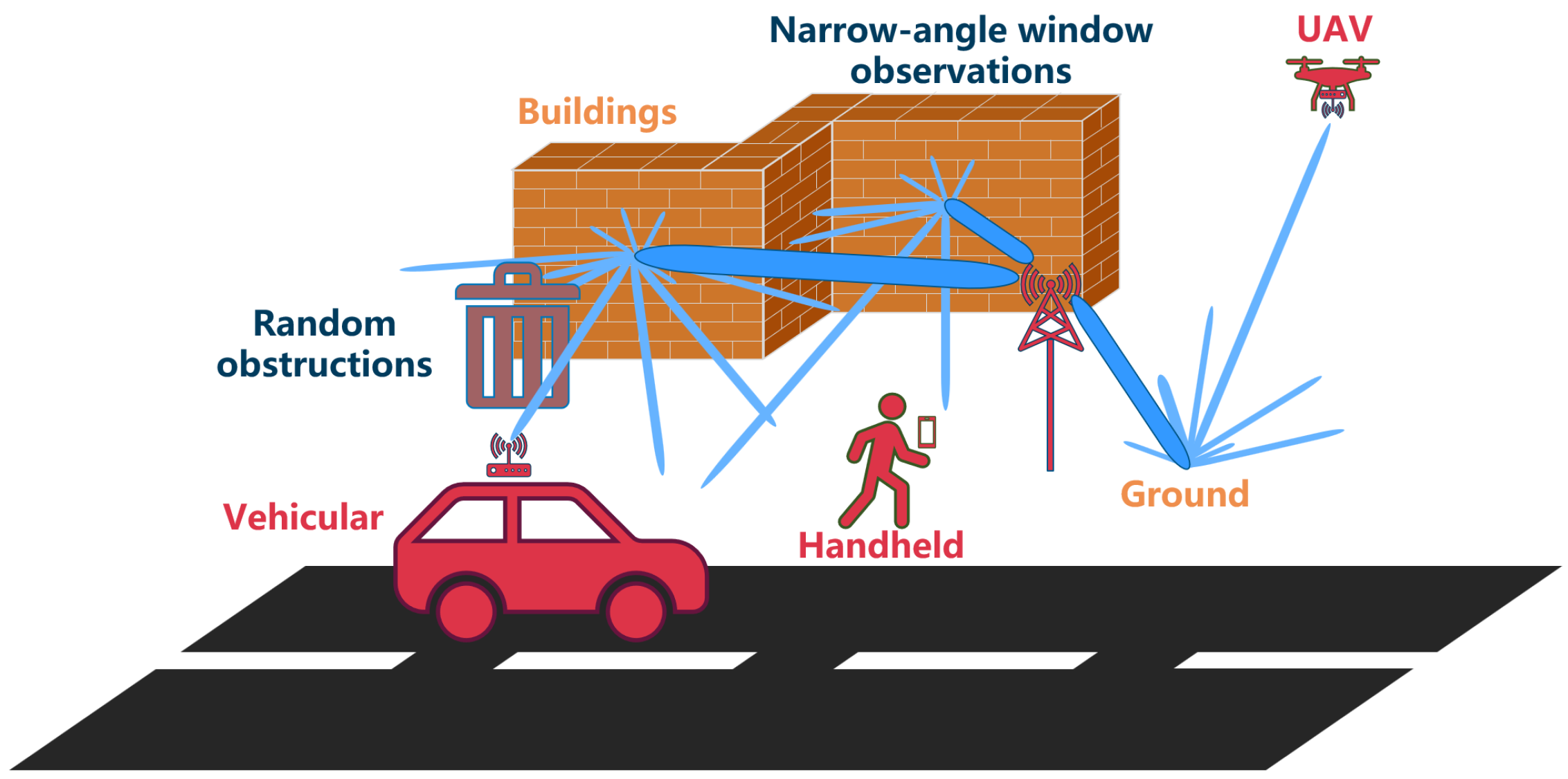
7]. In these scenarios, accurate recognition of surface roughness emerges as a critical environmental parameter, as shown in
Figure 1. The scattering characteristics of wireless channels, for example, are profoundly influenced by the texture of surrounding surfaces [
8], and then the control system of autonomous vehicles must adapt to the roughness of the terrain [
9]. Terahertz frequencies are inherently sensitive to surface granularity, offering a potent advantage in addressing these challenges [
10]. In other words, they can decode intricate details of surrounding surfaces, yielding distinct signatures within their scattering spectra [
11,
12]. This makes them invaluable for non-invasive surface texture assessments.
There have been diverse strategies, such as Kirchhoff theory [
13], Rayleigh roughness theory [
14], the time-of-flight method [
15], etc., developed for surface texture modeling and recognition, relying on numerical scattering models [
16,
17]. These methods require complicated modeling trajectories and are anchored in approximate and idealized postulates, which often fail to accurately capture real-world complexities. Other techniques harness the richness of THz imaging features, predominantly integrating deep learning frameworks [
9,
18,
19]. While all these approaches are adept in low-speed scenarios, they are not well suited for high-speed conditions, where numerical computations become impractical and radar imagery becomes prohibitively resource intensive.
In high-speed scenarios, static equipment positioning is unfeasible, and sampling must transpire dynamically. This introduces tailing effect, which means the data captured at a specific time and angle include traces from previous conditions. The magnitude of the tailing effect increases with speed, leading to directional spectral biases and attenuation of spectral details. In addition, high-speed sampling introduces additional challenges, such as random occlusions, high-speed sparse data, and narrow-angle window observations, which render conventional methodologies inadequate [
20]. To overcome these challenges, we propose a deep learning-driven paradigm for surface texture recognition in high-speed scenarios in this work, which has already been demonstrated as its prowess in pragmatic terahertz applications such as imaging [
21], synthetic aperture radar (SAR) [
22], and hyperspectral modalities [
23]. This paradigm necessitates an authentic, diverse, and concise dataset for model training, ensuring its alignment with real-world scenarios, robust generalization capabilities, and stability in complex environments. Thus, we designed a data recording platform that emulates real-world dynamics. We also fabricated several kinds of rough surface samples, characterized them by high-fidelity 3D scanning, and acquired a large amount of high-speed scattering data. To strengthen data heterogeneity, we focused on localized sample regions and further enriched them with diverse data processing and augmentation strategies to sculpt the dataset.
The remainder of this article is laid out as follows:
Section 2 gives a thorough description on the data collection platform, which includes how we set up our experiments and the system we used to control them.
Section 3 provides a detailed depiction of how we created and assessed the rough surfaces that we used as samples.
Section 4 explains how we recorded the data needed to train our algorithms.
Section 5 describes how we designed the algorithm that our network employed.
Section 6 discusses the experiments we conducted using deep learning and delves into what the results mean. Finally,
Section 7 concludes the entire work. We think that this work presents a significant advancement in the field of surface texture recognition with terahertz frequencies, enabling robust and reliable operation in high-speed scenarios. We also think that it opens up new possibilities for a wide range of applications, including autonomous driving, environmental monitoring, and industrial inspection.
2. Data Sampling Platforms
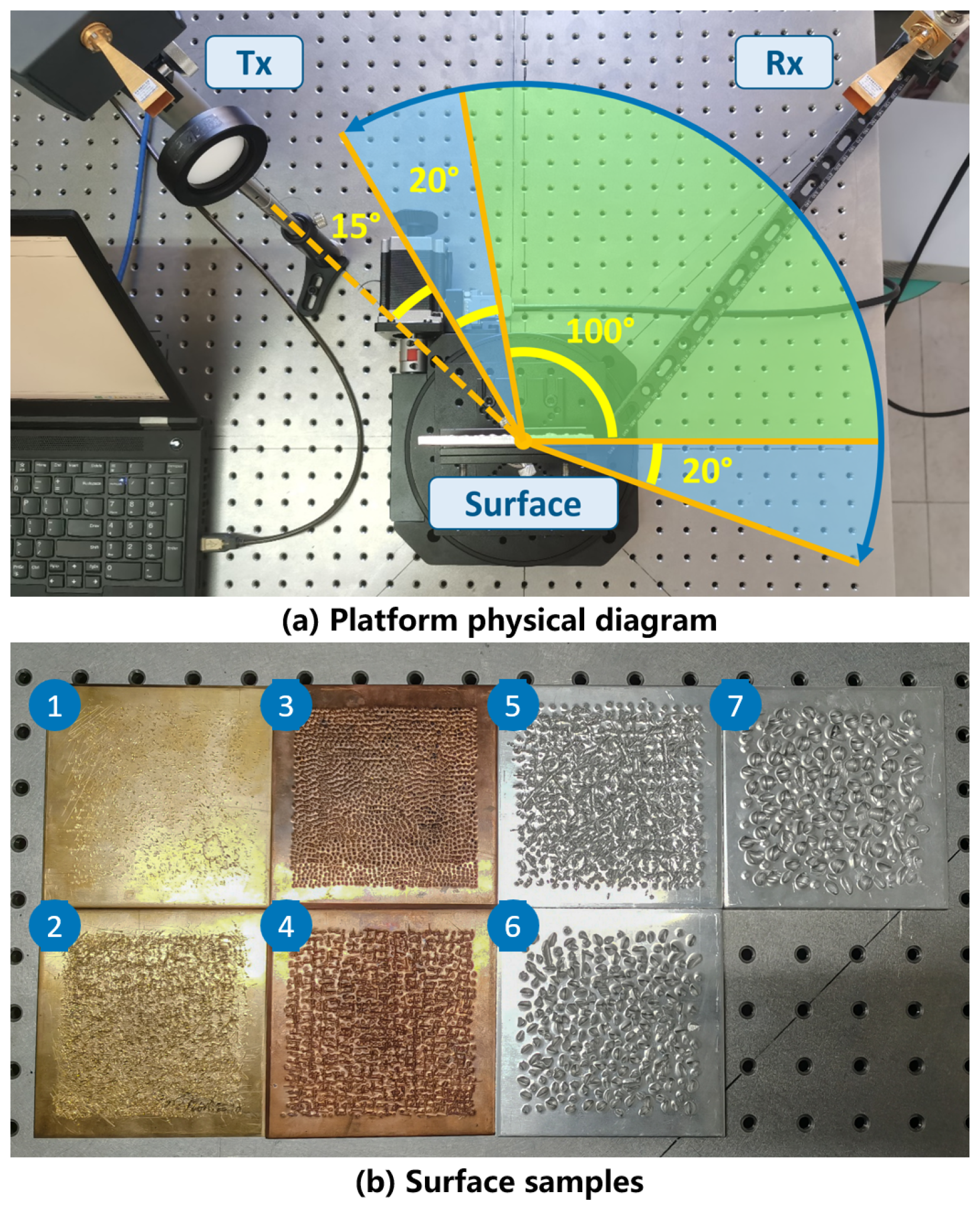
To meet the demands of real-world applications, we fabricated a high-speed sampling platform, depicted in
Figure 2a. This platform is designed to fulfill the dual criteria of rapid rotation and high precision, achieved through a fully automated programming-driven sampling system. Its core is a high-precision electrical control rotational stage powered by a 57-step stepper motor and governed by a worm gear structure. The motor, with a step angle of 1.8° and a mechanical transmission ratio of 1:180, confirms the rotational stage with a minimum rotation angle of 0.01°. This makes its precision and alignment under the measurement requirements.
The experimental setup involved affixing the receiver (Rx) onto the rotational stage via an extended rail, placing the rough surface sample at the rotational stage’s epicenter, and situating the transmitter (Tx) at a 45 incident angle. We designed such a setup to emulate scenarios of collaborative perception to avoid the self-interference faced in independent perception [
24,
25] such as a base station emitting perception signals that are reflected by sensed targets and received by terminals. The spatial arrangement had the transmitter and receiver positioned 36 cm and 38 cm away from the sample’s geometric center, respectively. The transmission assembly comprised a signal generator (Ceyear 1465D), a frequency multiplier module (Ceyear 82406B), and a horn antenna. The signal generator (Ceyear 1465) has the capability to generate signals up to 20 GHz, which were then up-converted to the 110–170 GHz range using the Ceyear 82406D. The receiver employs an identical horn antenna to capture signals and forwards them to a power sensor (Ceyear 71718) for signal detection with a single sampling time of 50 ms. This setup allows us to analyze the variations in signal strength and pattern as influenced by different levels of surface roughness [
26], enabling the correlation between the received power data and the physical texture characteristics of the surfaces. To enhance focusing, a lens with a 10cm focal length was strategically positioned in front of Tx, aligning with the focal point. Throughout the sampling process, while Tx and the surface sample remained stationary, Rx embarked on a circular trajectory around the sample, instigating variations in reflection angles. Both Tx and Rx are fixed within a horizontal plane, which is not fully representative of practical situations where an elevation angle may be often present [
26,
27]. However, for environmental sensing in the real world, we think that a near-zero elevation angle can be sufficient in most cases.
The electrical control rotational stage was exercised through a serial port protocol, ensuring continuous motion data monitoring. Concurrently, LAN and SCPI protocols were deployed as interface protocols connecting the terahertz signal generator and power meter. Through the utilization of these protocols to transmit our predefined commands, control over both devices is facilitated. The amalgamation of these components was seamlessly orchestrated using Python 3.9, which facilitated interface calls, ensured time synchronization, governed sampling control, and oversaw data storage operations. This sophisticated platform guarantees an automatic and highly efficient data acquisition process with a communication latency less than 10 ms.
3. Surface Sample Preparation
Data are paramount in the realm of neural networks. Aiming for effective performance on real-world surfaces with unknown roughness, it is important to improve the generalization capabilities of limited set of surface samples with different levels of roughness. This requires our samples to embody typical characteristic properties. Due to the difficulties in obtaining enough data for our investigation, we chose metal surfaces for our primary samples, due to their excellent reflective properties and a diverse range of hardness. We applied different processes to forge surfaces with different levels of roughness, as shown in
Figure 2b.
To create smoother surfaces resembling scratches and minor textural variations on office desks or brushed finishes, we used small-diameter rectangular and cylindrical chisels on harder brass materials to create two distinct surfaces. Surface-1 features scratches and minor abrasions, while Surface-2 predominantly features scratches with shallow grooves. To create rougher surfaces with inherent natural textures, such as wood grain and genuine leather patterns, we used conical and medium-diameter rectangular chisels on materials of moderate hardness, specifically copper. Surface-3 is composed of dense conical pits, emulating certain grid-like textures. Surface-4, derived from Surface-3, incorporates deeper grooves to mimic deep leather textures. Given that rougher surfaces often exhibit more pronounced relief structures, we used larger-diameter conical and rectangular chisels on softer aluminum sheets to produce three additional surfaces. Surface-5 is an enhanced version of Surface-4. Surfaces-6 and -7, in contrast to the previous methods of vertical carving, employ lateral force application to create substantial depressions and peaks in the structure. All these surface samples possess a large size, measuring 100 mm × 100 mm. Within this area, the central region of 80 mm × 80 mm exhibited the roughness characteristics. We used a grid counting method to ensure maximum uniformity in the local roughness within this region. Such a large surface area endows the dataset with a richer diversity of data featuring similar numerical roughness but varied structures.
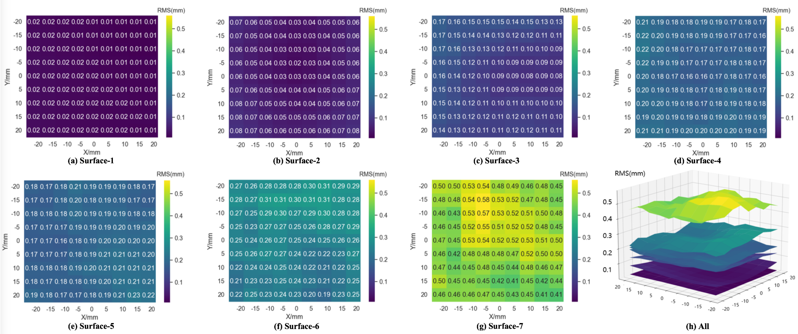
For accurate characterization of the surface samples, we conducted a comprehensive three-dimensional (3D) laser scanning (SCANTECH IREAL2E) using high-precision techniques to reconstruct all the surfaces. We utilized an industrial-grade handheld 3D laser scanner with a scanning precision of 0.02 mm and a volumetric accuracy of 0.03 mm/m. Each metal surface underwent scanning to produce cloud with at least two million points, effectively representing the roughness of various local areas on the surface. We used the standard deviation of the surface height variation (RMS) as a quantitative measure of surface roughness [
28]. The ensuing results, detailed in
Figure A1 of the
Appendix A, reveal that our samples of rough surfaces manifest several characteristic traits: (1) Minimal overlap of roughness between different surfaces, which is essential for subsequent classification tasks, yielding classification results that can be uniquely mapped back to a specific range of roughness. (2) Variability in roughness across different areas within a single surface. This enriches the dataset and enhances the model’s ability to generalize. (3) Existence of regions with comparable levels of roughness yet differing in shapes and quantities. This further contributes to the overall data richness.
4. Dataset Acquisition and Composition
The data acquisition was conducted by employing the platform and surfaces as in
Figure 2. In low-speed scenarios, scatter sampling is typically performed at one angle per pause (of the rotational stage), ensuring precision and stability. However, high-speed scenarios require continuous sampling, which introduces a trailing effect, as we mentioned in
Section 1. To emulate real-world high-speed conditions, we continuously sampled while the Rx rotated without pausing. We set the sampling speed to match the rotational stage’s safety speed limit while maintaining a minimum angular distance of 15° between the Rx and Tx. We also included acceleration and deceleration zones (20°) at the beginning and end of the motion. The sampling strategy was meticulously designed to ensure comprehensive data coverage across all surface types. Each rotation cycle was programmed to capture data systematically around the entire circumference of the sample, ensuring no angular sector was underrepresented. This systematic collection was essential to construct a dataset that accurately represents the variability inherent in real-world surface textures.
In order to improve the robustness and generalization ability of our model, we need a diverse dataset from a limited number of rough surface samples. We achieved this by methodically moving an incident beam across the surface to gather sufficient data for model training. Considering the illumination area (by the channel beam) with a diameter of 3 cm on the surface, we moved the beam in both horizontal and vertical dimensions in 5 mm increments. With each movement, we collected a set of scattering data, referred to as a sampling sequence. Additionally, to mitigate the peak displacement resulting from the tailing effect, we rotated our receiver (RX) in both clockwise and counterclockwise directions at each sampling location. By doing so, we acquired 72 sampling sequences for each surface. In total, this process yielded 504 unique sampling sequences across seven different surfaces.
To demonstrate the effect of the rotation speed of the stage and sampling parameters (average number and query interval), we conducted a comprehensive analysis using a range of speed and parameter settings, as summarized in
Table 1. Rotation speed refers to the speed at which the motorized rotation stage moves during the uniform motion phase. The average number represents the numerical configurations for the built-in averaging feature of the sampling apparatus. It has been confirmed that its variation within a numerical range has a negligible impact on the final classification F1 score. Query frequency indicates how often the Python main control program retrieves data from the sampling device. It can be seen that rotation speed and query interval (frequency) can affect the cumulative length of the acquired sequences, including data from the acceleration and uniform motion zones near the Tx side.
5. Scenario and Network Analysis
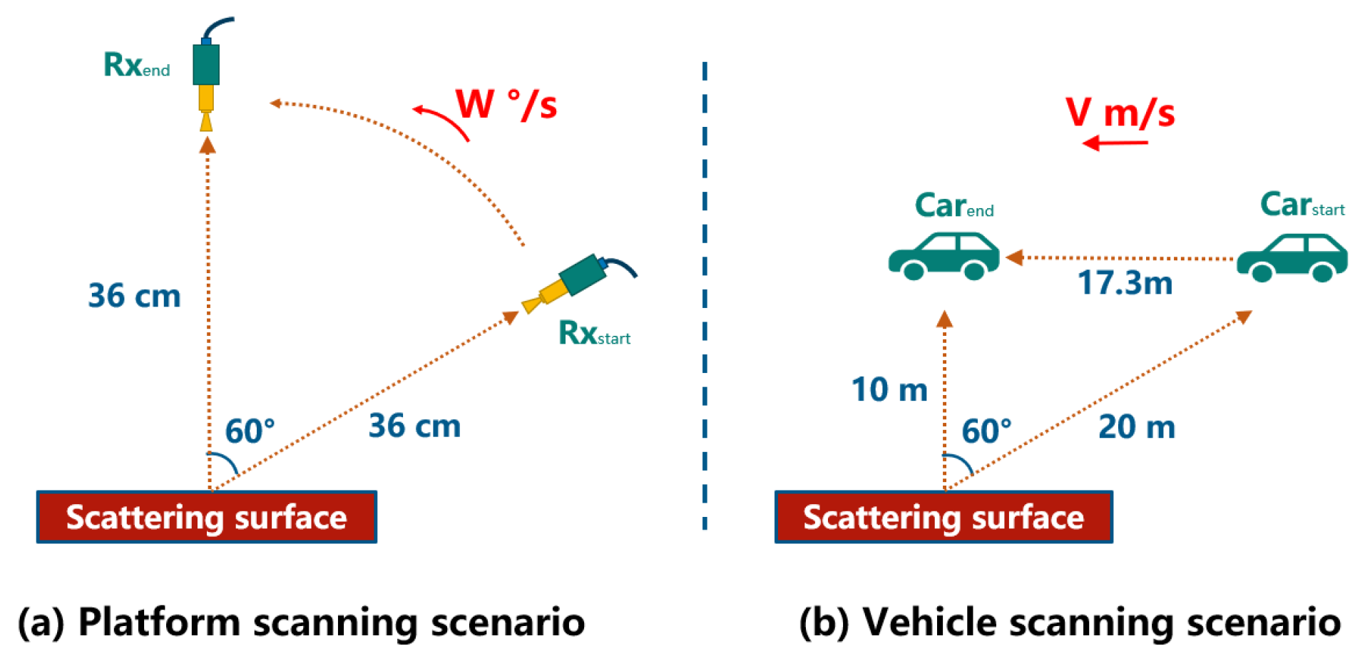
We described the actual collaborative perception scenario that our experimental setup aims to emulate, as shown in
Figure 3. The target surface reflects signals launched by a base station to a terminal (terahertz sensor) on a moving vehicle. The vertical distance between the surface and the vehicle’s trajectory is assumed to be 10 m. To avoid the challenges of excessive distances, we focused on a detection range where the incident angle does not exceed
. This corresponds to a horizontal span of 17.3 m. With a turntable rotating at an angular speed of
/s, it takes 6 s to traverse a range of
. This corresponds to a vehicular speed of approximately 10 km/h, which is similar to the pace of a pedestrian. For a rotational speed of
/s, the emulated vehicular speed increases to around 20 km/h, which is similar to the speed of a vehicle in low-speed cruising.
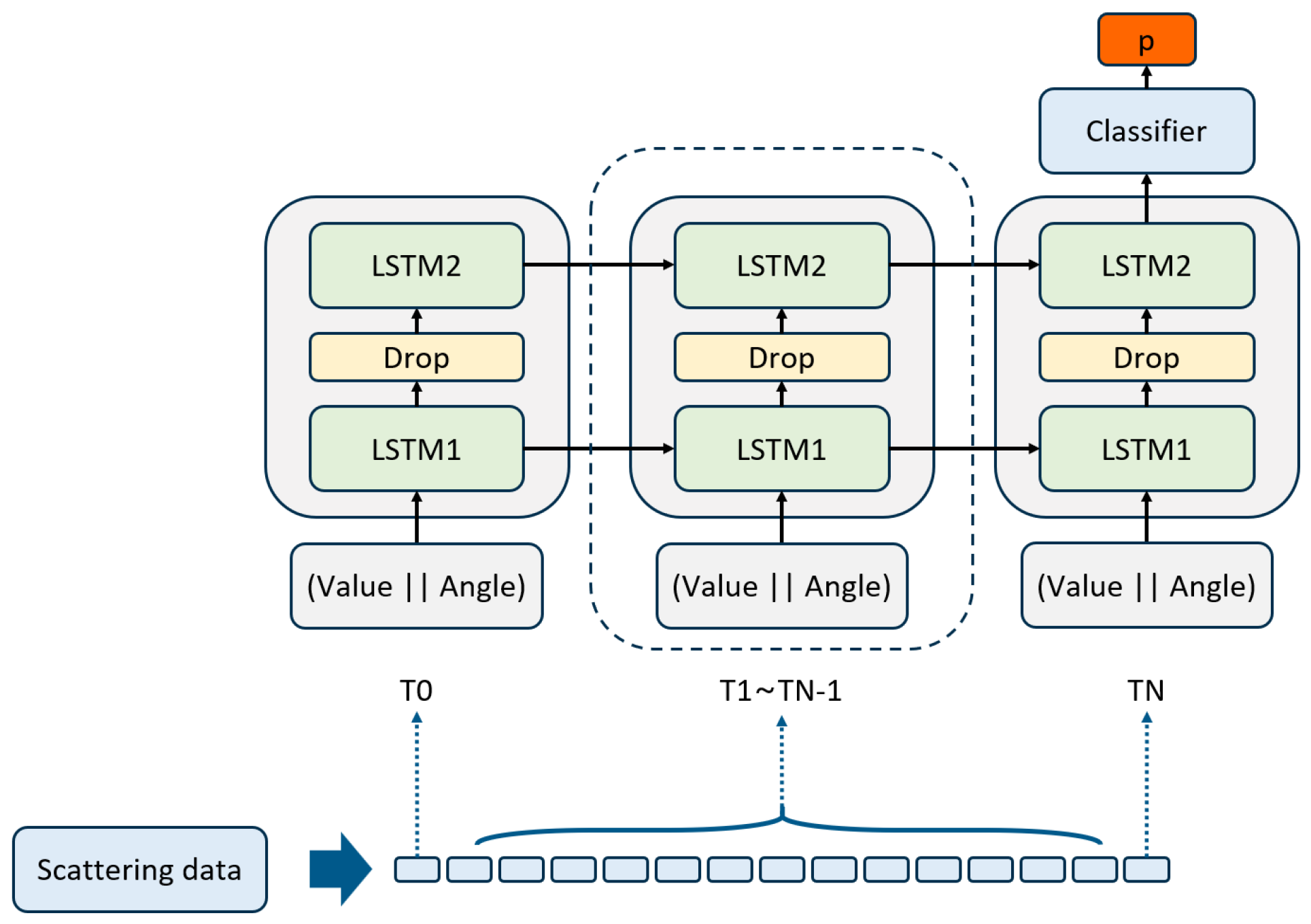
Using the raw dataset we collected, we have performed a classification task to distinguish between different rough surfaces. The model takes scattering sequence data (X) from a specific position on a surface as input. Each sequence comprises scattering data captured at different angles, represented as , where N is the number of sampling points in one sequence. Due to the complexities of real-world high-speed scenarios, it is impractical to assume that the data points adhere to a specific angle-related sequence. Therefore, it is necessary to combine the numerical representations of the sampling points and scattering angles, resulting in the representation . The model’s output is a probability distribution over different surface categories, expressed as , where M is the total number of surface categories.
To enhance the execution of sequence tasks, addressing the inherent variability in sequence lengths is crucial; we use a highly stable LSTM model [
29], which is a type of recurrent neural network (RNN). LSTM models have unique gated structures that effectively filter and process information, mitigating redundancy in memory storage. This architecture is particularly well-suited for tasks involving lengthy sequences and it also solves the vanishing gradient problem that is prevalent in traditional RNNs. The LSTM architecture has a memory cell (
) as well as three key gate mechanisms: the input gate (
), the output gate (
), and the forget gate (
). At each time step, the model updates the states of these gates based on the current input and output from the previous time step. This process determines which pieces of information should be retained, discarded, or produced as output. The variable
represents the input information.
with
(.) representing a logistic sigmoid function and
(.) representing a hyperbolic tangent function (tanh). Next, the memory cell,
, is updated based on the input and forget gates. The learnable parameters in these expressions are represented by
W,
U, and
b.
Here, ⊙ denotes element-wise product operation. Finally, the model determines what to output based on the memory and output gates.
We implemented a multi-layered LSTM network with dropout layers [
30] to mitigate overfitting, the overall architecture of our model is depicted in the
Figure 4. The LSTM layers are followed by a multi-layer perceptron (MLP) classification head, which performs the final classification task. We used cross-entropy as the loss function and trained the model using the Adam optimizer [
31] with a learning rate that was gradually reduced over the training epochs.
6. Experimental Validation
We conducted a series of classification experiments using the previously described dataset. We used the
score as the primary evaluation metric, as suggested by Taha et al. [
32]. The F1 score is a harmonic mean of precision and recall, calculated as follows:
where
,
,
, and
stand for true positives, false positives, false negatives, and true negatives, respectively. We designed our experiments to demonstrate the effectiveness of our method in high-speed environments. We considered three different conditions as follows:
Random occlusions are common in real-world scenarios, such as vehicle scanning, where objects such as streetlamps or pedestrians can obstruct the scanning process. We assumed that these occlusions are relatively small in size, and our model needs to be robust to local data loss. Our data sequences include combined scattering angles for each sampling point, which provides our model with the information it needs to locate occluded regions. We used random subsampling ranging from 5% to 10%, to emulate occlusion scenarios. This procedure increased the size of our dataset by more than a factor of 10. The data were then split into training, validation, and test sets at a 7:3:1 ratio. Our model achieved an score of over 95%. While this score is commendable, it is important to note that our dataset is not very large. A score in this range indicates that the model is capable of performing the task with high fidelity, but higher scores may indicate overfitting.
High-speed sparse data. As discussed previously, data collected at a turntable speed of
/s correspond to a speed of approximately 10 km/h. A turntable speed of
/s corresponds to approximately 20 km/h, which is similar to the speed of slow-moving vehicles. While these speeds may seem moderate, they represent the upper safe limit under the load conditions of our turntable. To explore higher-speed scenarios, we used approximation techniques. High-speed data are very rare, so using low-speed data to train a recognition model can improve data quantity and quality while simplifying data acquisition challenges. To validate our method, we conducted experiments using our acquired and constructed datasets. We referred to data at
/s as “low-speed data” and data at
/s as “high-speed data”. We designed a zero-shot experiment in which a model trained on low-speed data was tested directly on high-speed data. Specifically, we subsampled the low-speed data to emulate high-speed conditions, trained a model on this modified data, and evaluated its performance on the original high-speed data. This is a zero-shot experiment because the model was not exposed to high-speed data during training. The results, shown in
Table 2, reveal that the model retained some effectiveness even in this challenging scenario.
We then increased the speeds in our emulated scenarios, as shown in
Table 3, and adjusted the sequence length accordingly. We explored speeds of 40 km/h, 60 km/h, and 80 km/h, which correspond to typical urban vehicle cruising speeds, maximum urban vehicle speeds, and UAV (unmanned aerial vehicles) flight speeds [
33], respectively. Remarkably, even under challenging conditions, such as the UAV scenario with only 10 scattering data points per surface, our method maintained an
score above 70%. This demonstrates the effectiveness of our method in recognizing surface properties at various speeds, particularly at typical urban cruising speeds.
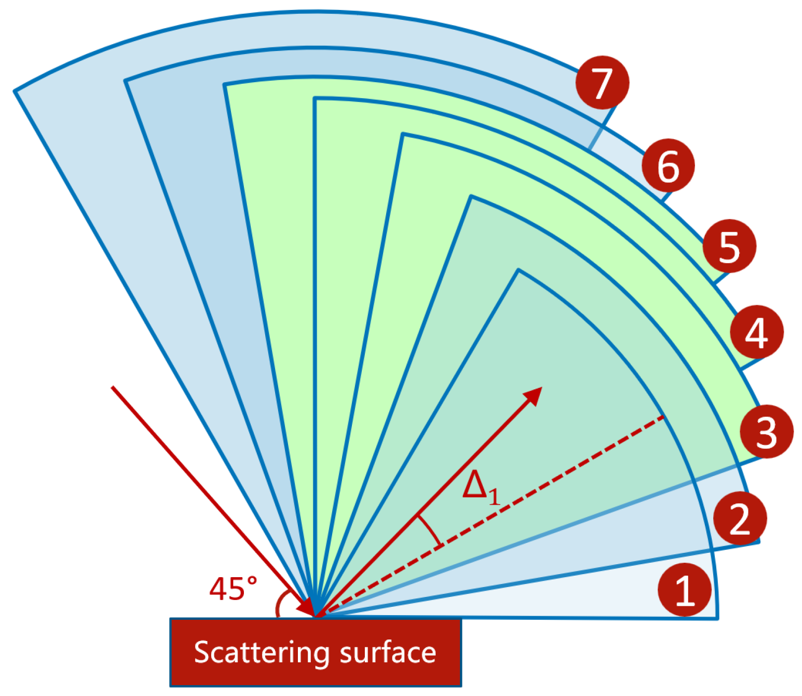
Narrow-angle window observation. We considered scenarios where collecting scattering data across a wide angular range is not feasible. In real-world settings, this may occur when building-obstructed wall surfaces are only accessible through a narrow angular window. It is important to evaluate the performance of our model under these angular constraints. We investigated a
angular window, striving to achieve effective recognition with a limited range of angles, as shown in
Figure 5. We also tried offsetting the angular window relative to the direction of specular reflection (with an offset angle
). The results are shown in
Table 4. We enforced a constraint of 20 scattering data points within each angle, which aligns with urban vehicle cruising speeds.
It should be noted that the best classification scores were achieved when the angular window enveloped the angles of mirror reflection and was slightly shifted towards the direction of richer features along the normal. Nevertheless, our method consistently achieved scores around 80%, even in the most angularly restrictive scenarios. This experiment demonstrates that our method can maintain high recognition accuracy at low angles, even under medium to low urban scanning speeds, further attesting to the validity of this approach.
7. Conclusions
In the field of integrated sensing and communication, environmental sensing is becoming as crucial as data transfer. This work proposes an approach in enhancing high-speed scanning capabilities for surface roughness recognition using terahertz frequency. Combining a deep learning framework, this method employs authentic high-speed sampling data to build an automated platform capable of capturing high-fidelity data in scenarios that closely emulate real-world dynamics. The manufacturing and 3D laser characterization of a spectrum of surfaces have facilitated the creation of a rich dataset, important for the training of our specialized neural network. We have aligned our emulated environments with actual laboratory and urban conditions, customizing our model to overcome three typical high-speed challenges: random occlusion, high-speed sparse data, and narrow-angle window observations.
Our experimental results have confirmed the effectiveness of this method, by achieving an score of over 95% in scenarios with random occlusion. This indicates exceptionally high accuracy within our current dataset, especially in relatively slower situations. Additionally, our approach consistently maintains scores above 90%, 80%, and 70% at emulated vehicular cruising speeds (40 km/h), urban vehicle speed limits (60 km/h), and drone flight speeds (80 km/h), respectively. Notably, we have achieved a 71% score within a range using only 10 randomly positioned scattering data points, highlighting the success of our method in challenging conditions. Moreover, we have identified window positions within a angular range that consistently maintain high speeds, resulting in scores above 90% with 20 randomly positioned scattering data points. This approach demonstrates exceptional accuracy, especially in medium- to low-speed scenarios and constrained angular windows. Even under extreme conditions, such as very high speeds (e.g., 80 km/h), it maintains a significant degree of reliability. This method may not only prompt the application of terahertz frequency band in surface recognition, but also enriches the broader context of sensing-communication integration, contributing to the evolution of intelligent, high-speed recognition systems.
For future works, we have two primary objectives: 1. We intend to deploy the methods presented in this paper onto actual vehicles, conducting real-world field experiments to validate and refine our approach. Our ultimate aim is to implement practical and effective scanning technologies with real-world applicability. 2. We plan to explore scenarios involving more complex scattering angles, such as surfaces with inclined incidence, Rx and Tx operating in different planes, to support applications in diverse and complex real-world environments.
Author Contributions
Methodology, J.L. and M.W.; Software, J.L. and Y.Q.; Validation, G.L. and C.Z.; Formal analysis, J.M.; Investigation, J.L. and J.M.; Resources, J.M.; Data curation, J.L. and D.L.; Writing—original draft, J.L.; Writing—review & editing, J.L.; Visualization, J.M.; Supervision, J.M.; Project administration, J.M.; Funding acquisition, J.M. All authors have read and agreed to the published version of the manuscript.
Funding
This work was supported in part by the National Natural Science Foundation of China (62071046) and the Science and Technology Innovation Program of Beijing Institute of Technology (2022CX01023).
Institutional Review Board Statement
This study did not involve any experiments on animals or humans.
Informed Consent Statement
Informed consent was not required for this study as it did not involve human participants.
Data Availability Statement
Data available within the article and available on request from the corresponding authors.
Conflicts of Interest
The authors declare no conflict of interest.
Appendix A. Surface Sample Characteristics
We characterized the surface roughness features based on high-precision point cloud data of the entire surface by the 3D laser scanning technique. Uniform sampling was performed and the calculation range was determined based on the illumination area. The RMS value was calculated based on the surface features within the calculation region.
Figure A1a–g display the RMS distributions of all seven surfaces. The horizontal and vertical axes represent the offset relative to the central point, and the heatmap values represent RMS values in millimeters (mm).
Figure A1h illustrates the effects of all seven surfaces simultaneously in a 3D schematic.
Figure A1.
The heatmaps for RMS values of each surface and the combined display of all seven surfaces in a 3D schematic.
Figure A1.
The heatmaps for RMS values of each surface and the combined display of all seven surfaces in a 3D schematic.
References
- Song, H.J.; Nagatsuma, T. Present and future of terahertz communications. IEEE Trans. Terahertz Sci. Technol. 2011, 1, 256–263. [Google Scholar] [CrossRef]
- Piesiewicz, R.; Jansen, C.; Mittleman, D.; Kleine-Ostmann, T.; Koch, M.; Kurner, T. Scattering analysis for the modeling of THz communication systems. IEEE Trans. Antennas Propag. 2007, 55, 3002–3009. [Google Scholar] [CrossRef]
- Zhang, C.; Yi, W.; Liu, Y.; Hanzo, L. Semi-Integrated-Sensing-and-Communication (Semi-ISaC): From OMA to NOMA. IEEE Trans. Commun. 2023, 71, 1878–1893. [Google Scholar] [CrossRef]
- Raza, A.; Ijaz, U.; Ishfaq, M.K.; Ahmad, S.; Liaqat, M.; Anwar, F.; Iqbal, A.; Sharif, M.S. Intelligent reflecting surface-assisted terahertz communication towards B5G and 6G: State-of-the-art. Microw. Opt. Technol. Lett. 2022, 64, 858–866. [Google Scholar] [CrossRef]
- Cheng, X.; Duan, D.; Gao, S.; Yang, L. Integrated sensing and communications (ISAC) for vehicular communication networks (VCN). IEEE Internet Things J. 2022, 9, 23441–23451. [Google Scholar] [CrossRef]
- Moldovan, A.; Ruder, M.A.; Akyildiz, I.F.; Gerstacker, W.H. LOS and NLOS channel modeling for terahertz wireless communication with scattered rays. In Proceedings of the 2014 IEEE Globecom Workshops (GC Wkshps), Austin, TX, USA, 8–12 December 2014; pp. 388–392. [Google Scholar] [CrossRef]
- Sheikh, F.; Gao, Y.; Kaiser, T. A study of diffuse scattering in massive MIMO channels at terahertz frequencies. IEEE Trans. Antennas Propag. 2019, 68, 997–1008. [Google Scholar] [CrossRef]
- Ortolani, M.; Lee, J.; Schade, U.; Hübers, H.W. Surface roughness effects on the terahertz reflectance of pure explosive materials. Appl. Phys. Lett. 2008, 93, 081906. [Google Scholar] [CrossRef]
- Sabery, S.M.; Bystrov, A.; Gardner, P.; Stroescu, A.; Gashinova, M. Road surface classification based on radar imaging using convolutional neural network. IEEE Sens. J. 2021, 21, 18725–18732. [Google Scholar] [CrossRef]
- Ma, J.; Shrestha, R.; Moeller, L.; Mittleman, D.M. Invited Article: Channel performance for indoor and outdoor terahertz wireless links. APL Photonics 2018, 3, 051601. [Google Scholar] [CrossRef]
- Bystrov, A.; Hoare, E.; Gashinova, M.; Cherniakov, M.; Tran, T.Y. Experimental study of rough surface backscattering for low terahertz automotive radar. In Proceedings of the 2019 20th International Radar Symposium (IRS), Ulm, Germany, 26–28 June 2019; pp. 1–7. [Google Scholar] [CrossRef]
- Taleb, F.; Hernandez-Cardoso, G.G.; Castro-Camus, E.; Koch, M. Transmission, Reflection, and Scattering Characterization of Building Materials for Indoor THz Communications. IEEE Trans. Terahertz Sci. Technol. 2023, 13, 421–430. [Google Scholar] [CrossRef]
- Jansen, C.; Priebe, S.; Moller, C.; Jacob, M.; Dierke, H.; Koch, M.; Kurner, T. Diffuse scattering from rough surfaces in THz communication channels. IEEE Trans. Terahertz Sci. Technol. 2011, 1, 462–472. [Google Scholar] [CrossRef]
- Sheikh, F.; Zantah, Y.; Mabrouk, I.B.; Alissa, M.; Barowski, J.; Rolfes, I.; Kaiser, T. Scattering and roughness analysis of indoor materials at frequencies from 750 GHz to 1.1 THz. IEEE Trans. Antennas Propag. 2021, 69, 7820–7829. [Google Scholar] [CrossRef]
- Fukuchi, T.; Fuse, N.; Mizuno, M.; Fukunaga, K. Surface roughness measurement using terahertz waves. In Proceedings of the 3rd International Conference on Industrial Application Engineering, Hiroshima, Japan, 17–19 April 2015; pp. 294–299. [Google Scholar] [CrossRef]
- Schecklman, S.; Zurk, L.M.; Henry, S.; Kniffin, G.P. Terahertz material detection from diffuse surface scattering. J. Appl. Phys. 2011, 109, 094902. [Google Scholar] [CrossRef]
- Yi, H.; Guan, K.; Mathiopoulos, P.T.; Xie, P.; He, D.; Dou, J.; Zhong, Z. Full-Wave Simulation and Scattering Modeling for Terahertz Communications. IEEE J. Sel. Top. Signal Process. 2023, 17, 713–728. [Google Scholar] [CrossRef]
- Sabery, S.M.; Bystrov, A.; Navarro-Cía, M.; Gardner, P.; Gashinova, M. Study of low terahertz radar signal backscattering for surface identification. Sensors 2021, 21, 2954. [Google Scholar] [CrossRef] [PubMed]
- Stroescu, A.; Cherniakov, M.; Gashinova, M. Classification of high resolution automotive radar imagery for autonomous driving based on deep neural networks. In Proceedings of the 2019 20th International Radar Symposium (IRS), Ulm, Germany, 26–28 June 2019; pp. 1–10. [Google Scholar] [CrossRef]
- Buch, N.; Velastin, S.A.; Orwell, J. A review of computer vision techniques for the analysis of urban traffic. IEEE Trans. Intell. Transp. Syst. 2011, 12, 920–939. [Google Scholar] [CrossRef]
- Cooper, C.; Zhang, J.; Hu, L.; Guo, Y.; Gao, R.X. Texture-Aware Ridgelet Transform and Machine Learning for Surface Roughness Prediction. IEEE Trans. Instrum. Meas. 2022, 71, 2520110. [Google Scholar] [CrossRef]
- Singh, A.; Gaurav, K.; Rai, A.K.; Beg, Z. Machine learning to estimate surface roughness from satellite images. Remote Sens. 2021, 13, 3794. [Google Scholar] [CrossRef]
- Valikhani, A.; Jaberi Jahromi, A.; Pouyanfar, S.; Mantawy, I.M.; Azizinamini, A. Machine learning and image processing approaches for estimating concrete surface roughness using basic cameras. Comput.-Aided Civ. Infrastruct. Eng. 2021, 36, 213–226. [Google Scholar] [CrossRef]
- Zeng, Y.; Ma, Y.; Sun, S. Joint radar-communication: Low complexity algorithm and self-interference cancellation. In Proceedings of the 2018 IEEE Global Communications Conference (GLOBECOM), Abu Dhabi, United Arab Emirates, 9–13 December 2018; pp. 1–7. [Google Scholar] [CrossRef]
- Zhang, Y.; Wang, Q.; Qin, H.; Meng, J. Adaptive self-interference cancellation system for microwave LFMCW radar with optimal delay matching. In Proceedings of the 2019 Joint International Symposium on Electromagnetic Compatibility, Sapporo and Asia-Pacific International Symposium on Electromagnetic Compatibility (EMC Sapporo/APEMC), Sapporo, Japan, 3–7 June 2019; pp. 729–732. [Google Scholar] [CrossRef]
- Ma, J.; Shrestha, R.; Zhang, W.; Moeller, L.; Mittleman, D.M. Terahertz wireless links using diffuse scattering from rough surfaces. IEEE Trans. Terahertz Sci. Technol. 2019, 9, 463–470. [Google Scholar] [CrossRef]
- Degli-Esposti, V.; Fuschini, F.; Vitucci, E.M.; Falciasecca, G. Measurement and modelling of scattering from buildings. IEEE Trans. Antennas Propag. 2007, 55, 143–153. [Google Scholar] [CrossRef]
- Ulaby, F.; Moore, R.; Fung, A. Microwave Remote Sensing: Active and Passive. Volume 2-Radar Remote Sensing and Surface Scattering and Emission Theory; Artech House Inc.: Norwood, MA, USA, 1982. [Google Scholar]
- Hochreiter, S.; Schmidhuber, J. Long Short-Term Memory. Neural Comput. 1997, 9, 1735–1780. [Google Scholar] [CrossRef] [PubMed]
- Srivastava, N.; Hinton, G.; Krizhevsky, A.; Sutskever, I.; Salakhutdinov, R. Dropout: A simple way to prevent neural networks from overfitting. J. Mach. Learn. Res. 2014, 15, 1929–1958. [Google Scholar]
- Kingma, D.P.; Ba, J. Adam: A method for stochastic optimization. arXiv 2014, arXiv:1412.6980. [Google Scholar] [CrossRef]
- Taha, A.A.; Hanbury, A. Metrics for evaluating 3D medical image segmentation: Analysis, selection, and tool. BMC Med. Imaging 2015, 15, 29. [Google Scholar] [CrossRef]
- Yu, J.; Zhu, H.; Han, H.; Chen, Y.J.; Yang, J.; Zhu, Y.; Chen, Z.; Xue, G.; Li, M. Senspeed: Sensing driving conditions to estimate vehicle speed in urban environments. IEEE Trans. Mob. Comput. 2015, 15, 202–216. [Google Scholar] [CrossRef]
| Disclaimer/Publisher’s Note: The statements, opinions and data contained in all publications are solely those of the individual author(s) and contributor(s) and not of MDPI and/or the editor(s). MDPI and/or the editor(s) disclaim responsibility for any injury to people or property resulting from any ideas, methods, instructions or products referred to in the content. |
© 2024 by the authors. Licensee MDPI, Basel, Switzerland. This article is an open access article distributed under the terms and conditions of the Creative Commons Attribution (CC BY) license (https://creativecommons.org/licenses/by/4.0/).


 ,
, 
