Article

Research on Defect Detection Method for Composite Materials Based on Deep Learning Networks

1
School of Computer Science and Engineering, Xi’an Technological University, Xi’an 710016, China
2
School of Software, Northwestern Polytechnical University, Xi’an 710129, China
*
Author to whom correspondence should be addressed.
Appl. Sci. 2024, 14(10), 4161; https://doi.org/10.3390/app14104161
Submission received: 26 February 2024 / Revised: 10 May 2024 / Accepted: 12 May 2024 / Published: 14 May 2024

Abstract

:
Compared to traditional industrial materials, composites have higher durability and compressive strength. However, some components may have flaws due to the manufacturing process. Traditional defect detection methods have low accuracy and cannot adapt to complex shooting environments. Aiming to address the issues of high computational requirements in traditional detection models and the lack of lightweight detection capabilities, the Ghost module is used instead of convolutional arithmetic to construct a lightweight model. To reduce the computational complexity of the feature extraction module, we have incorporated an improved Efficient Channel Attention mechanism to improve the model’s feature extraction capabilities. A rapid defect classification method is implemented to determine whether there are defects in the image or not by comparing the performance and running speed of models such as AlexNet, VGGNet, and ResNet. And ablation experiments are conducted for each model. The results show that the Ghost module model, which incorporates the improved Efficient Channel Attention mechanism, has a significant optimization effect on the convolutional neural network model. It can achieve a high accuracy rate when constructing lightweight models. It improves the running speed of the model, making it more efficient to use and deploy.

1. Introduction

Composite materials commonly exhibit various defects during the production process, often requiring the use of X-rays or other imaging tools to assess their shape. To enhance the efficiency and accuracy of defect detection in composite materials, computer vision algorithms that employ conventional image processing techniques are utilized.
In considering the visual characteristics of defects in traditional industrial materials, defect detection can be classified into two types: linear defects and nonlinear defects. For linear features, detection algorithms such as the Hough transform [1] for straight lines and edge operator detection [2] are used. The Hough transform extracts straight line features in an image but requires manual parameterization. Different parameters can affect the number of straight lines detected. The edge operator is easily influenced by the internal texture information of the image, which can lead to the detection of more invalid information. Nonlinear features utilize threshold segmentation algorithms, level-set algorithms, and morphological algorithms [3,4,5]. The threshold segmentation algorithm has a limited range of applicability. The level-set algorithm is suitable for all kinds of complex situations, but it requires finding the initial point where the diffusion begins first. Morphology algorithms are more effective for detecting small targets but are generally less effective for detecting targets in the edge region of the image. To address the complexity of defect features, various methods can be employed, including the hybrid Gaussian model, superpixel segmentation, and grayscale covariance matrix [6,7,8]. These methods can detect various irregularly shaped defects, although they are limited to detecting only one specific type of defect.
Defect detection algorithms based on deep learning network models can overcome the shortcomings of traditional algorithms and adapt to various application scenarios [9,10,11,12]. Commonly used methods include image classification, target detection tasks, and semantic segmentation tasks [13]. Convolutional neural networks (CNNs) have been improved and are now utilized in various defect detection applications [14,15]. T. Wang et al. constructed a multilayer convolutional neural network using the traditional CNN structure and utilized the concept of separate detection for the multi-classification of various defects in a dataset [16]. In the task of surface defect detection in industrial concrete, Suh et al. utilized the Faster R-CNN target detection network for industry-specific detection and achieved improved detection results [17]. Deep learning-based methods effectively overcome challenges in detecting composite defects and demonstrate better adaptability to complex application scenarios, ensuring more accurate defect detection in composite materials [18,19,20].
This study focuses on various types of defects in composite materials, analyzing both semantic and morphological data. It analyzes the characteristics of semantic distribution in composite material images and principles for capturing different components. Combining traditional computer vision algorithms, the dataset for defect detection in composite materials is obtained through preprocessing. A fast classification model has been developed using a deep learning network to enhance efficiency and accuracy. The main research content of this paper includes the following:
(1)
We designed a lightweight and highly accurate model for rapidly classifying defects in composite images. The Ghost module extracts features from the input image, calculating a reduced number of parameters. The module utilizes feature map redundancy by employing convolutional operations to generate a segment of the feature map. This is then followed by linear operations to duplicate and enlarge the feature map, thereby reducing the computational load.
(2)
We introduce and improve the Efficient Channel Attention (ECA) mechanism. By incorporating the ECA module into the feature extraction process, distinct weights are assigned to each channel of the feature map. The channel-based attention mechanism enhances the accuracy of the model in pattern recognition.
The remainder of this paper is structured as follows: In the second part, we present the structure of the deep learning network for images and the attention mechanism module. In the third part, a rapid classification method for composite defects is proposed. The fourth part describes experimental tests and an analysis of the obtained results. The fifth part provides a summary of the entire paper.

2. Related Works

2.1. Convolutional Neural Network Architecture

The convolutional layer is a crucial component of a CNN, incorporating two essential characteristics: the local receptive field and weight sharing. The network architecture serves the purpose of extracting and analyzing feature information from images and mapping it to a higher-dimensional space. Convolutional operations involve important parameters such as the number, size, stride, and padding method. These parameters determine the behavior of the convolutional layer. Apart from standard convolution operations, there are variations such as deep convolution and one-dimensional convolution. The downsampling layer, also known as the pooling layer, is primarily used after convolution to reduce the number of parameters in the feature map and prevent overfitting. Simultaneously, pooling operations enlarge the model’s receptive field, extracting more comprehensive semantic information.
Conversely, the upsampling layer increases image resolution through the process of deconvolution. Unlike downsampling, which reduces the size of an image, inverse convolution increases the image size by mapping low-resolution features to high resolution. The Fully Connected Layer (FC), typically positioned at the end of the CNN, adjusts the number of output nodes based on the desired number specified by the model. The weight matrix implements the connection weights for the FC, encapsulating the calculated values. These weights determine the final output of the node by passing through an activation function.
In the structure of a neural network, convolution, upsampling/downsampling, and FC are linear operations. However, a challenge arises in deep learning models when linear mappings fail to capture nonlinear relationships. To address this, an activation function is incorporated at the end of each layer, transforming the model from linear to nonlinear mapping. This inclusion empowers the network with the ability to fit nonlinear functions.

2.2. Attention Mechanisms

The attention mechanism is a prominent feature in the feature extraction stage of the model, particularly within the convolutional component. The function of the model allows it to prioritize regions that contain a significant amount of semantic information, thereby enhancing classification accuracy. Attention mechanisms can be broadly classified into spatial attention mechanisms and channel attention mechanisms, each adhering to distinct principles.
The channel attention mechanism enhances the attention weights of the model at the channel level, assigning different weights to each channel in the feature map data. Channels deemed crucial for achieving accurate results carry greater significance. Notable channel attention mechanisms include the SE attention mechanism [21] and the enhanced ECA mechanism [22]. The SE attention mechanism consists of two crucial steps: the S (squeeze) part and the E (excitation) part. The squeeze operation manipulates the global receptive field of the feature map, while the excitation operation computes weight values for each channel. The ECA mechanism simplifies the process of assigning channel weights from SE by replacing the two FC with a one-dimensional convolution (Conv1d). This results in weight data of the same size. The key distinction lies in the ECA mechanism, which utilizes a one-dimensional convolution and produces channel weights using the sigmoid activation function.
The spatial attention mechanism, in contrast, operates on the target’s location information within the feature map. It assigns varying weights to data at each position in the feature map, enhancing the model’s ability to identify the target and placing greater emphasis on the target object’s location within the image. This, in turn, improves the accuracy of recognition. A well-known spatial attention mechanism is the Spatial Attention Module (SAM), which is integrated as part of the Convolutional Block Attention Module [23].

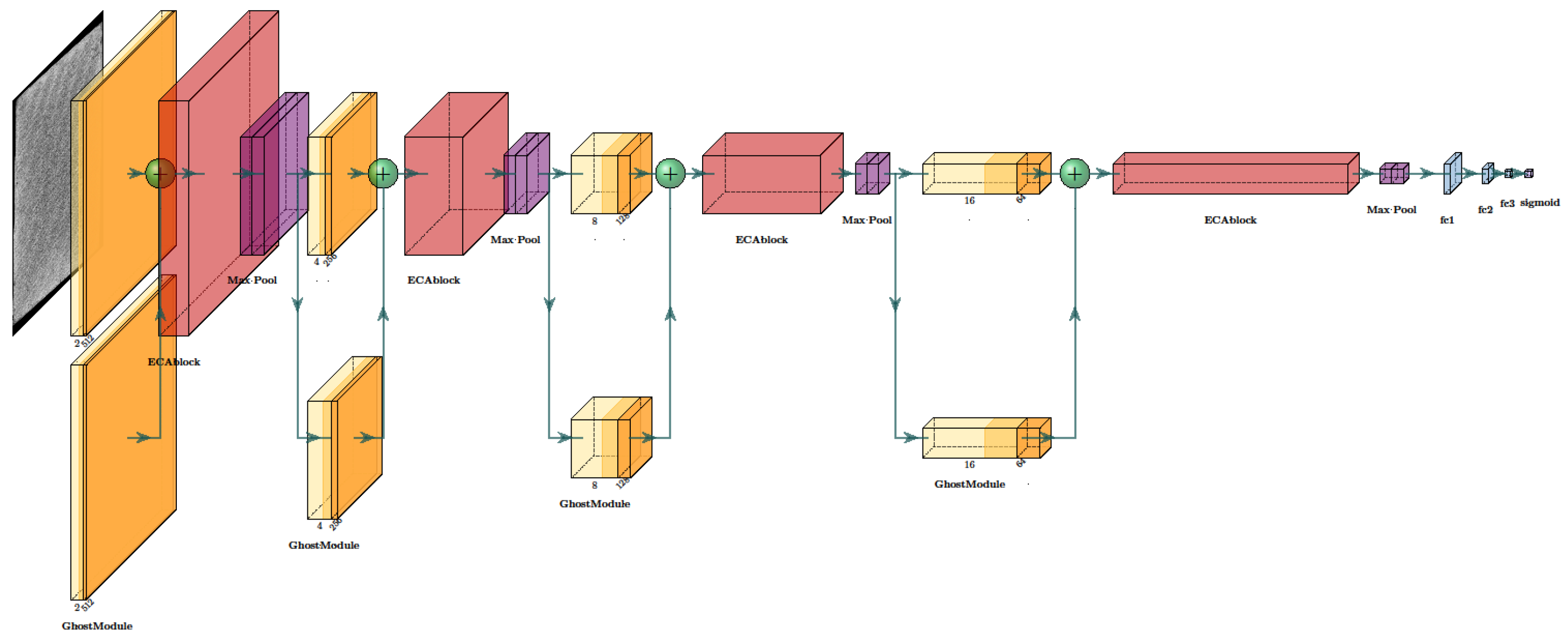
3. ECA Ghost CNN Method
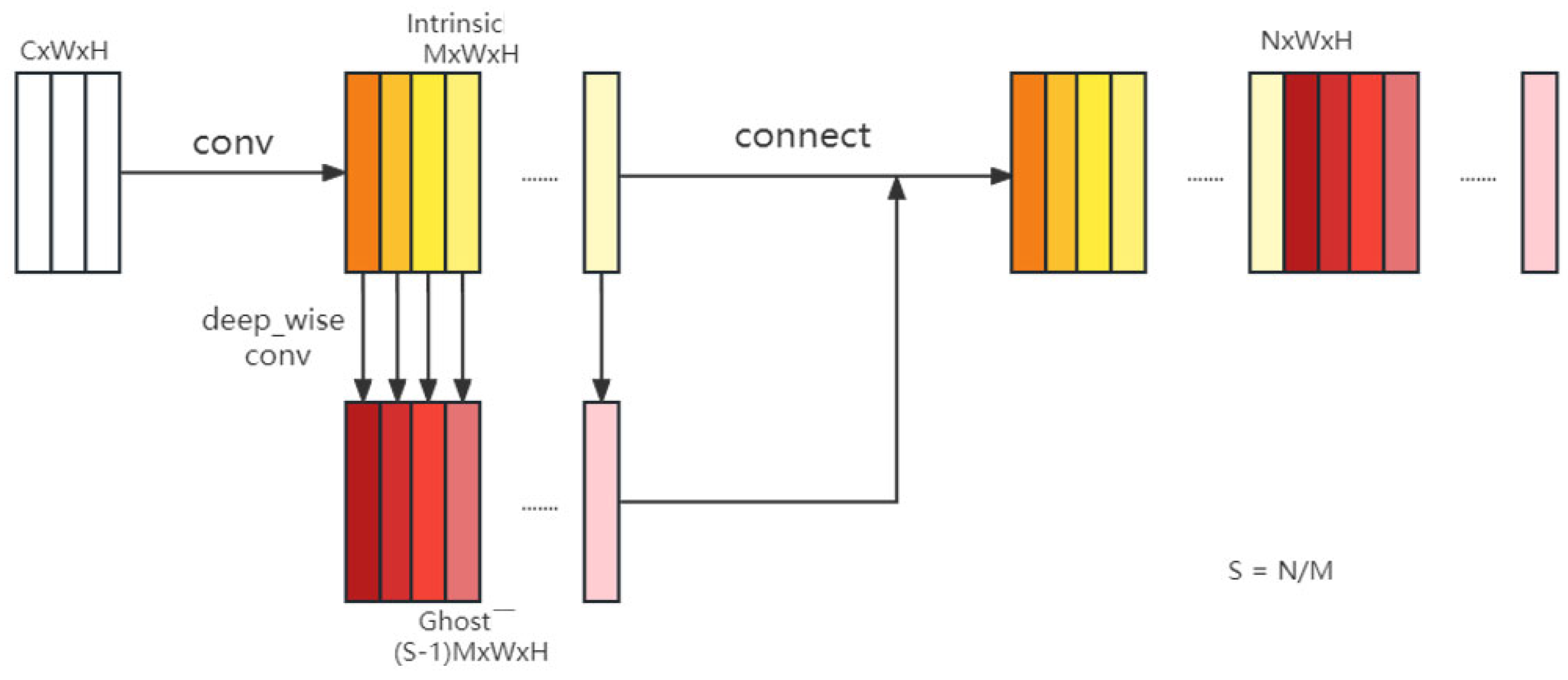
The improved ECA mechanism Ghost module model is abbreviated as ECAGhostCNN. The overall structure of the rapid classification model for composite material defects is depicted in Figure 1. The entire model undergoes four rounds of feature extraction, introducing the Ghost module to replace traditional convolutional (conv) operations for a more efficient implementation of the model. Additionally, an enhanced ECA mechanism module is incorporated during the feature extraction process to improve the performance of the model. Each round of feature extraction begins with a layer based on the Ghost module with the ECA mechanism, followed by a layer using the Ghost module without ECA. Finally, three FCs are applied, with the first two utilizing the ReLU activation function, and the last one using the sigmoid activation function. This results in a final prediction of size 1 × 1 × 1 . The final output represents the binary classification result of whether a defect is present in the image.
The entire classification network model is based on a traditional CNN, which consists of feature extraction structures, pooling structures, attention modules, and an FC. Two rounds of feature extraction, followed by pooling, are performed consecutively. The model’s prediction is obtained from the final FC. In this study, two Ghost modules are used for each feature extraction, and the number of output channels increases in the first iteration. The Ghost module helps save a significant amount of computational resources. In the second round, the channel count remains unchanged, and an attention mechanism is added on top of the Ghost module. This allows the model to prioritize the feature information in the original image.
The detection results of the ECAGhostCNN model are shown in Figure 1 below.
The input dimension is a raw image with dimensions of 1 × 512 × 512 . After being transformed by the ECAGhostCNN model, the final output values range from 0 to 1. If the value is greater than 0.5, the component is considered to have a defect; otherwise, it is considered normal.

3.1. Ghost Module

The structure of the Ghost module is shown in Figure 2. Its main idea is to leverage the redundancy in feature maps during the convolution process. The Ghost module initially performs a small number of convolutions to obtain a certain quantity of feature maps. Then, instead of convolution operations, it applies linear operations to each feature map under each channel, generating a set of ghost feature maps in relation to the intrinsic feature map. Subsequently, the ghost feature maps are concatenated with the intrinsic feature map to obtain the final feature map.
In the figure, S represents the quotient of the final output feature map channel quantity and the number of intrinsic maps. M is the final output feature map channel quantity, and N is the number of intrinsic maps.
The depth-wise convolution of the intrinsic map divides the convolution process into two steps. Unlike regular convolution, depth-wise convolution determines the number of convolutional operation kernels in the first step based on the number of input feature map channels. Each convolutional kernel is responsible for operating on a specific channel’s feature map, mapping the data from that channel’s feature map to the resulting output after the convolution operation. Therefore, the output channel quantity of the first step in depth-wise convolution is the same as the input data channel quantity.
Next, a regular convolution operation is performed using a 1 × 1 kernel to obtain a new feature map. The use of a 1 × 1 kernel significantly reduces computational complexity during the operation. Depth-wise convolution, compared to regular convolution, reduces the computational operations of the convolutional kernel on each channel, thereby decreasing the number of parameters required for computation.
The compression ratio can be used to measure the number of parameters saved by the Ghost module compared to a standard convolution module. It is defined as the ratio of the number of parameters operated by the original convolution to the number of parameters operated by the current module. The specific formula is as follows:
r c = n × c × k × k n s × c × k × k + s 1 × n s × d × d
where “ c ” represents the number of input channels in the Ghost module, and “ n ” represents the number of output channels in the module. “ k ” represents the size of the convolutional kernel in the first convolution operation of the Ghost module, i.e., k × k . “ d ” represents the size of the convolutional kernel used in the depth-wise convolution process, i.e., d × d . “ s ” represents the quotient of the number of output channels (“ n ”) and the number of channels (“ m ”) after the first convolution step, which can be calculated as s = n / m . Through approximate calculations, it can be determined that using the Ghost module can achieve a compression ratio of approximately s in terms of parameter reduction. In the model design, this paper sets the value of k as 5 and the value of d as 3. The value of “ s ” in the Ghost module operation is determined by the number of output channels obtained from the first convolution of the module. In this case, s is set to 8, which means that after the first convolution in the Ghost module, each channel generates 7 ghost maps and 1 original map through depth-wise convolution. Experimental results show that the addition of the Ghost module significantly reduces the parameters of the feature extraction layers in the model. Except for the compression ratio of the first Ghost module, the compression ratios of the other modules are close to the initially set value of s . This improvement in parameter reduction enhances the computational speed of the model while maintaining its performance.

3.2. Efficient Channel Attention Module

In this paper, the global pooling operation in the ECA mechanism has been improved, and the model has been optimized using the improved ECA mechanism. The ECA block replaces the attention computation module based on the SE block. It requires fewer parameter computations and better aligns with the requirements of lightweight model design.
The attention mechanism module in SE is used to optimize the CNN. The convolution operation in the CNN enables the integration of spatial and channel information within the local receptive field of each layer. This process leads to the generation of meaningful features.
In the ECA block, the structure performs pooling of feature maps within each channel. Average pooling is commonly used to preserve the background information in the image on a global scale. Max pooling is used to capture extreme values and preserve texture information in the image since the background in the image of the composite material contains more semantic information, while the defects are visible in the texture information of the components. Therefore, in this paper, the global pooling operation in ECA is improved by using a pooling method that combines average pooling and maximum pooling. The specific principle is shown in Figure 3. Compared to the original ECA block, the addition of the influence of feature values from both average pooling and max pooling helps to prevent the omission of finer-grained features.
In the improved ECA module, the feature maps undergo both mean pooling and max pooling separately. This process extracts information from each channel of the feature map, resulting in data of size 1 × 1 × C . The two results are then added channel-wise while maintaining the original size. Subsequently, the obtained data undergo one-dimensional convolution, and the sigmoid activation function is applied to obtain attention weights for each channel. During the one-dimensional convolution process, the ECA block focuses more on the relationships between adjacent channels in the feature map. A one-dimensional convolution with a kernel size of k is applied between adjacent channels to facilitate cross-channel interactions, thus avoiding dimension reduction operations, as observed in the SE block. ECA employs a frequency band matrix, W k , to facilitate the exchange of information between channels, thereby ensuring efficient and effective information extraction. The frequency band matrix is illustrated below.
w 1,1 w 1 , k 0 0 0 0 w 2,2 w 2 , k + 1 0 0 0 0 0 w C , C k + 1 w C , C
Each row in the matrix contains k values of the non-constant number 0, which represents the k channels surrounding each channel involved in the relational operation. C represents the number of channels. In general, C is an integer that is a power of 2. The entire matrix involves a total of k × C parameters. When participating in the computation, each channel only operates with its k adjacent channel neighbors. The operation can be achieved by using a one-dimensional convolution with a kernel size of 1 × k . It is possible to share the learning parameters among the channels, thereby improving performance. This approach is known as ECA-NS.
The ECA block can be obtained by replacing the FC of the MLP structure in the SE block with the one-dimensional convolution of the ECA-NS method. It can be directly attached to the feature extraction component of the model to enhance its performance. Meanwhile, compared to the SE block, the ECA block has fewer parameters, which can improve the model’s running speed.

3.3. Fully Connected Layer and Loss Function

There are three FCs in the final output section of the model. The final feature extracted by the Ghost module results in a feature map size of 8 × 8 × 1024. The outputs of the first two FCs are 1024 and 512, respectively. The activation function uses the ReLU activation function. The last layer has an input size of 1, representing the predicted category of the image, and utilizes the sigmoid activation function.
The sigmoid activation function normalizes the output of the neuron and maps it to the interval between 0 and 1. In binary image classification, the output can be classified as binary with the predicted value constrained to be 0.5 as a cut-off. The sigmoid function has the following expression:
σ x = 1 1 + e x
The sigmoid function converges to a smooth state as the input variables approach positive or negative infinity. The more the function approaches positive infinity, the more the value approaches 1. Similarly, as the function approaches negative infinity, the value approaches 0. In the binary classification problem, the output value range of the sigmoid function can be utilized to represent the binary prediction result of the model.
The model uses the binary_crossentropy loss function to assess the accuracy of the classification. The expression for this function is shown below:
E = y i log   ( p ( y i ) ) + ( 1 y i ) log   ( 1 p ( y i ) )
where y i represents the label value of the image in the training set. Since it is a binary classification problem, the value of y i is denoted as either 0 or 1, representing the two categories to be classified. p ( y i ) is the predicted value of the model output, i.e., the output of the sigmoid function from the last FC. In a binary classification problem, when the label value of an image is 1, the value of 1 y i is 0. Consequently, the predicted value p ( y i ) of the image tends to approach 1. Taking the logarithm of this value reduces it towards 0, resulting in a smaller loss function value. During the training process, the model’s predictions gradually converge towards 1. Conversely, when the label value of the image is 0, y i is also 0. In this case, as the predicted value p ( y i ) of the image approaches 0, the value of 1 p ( y i ) approaches 1. When taking the logarithm, the value tends to approach 0, resulting in a smaller loss function value. By utilizing the binary_crossentropy function, the model can be effectively trained to perform binary classification tasks.

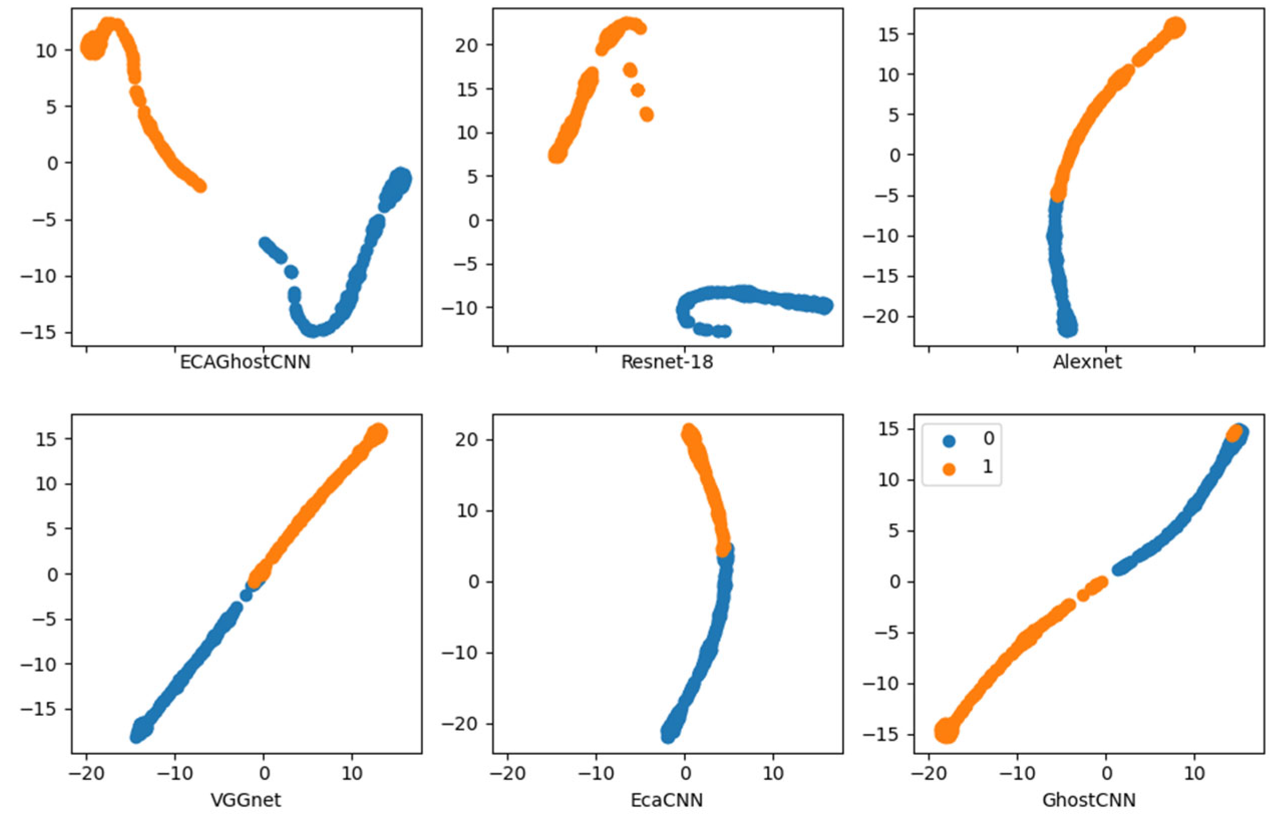
4. Results and Discussion
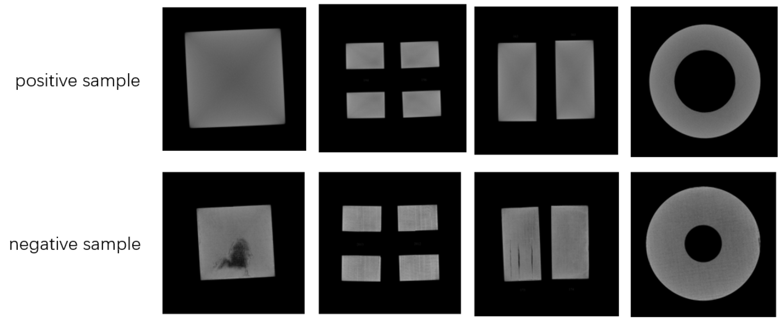
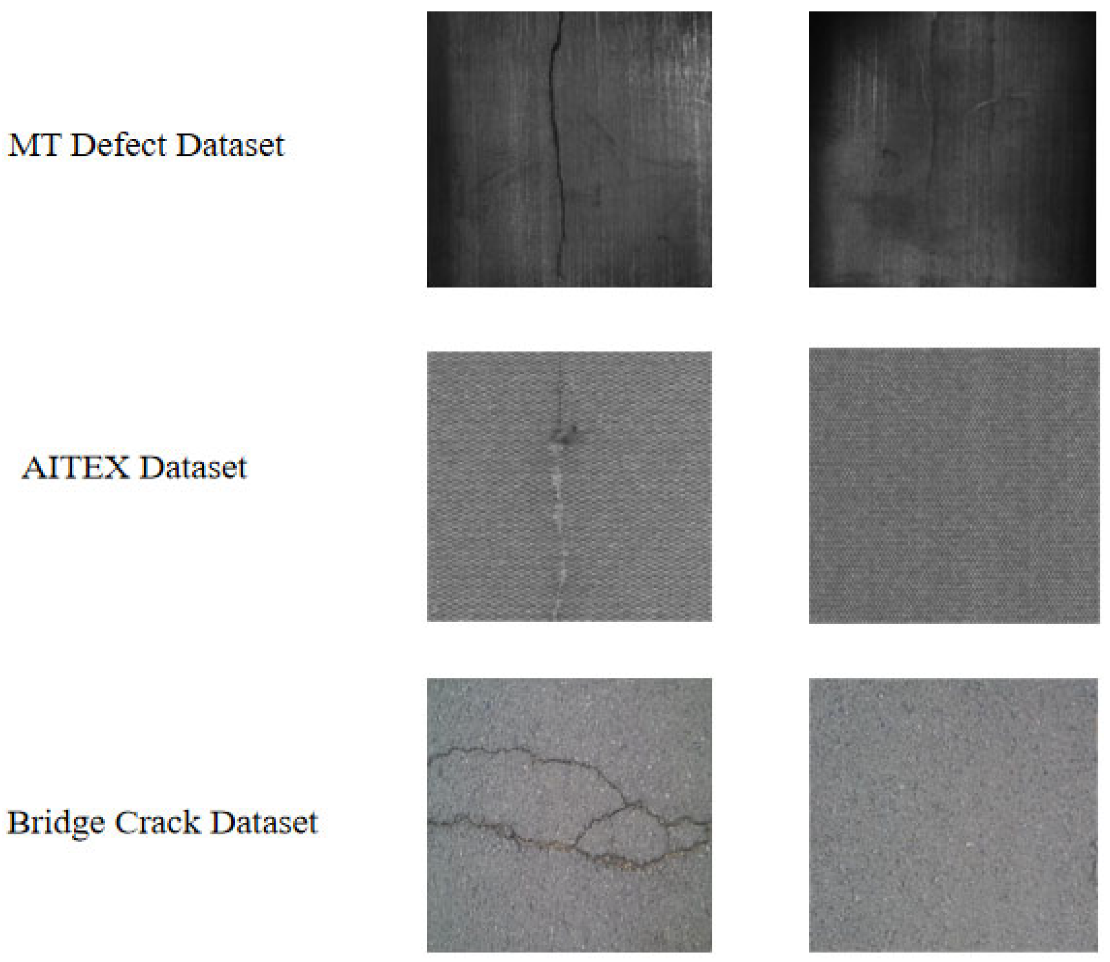
4.1. Datasets

The dataset is expanded here due to the limited amount of original composite data. The expanded section utilizes the steel dataset from Northeastern University, which shows a significant similarity to the composite image features. The composite material image dataset is derived from the CT scanning process of an industrial production company. The dataset consists of a total of 266 images. The steel dataset was selected to obtain 500 images, while the entire dataset consists of a total of 766 images. This includes both positive samples with defects and negative samples without defects, as shown in Figure 4. The size of the dataset images is 2048 × 2048. After preprocessing, which includes denoising and feature enhancement, the image size is reduced to 512 × 512. The images are all single-channel, 8-bit grayscale images. During processing, the dataset is divided into 606 sheets for the training set and 160 sheets for the testing and validation sets. The training set is used to train the model. The validation set is used to compare and evaluate the performance of the model.
In order to validate the scalability of the classification model based on the Attention Ghost module, in this paper, the model’s performance is tested using datasets from various industrial domains. These include the MT Defect Dataset [24], the AITEX Dataset, and the Bridge Crack Dataset [25,26]. The three datasets record material defect data from various industrial domains. The MT Defect Dataset includes six different types of surface defects on tiles. From the MT Defect Dataset, 400 images of both positive and negative samples are selected in this paper. Among them, 60 images of positive and negative samples are randomly selected for the test set, while the remaining images are used for the training set. The Bridge Crack Dataset focuses on crack detection and showcases various surface features and crack patterns. From the AITEX Dataset and the Bridge Crack Dataset, 80 images with positive and negative samples are selected as the training set, while 20 images with positive and negative samples each are used as the test set in this paper, respectively. The positive and negative samples in the dataset are shown in Figure 5.

4.2. Comparison of Experimental Results

Figure 6 displays the predicted output values for all models on the test set. The output values range from 0 to 1. It can be observed that the predicted values from ECAGhostCNN and Resnet-18 are relatively scattered, indicating a clear and meaningful distinction. In contrast, the predicted value distributions obtained by other algorithms, such as AlexNet, are not as distinct. There are overlapping predicted values, which indicate less precise predictions.
During the experiments, a binary cross-entropy loss function was used for each model. The initial learning rate was 0.001 and the Adam optimizer was used for model training with a training batch size of 20. The final performance of each model on the validation set (160 images in total) is shown in the Table 1.
It can be observed that the introduction of the attention mechanism has resulted in a significant improvement in the performance of the classification model on the composite dataset in this paper.
The F1 score [30] metric is used to evaluate the classification performance of the model. In the presence of an imbalance between positive and negative samples, the results indicate that the model utilized in this paper greatly enhances the classification performance.
In a standardized hardware and software environment, the running time of each model is compared individually for every sample in the test set. The results show that the running time of each image fluctuates. But, in general, the model based on the improved ECAGhost module has a relatively faster runtime than the other models. The average run time per image in the same environment is used to indicate the average speed at which the models operate. The comparison of the run speed of each model is shown in the Table 2.
It can be seen that the average running speed of the ECAGhostCNN model is faster than that of other models. The other models obviously have more arithmetic operations and a longer running time. This shows that the Ghost module plays a significant role in reducing the weight of the model and improving its operational efficiency.
After conducting experimental analysis, each specific value in the model is presented in the Table 3.
From the above data, it can be observed that the ECAGhostCNN model has an FLOPs value of 110.56 M, with 2,108,179 parameters, and it occupies 24.37 MB of memory. It can be seen that the ECAGhostCNN model, which incorporates the Ghost module and ECA module, has improved accuracy. While enhancing processing speed, it also ensures classification accuracy, making it valuable for practical applications.
This article presents a statistical analysis of the classification accuracy and average processing time per image for the model across various industrial datasets. The results indicate that the classification performance of the attention-based Ghost module is consistently stable across different datasets. It demonstrates superior accuracy and processing speed on diverse industrial datasets, making it well suited for rapid classification tasks involving industrial material images. This suggests that the model exhibits a certain level of scalability in industrial material applications.
To validate the performance improvement and speed enhancement of the model after incorporating the Ghost module and an improved ECA mechanism, ablation experiments were conducted in this study. A comparison was made with models proposed in datasets from various industrial domains. The results are shown in the Table 4.
From the experimental results, it is evident that the ECACNN model achieved a 17.50% increase in accuracy compared to the CNN model, albeit with a decrease in runtime speed. The MCuePushU model achieved an accuracy as high as 98.52%, but with a runtime speed of 549 ms. Meanwhile, both the deepCrack and Unet models exhibited significantly slower runtime speeds compared to the ECAGhostCNN model’s 10.53 ms. This may be attributed to the fact that MCuePushU and deepCrack are extensions of Unet, which have a large number of parameters that require more computation time. The GhostCNN model demonstrated a speed improvement of 9.91 ms over the CNN model, with little change in classification accuracy.
The results indicate that the ECA module can enhance the model’s focus on semantic information in the images, thereby improving the model’s accuracy. The Ghost module can reduce parameter calculations, improve operational efficiency, and facilitate lightweight deployment of the model. The attentional Ghost module proposed in this paper has a significant optimization effect on the CNN model. It can achieve high accuracy while building lightweight models, enhancing model runtime speed, and facilitating model usage and deployment.

5. Conclusions

In this paper, we investigate the problem of efficiently classifying defects in composite materials. We propose a non-destructive defect detection method based on deep learning for analyzing composite images. The composite defect detection dataset is constructed by preprocessing the raw data to address various types of issues. The ECAGhostCNN lightweight model, which is designed based on the Attention Ghost module, is introduced. The Ghost module leverages the redundancy of the output feature maps in the convolutional layer to decrease its computational workload. ECA utilizes the operation of assigning weights to the channels of the feature map to enhance the model’s focus on the regions that are defective. After comparing each model, ablation experiments were conducted on each of them. CNN, ECACNN, GhostCNN, and ECAGhostCNN were compared. Finally, the construction of a CNN model based on the Attention Ghost module was completed. The rapid classification of composite materials was achieved. The accuracy of pixel detection and the speed of classification were significantly improved.

Author Contributions

Conceptualization, J.C., W.T. and Y.Y.; methodology, J.C.; software, J.C.; validation, W.T., Y.Y. and Z.Z.; formal analysis, Z.Z. and Y.C.; investigation, W.T.; resources, J.C.; data curation, Y.C.; writing—original draft, Y.C.; writing—review and editing, J.C. and W.T.; supervision, Y.Y.; visualization, Z.Z. All authors have read and agreed to the published version of the manuscript.

Funding

Shaanxi Province Key R&D Program General Project-Industrial Field (No. 2024GX-YBXM-139); Aviation Science Foundation (No. 20185853038, No. 201907053004); Shanghai Aerospace Science and Technology Innovation Fund (No. SAST2021-054).

Institutional Review Board Statement

Not applicable.

Informed Consent Statement

Not applicable.

Data Availability Statement

The data in this article are available from the corresponding author.

Conflicts of Interest

The authors declare no conflicts of interest.

References

  1. Mochizuki, Y.; Torii, A.; Imiya, A. N-Point Hough transform for line detection. J. Vis. Commun. Image Represent. 2009, 20, 242–253. [Google Scholar] [CrossRef]
  2. Bachofer, F.; Quénéhervé, G.; Zwiener, T.; Maerker, M.; Hochschild, V. Comparative analysis of Edge Detection techniques for SAR images. Eur. J. Remote Sens. 2016, 49, 205–224. [Google Scholar] [CrossRef]
  3. Ng, H. Automatic thresholding for defect detection. Pattern Recognit. Lett. 2006, 27, 1644–1649. [Google Scholar] [CrossRef]
  4. Stefan, K.; Petros, K. Simulations of optimized anguilliform swimming. J. Exp. Biol. 2006, 209, 4841–4857. [Google Scholar]
  5. Lin, H.; Du, P.; Zhao, C.; Shu, N. Edge detection method of remote sensing images based on mathematical morphology of multi-structure elements. Chin. Geogr. Sci. 2004, 14, 263–268. [Google Scholar] [CrossRef]
  6. Najar, F.; Bourouis, S.; Bouguila, N.; Belghith, S. A Comparison Between Different Gaussian-Based Mixture Models. In Proceedings of the 2017 IEEE/ACS 14th International Conference on Computer Systems and Applications (AICCSA), Hammamet, Tunisia, 30 October 2017–3 November 2017. [Google Scholar]
  7. Li, S.; Lu, T.; Fang, L.; Jia, X.; Benediktsson, J. Probabilistic Fusion of Pixel-Level and Superpixel-Level Hyperspectral Image Classification. IEEE Trans. Geosci. Remote Sens. 2016, 54, 7416–7430. [Google Scholar] [CrossRef]
  8. Mortaza, M.; Akbar, A.; Ramin, R. Time-Frequency Analysis of EEG Signals and GLCM Features for Depth of Anesthesia Monitoring. Comput. Intell. Neurosci. 2021, 2021, 8430565. [Google Scholar]
  9. Ravikumar, S.; Ramachandran, K.I.; Sugumaran, V. Machine learning approach for automated visual inspection of machine components. Expert Syst. Appl. 2011, 38, 3260–3266. [Google Scholar] [CrossRef]
  10. Zhang, X.; Ding, Y.; Lv, Y.; Shi, A.; Liang, R. A vision inspection system for the surface defects of strongly reflected metal based on multi-class SVM. Expert Syst. Appl. 2011, 38, 5930–5939. [Google Scholar]
  11. Pathirage, C.S.N.; Li, J.; Li, L.; Hao, H.; Liu, W.; Ni, P. Structural damage identification based on autoencoder neural networks and deep learning. Eng. Struct. 2018, 172, 13–28. [Google Scholar] [CrossRef]
  12. He, K.; Zhang, X.; Ren, S.; Sun, J. Spatial Pyramid Pooling in Deep Convolutional Networks for Visual Recognition. IEEE Trans. Pattern Anal. Mach. Intell. 2015, 37, 1904–1916. [Google Scholar] [CrossRef] [PubMed]
  13. Hao, S.; Zhou, Y.; Guo, Y. A brief survey on semantic segmentation with deep learning. Neurocomputing 2020, 406, 302–321. [Google Scholar] [CrossRef]
  14. Xing, J.; Jia, M. A convolutional neural network-based method for workpiece surface defect detection. Measurement 2021, 176, 109185. [Google Scholar] [CrossRef]
  15. Lin, J.; Yao, Y.; Ma, L.; Wang, Y. Detection of a casting defect tracked by deep convolution neural network. Int. J. Adv. Manuf. Technol. 2018, 97, 573–581. [Google Scholar] [CrossRef]
  16. Wang, T.; Chen, Y.; Qiao, M.; Snoussi, H. A fast and robust convolutional neural network-based defect detection model in product quality control. Int. J. Adv. Manuf. Technol. 2018, 94, 3465–3471. [Google Scholar] [CrossRef]
  17. Cha, Y.J.; Choi, W.; Suh, G.; Mahmoudkhani, S.; Büyüköztürk, O. Autonomous Structural Visual Inspection Using Region-Based Deep Learning for Detecting Multiple Damage Types. Comput. Aided Civ. Infrastruct. Eng. 2018, 33, 731–747. [Google Scholar] [CrossRef]
  18. Jiao, L.; Zhang, F.; Liu, F.; Yang, S.; Li, L.; Feng, Z.; Qu, R. A Survey of Deep Learning-Based Object Detection. IEEE Access 2019, 7, 128837–128868. [Google Scholar] [CrossRef]
  19. Zhu, G.; Wei, Z.; Lin, F. An Object Detection Method Combining Multi-Level Feature Fusion and Region Channel Attention. IEEE Access 2021, 9, 25101–25109. [Google Scholar] [CrossRef]
  20. Liu, G.; Han, J.; Rong, W. Feedback-driven loss function for small object detection. Image Vis. Comput. 2021, 111, 104197. [Google Scholar] [CrossRef]
  21. Hu, J.; Shen, L.; Albanie, S.; Sun, G.; Wu, E. Squeeze-and-Excitation Networks. IEEE Trans. Pattern Anal. Mach. Intell. 2020, 42, 2011–2023. [Google Scholar] [CrossRef]
  22. Wang, Q.; Wu, B.; Zhu, P.; Li, P.; Zuo, W.; Hu, Q. ECA-Net: Efficient Channel Attention for Deep Convolutional Neural Networks. In Proceedings of the 2020 IEEE/CVF Conference on Computer Vision and Pattern Recognition (CVPR), Seattle, WA, USA, 13–19 June 2020. [Google Scholar]
  23. Woo, S.; Park, J.; Lee, J.; Kweon, I. CBAM: Convolutional Block Attention Module. In European Conference on Computer Vision; Springer: Cham, Switzerland, 2018. [Google Scholar]
  24. Huang, Y.; Qiu, C.; Guo, Y.; Wang, X.; Yuan, K. Surface Defect Saliency of Magnetic Tile. In Proceedings of the 2018 IEEE 14th International Conference on Automation Science and Engineering (CASE), Munich, Germany, 20–24 August 2018. [Google Scholar]
  25. Zou, Q.; Zhang, Z.; Li, Q.; Qi, X.; Wang, Q.; Wang, S. DeepCrack: Learning Hierarchical Convolutional Features for Crack Detection. IEEE Trans. Image Process. 2019, 28, 1498–1512. [Google Scholar] [CrossRef] [PubMed]
  26. Protopapadakis, E.; Voulodimos, A.; Doulamis, A.; Doulamis, N.; Stathaki, T. Automatic crack detection for tunnel inspection using deep learning and heuristic image post-processing. Appl. Intell. 2019, 49, 2793–2806. [Google Scholar] [CrossRef]
  27. Zhao, X.; Dong, C.; Zhou, P.; Zhu, M.; Ren, J.; Chen, X. Detecting Surface Defects of Wind Tubine Blades Using an Alexnet Deep Learning Algorithm. IEICE Trans. Fundam. Electron. Commun. Comput. Sci. 2019, E102.A, 1817–1824. [Google Scholar] [CrossRef]
  28. He, J.; Li, S.; Shen, J.; Liu, Y.; Wang, J.; Jin, P. Facial Expression Recognition Based on VGGNet Convolutional Neural Network. In Proceedings of the 2018 Chinese Automation Congress (CAC), Xi’an, China, 30 November 2018–2 December 2018. [Google Scholar]
  29. Li, M.; Tang, C. A hybrid training method based on deep learning for medical images classification. In Proceedings of the 2022 IEEE 5th International Conference on Information Systems and Computer Aided Education (ICISCAE), Dalian, China, 23–25 September 2022. [Google Scholar]
  30. Yacouby, R.; Axman, D. Probabilistic extension of precision, recall, and f1 score for more thorough evaluation of classification models. In Proceedings of the First Workshop on Evaluation and Comparison of NLP Systems; Association for Computational Linguistics: Stroudsburg, PA, USA, 2020; pp. 79–91. [Google Scholar]
Figure 1. Visualization of the decision process of the ECAGhostCNN model.
Applsci 14 04161 g001
Figure 2. Ghost module structure diagram.
Applsci 14 04161 g002
Figure 3. ECA block structure (left) and improved ECA block structure (right).
Applsci 14 04161 g003
Figure 4. Composite material image dataset.
Applsci 14 04161 g004
Figure 5. Positive and negative samples of industrial dataset.
Applsci 14 04161 g005
Figure 6. t-SNE 2D distribution plot.
Applsci 14 04161 g006
Table 1. Comparison of classification accuracy of rapid classification methods.
Model NameClassification Accuracy
Alexnet [27]81.25%
VGGnet [28]80.00%
Resnet-18 [29]92.50%
ECAGhostCNN93.75%
Table 2. Comparison of running time of fast classification methods.
Model NameRunning Time
Alexnet45.32 ms
VGGnet37.34 ms
Resnet-1816.65 ms
ECAGhostCNN10.17 ms
Table 3. ECAGhostCNN Model complexity.
Module NameModel Size (#Params)MAddFLOPsMemR + W(B)
GhostModule 17639,845,888.0020,971,520.0024,117,552
ECAblock 110.000.000
MaxPool 10786,432.001,048,576.005,242,880
GhostModule 245259,244,544.0030,146,560.0012,584,720
ECAblock 230.000.000
MaxPool 20393,216.00524,288.002,621,440
GhostModule 3170455,836,672.0028,180,480.006,298,272
ECAblock 330.000.000
MaxPool 30196,608.00262,144.001,310,720
GhostModule 4660854,132,736.0027,197,440.003,172,160
ECAblock 430.000.000
MaxPool 4098,304.00131,072.00655,360
FC12,097,2164,194,240.002,097,152.008,520,192
FC220804064.002048.008704
FC33363.0032.00264
Total2,108,179214.73 M110.56 M61.54
Table 4. Results of ablation experiments with rapid classification methods.
Model NameClassification AccuracyAverage Runtime per Image
CNN71.25%19.98 ms
GhostCNN77.5%10.07 ms
CNN+PP [26]66.2%87 ms
ECACNN88.75%21.30 ms
Unet [25]90.21%166.7 ms
deepCrack [25]93.15%141 ms
MCuePushU [24]98.52%549 ms
ECAGhostCNN93.75%10.53 ms
Disclaimer/Publisher’s Note: The statements, opinions and data contained in all publications are solely those of the individual author(s) and contributor(s) and not of MDPI and/or the editor(s). MDPI and/or the editor(s) disclaim responsibility for any injury to people or property resulting from any ideas, methods, instructions or products referred to in the content.

