1. Introduction
The refrigeration process plays a vital role in modern life, but its significant energy consumption (20% globally) raises critical environmental concerns [
1,
2]. These concerns include ozone depletion and the global warming caused by the use of harmful refrigerants. Therefore, a critical challenge lies in the development and implementation of environmentally friendly refrigeration systems.
Many commonly used refrigerants, such as R134a and R404a, have high global warming potential (GWP) values, exceeding 1400 [
3,
4,
5,
6]. European Parliament Directives emphasize the need to phase out these high-GWP refrigerants [
3,
4,
5].
R152a has emerged as a promising alternative with a significantly lower GWP (138) [
7,
8,
9]. However, their high flammability necessitates careful handling and adherence to strict safety protocols [
7,
8,
9]. While offering higher performance than R134a, R152a exhibits a lower coefficient of performance than R32 [
10,
11,
12,
13,
14].
Despite these limitations, R152a has immense potential for use in future refrigeration systems. Studies have demonstrated its high performance and compatibility with the existing equipment [
15,
16,
17]. However, a more comprehensive understanding of its behavior under various operating conditions is crucial for its optimal utilization. Additionally, its flammability restricts its concentration to above 30% in certain applications [
18].
While existing research has explored aspects such as CFD-DEM simulations for high shear flow [
19], optimizing mixing tanks [
20], and multiphase flow in pipelines [
21,
22], a detailed analysis of R152a’s performance and cooling capacity under varying operating conditions remains a gap in knowledge.
This study aims to bridge this gap by conducting a comprehensive analysis of the R152a cooling system. By evaluating its performance and cooling capacity under different operating conditions, this study seeks to provide valuable insights for optimizing R152a-based refrigeration systems while ensuring environmental sustainability.
The main innovations of this study are as follows:
This study utilized computational fluid dynamics (CFD) to analyze the performance of an R152a heat exchanger in detail. This approach provides valuable insights into the fluid behavior within the exchanger, including the pressure, density, temperature distribution, and impact of temperature on these parameters.
Focusing on R152a as an Environmentally Friendly Refrigerant, this research emphasizes R152a as a promising alternative refrigerant with a significantly lower global warming potential (GWP) compared to commonly used refrigerants such as R134a and R404a. This study compares the performance of R152a with other refrigerants such as R134a and R32, highlighting its advantages (higher performance than R134a) and limitations (lower COP than R32).
This paper presents a meticulous explanation of the meshing process employed in the CFD analysis. This includes details regarding the software used, element size, skewness ratio, and other relevant parameters, providing valuable information for replicating the analysis.
This study introduces the National Institute of Standards and Technology (NIST) and its role in establishing standards for CFD simulations. This highlights the importance of using well-established methods to improve the accuracy and reliability of results.
Methodology
In this study, the performance of R152a as a refrigerant in a heat exchanger was comprehensively analyzed using computational fluid dynamics (CFD). For this purpose, a three-dimensional model of the 12-pass tube heat exchanger was created, and CFD simulations were carried out using the Eulerian–Lagrangian multiphase flow approach, including the k-epsilon turbulence model and complex heat transfer model. Simulations were performed to examine the fluid behavior of R152a, pressure distribution, heat transfer rates, and effectiveness of R152a as a refrigerant.
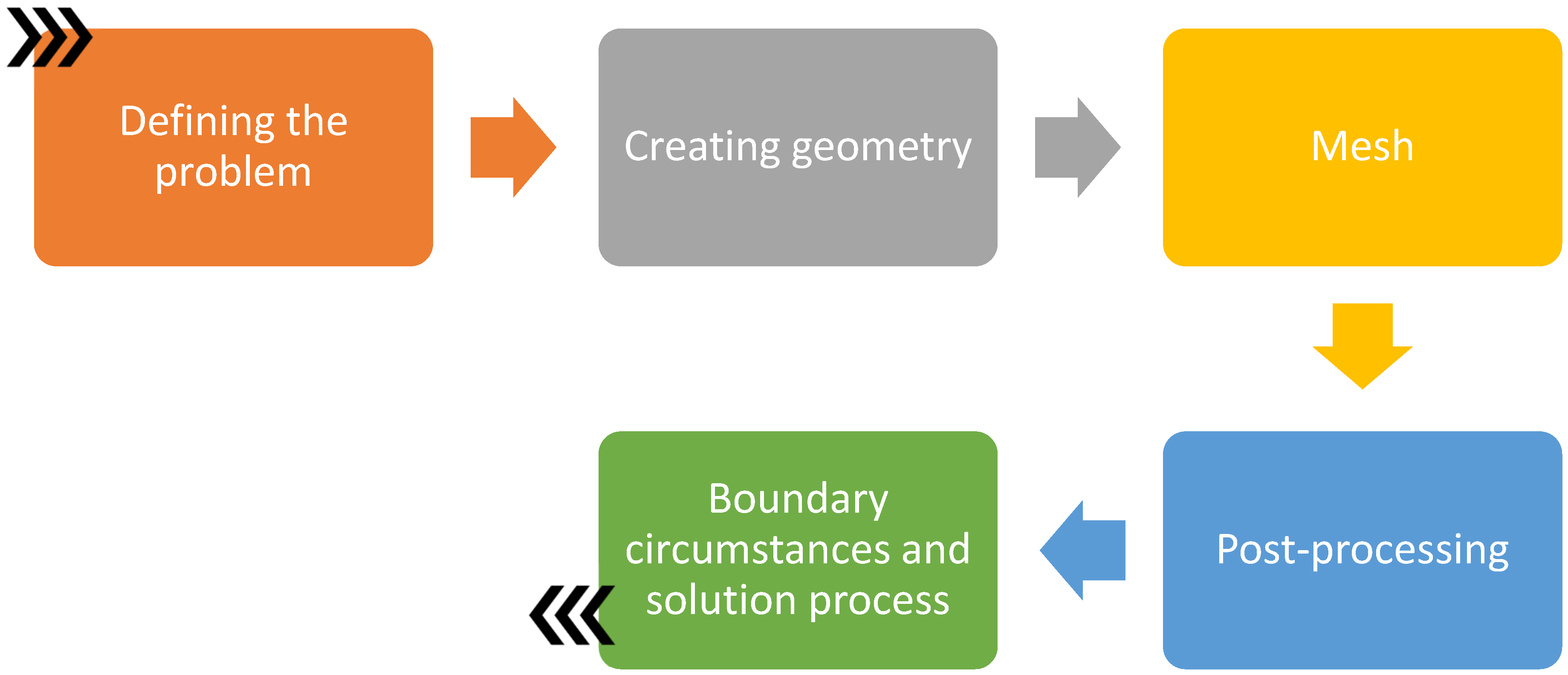
Precise and reliable results were obtained using a CFD solver that complied with NIST standards. The mesh generation process was optimized via meshing sensitivity analysis, and the effects of different mesh sizes on the results were evaluated. A flowchart of the methodology is presented in
Chart 1.
2. Materials and Methods
In the model used in this study, the Reynolds number was greater than 4000. Therefore, the flow was turbulent. For this reason, the k-epsilon turbulent model, which is one of the turbulent models compatible with the model we use when analyzing in Fluent, was used.
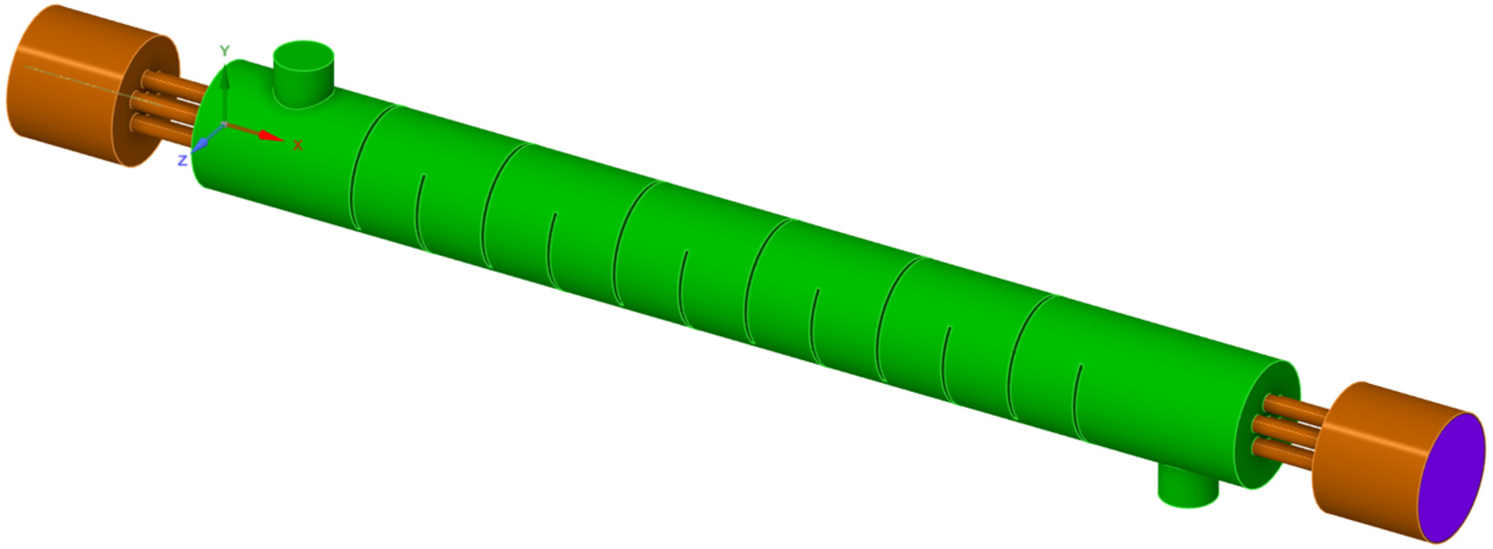
The geometry of the 12-pass tube-type heat exchanger is illustrated in
Figure 1. It was created in 3D in accordance with computational fluid dynamics simulations. This geometry contains three volume geometries: the shell flow volume shown in green, the solid volume containing metal pipes shown in brown, and finally, the tube-pipe flow volume shown in purple.
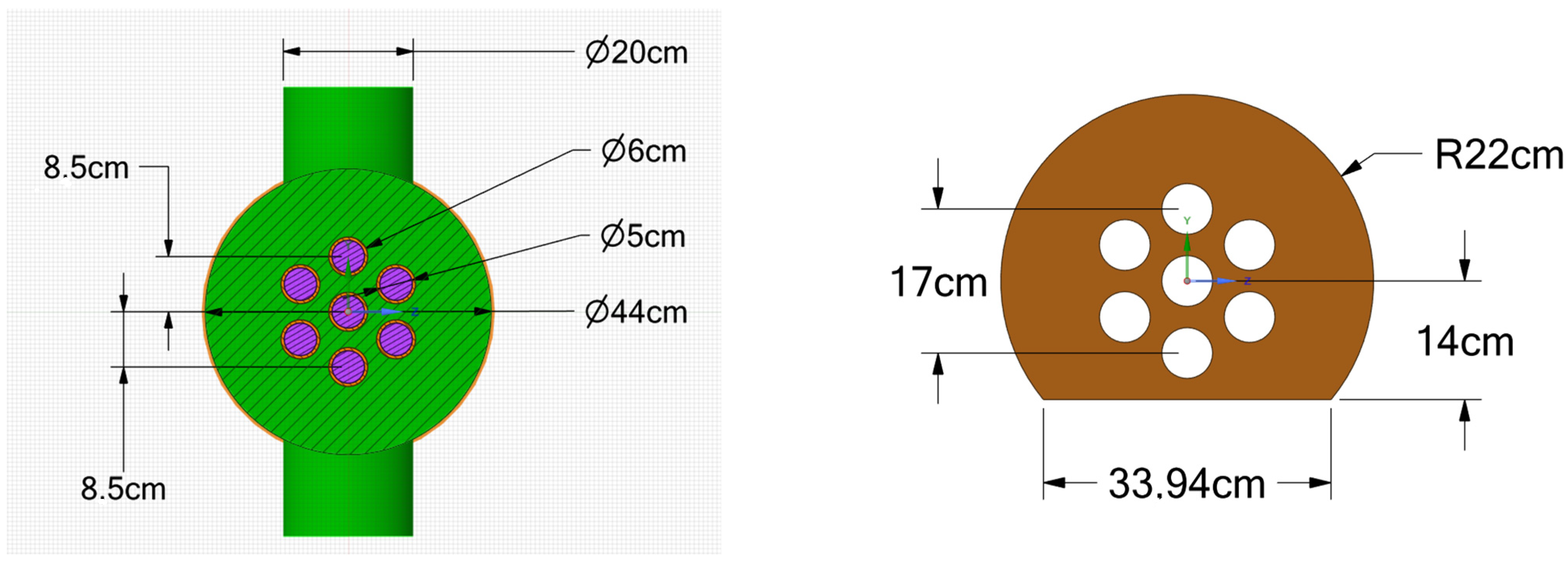
The figure shows a baffle with a thickness of 1.5 cm, through which seven pipes pass. The inner diameter of the pipes was 5 cm, the outer diameter was 6 cm, and the distance between the centers was 8.5 cm. The diameter of the region forming the external flow volume was 44 cm.
The baffle plates designed in the analysis had a diameter of 22 cm and a cutting degree of 33.94 cm. The distance between the outer centers was determined to be 17 cm, and it consisted of 12 passes as shown in
Figure 2. Additionally, the distance between the cut point and baffle plate center was determined to be 14 cm.
2.1. Corporal Model
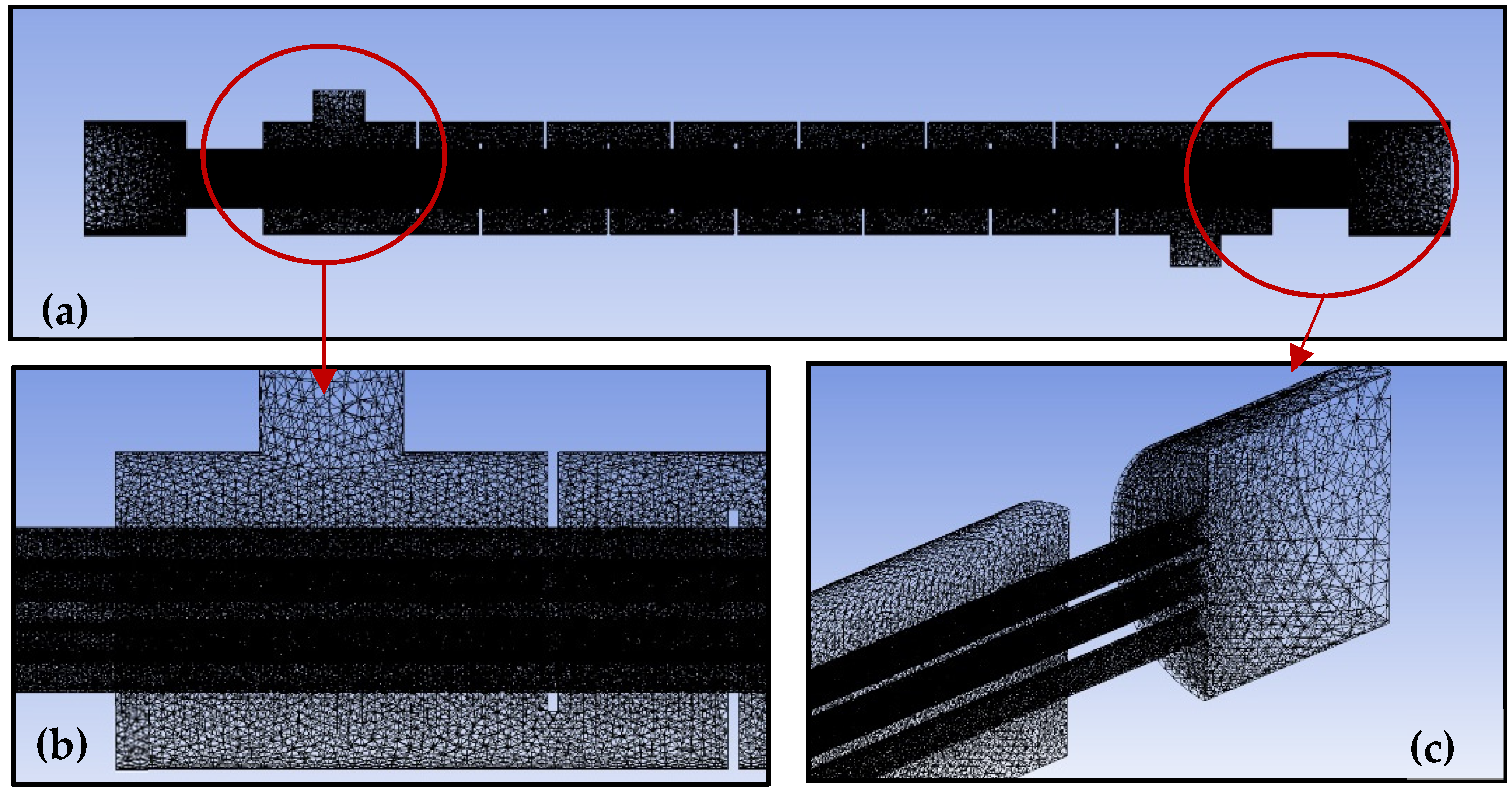
The meshing process in ANSYS Fluent was performed in detail. The structural texture of the model, where the mesh structure was created, was observed in the solution network of the 12-pass tube-type heat exchanger with a total of 3,732,191 elements and 5,839,493 nodes.
In
Figure 3, the mesh structure of the entire model is depicted in image a. The proper mesh structure and quality considerations are highlighted in images b and c, emphasizing the cross-sectional views. In image a shows that whole mesh model. For entry side shows in detail image b. Exit side of the model shows in detail image c.
Figure 4 provides detailed measurements of the entire model. The body length was 396.5 cm, and the length of the caps was 40 cm. The cap diameter was 44 cm and the wall thickness was 0.5 cm.
Table 1 presents comprehensive measurements, including the preferences and parameters used during the meshing process. The solvent preference for meshing is Fluent, with a quadratic element order and a 5 cm element size. The other essential parameters used in the meshing process are listed in
Table 1. These details offer a comprehensive understanding of the meshing process and parameters used.
The structural texture of the model with a mesh structure can be observed in
Figure 3. Here, in the solution network of the 12-pass tube-type heat exchanger, the total number of elements is 3,732,191 and the number of nodes is 5,839,493.
The mesh structure of the entire model is shown in
Figure 3. In images b and c, a proper mesh structure and quality should be considered by considering the cross-sectional views.
The entire model was measured in detail, as shown in
Figure 4. The body length was 396.5 cm, and the length of the caps was 40 cm. When the cap diameter was 44 cm, the wall thickness was taken as 0.5 cm.
The detailed dimensions of the mesh structure are listed in
Table 1. In the solution network of the 12-pass tube-type heat exchanger, the total number of elements is 3,732,191; the number of nodes is 5,839,493. In addition, when the size of the elements in the mesh structure was 5 cm, the skewness ratio was 0.8.
2.2. NIST Model
NIST is an abbreviation for “National Institute of Standards and Technology”. This organization operates as a federal agency in the USA and is an important institution that works on setting standards, measurement, and calibration in the fields of science, technology, and industrial innovation.
NIST also operates in areas such as computational fluid dynamics within the scope of computer-aided engineering. Computational fluid dynamics uses computer-aided methods to analyze the flow in liquids or gasses using the principles of fluid mechanics. This technique examines the changes in pressure, velocity, temperature, and chemical components of fluids through models and simulations.
NIST performs work in the field of CFD, such as developing standards and verifying and determining the verification criteria. This study aims to create a standard basis for improving the accuracy and reliability of CFD simulations. These standards are designed to make fluid dynamics simulations more precise, accurate, and reliable for various industrial applications.
The use of NIST for CFD makes significant contributions to a better understanding of complex fluid dynamics and the development of engineering solutions in real-world applications. These studies help improve the reliability and effectiveness of fluid dynamics simulations used in various industries, such as aerospace, automotive, energy, civil, and environmental engineering.
To determine an appropriate multiphase model for a shell-and-tube heat exchanger, it is crucial to consider the specific characteristics of the flow and the desired level of accuracy. There is a breakdown of the factors to consider.
2.2.1. Flow Regime
- (a)
Laminar Flow: If flow within the tubes is laminar (low Reynolds number), single-phase models may be sufficient. However, if there is potential for a transition to turbulent flow, a transition model may be necessary.
- (b)
Turbulent Flow: For turbulent flow within tubes, turbulence models such as k-epsilon or Reynolds stress models (RSMs) are commonly employed. These models capture the eddy and fluctuation characteristics of turbulent flow, thereby improving the accuracy of the heat transfer predictions.
2.2.2. Dispersed Phase
- (a)
Bubble Flow: If the dispersed phase consists of bubbles, bubbly flow models are suitable. These models account for the interaction between the bubbles and the continuous phase, considering phenomena such as bubble coalescence and breakup.
- (b)
Droplet Flow: For a dispersed phase that consists of droplets, droplet flow models are appropriate. These models capture the behavior of droplets, including their motion, evaporation, and deposition.
2.2.3. Heat Transfer Mechanisms
- (a)
Conduction: If the primary heat transfer mechanism is conduction, single-phase models may be adequate. However, if the phase change or interphase heat transfer is significant, then multiphase models are essential.
- (b)
Phase Change: Multiphase models with appropriate phase change models are crucial for phase change processes such as boiling or condensation. These models account for the latent heat associated with phase transitions and associated interfacial phenomena.
2.2.4. Computational Efficiency
- (a)
Simple Models: If computational efficiency is a primary concern, simpler multiphase models, such as homogeneous flow models, may be considered. However, these models may sacrifice some accuracy for faster computation.
- (b)
Complex Models: More complex multiphase models, such as discrete-phase models (DPMs), offer greater accuracy but incur higher computational costs. These models are suitable for detailed simulations of the dispersed-phase behavior.
In summary, the choice of a multiphase model for a shell-and-tube heat exchanger depends on the specific flow regime, dispersed-phase characteristics, heat transfer mechanisms, and desired level of accuracy.
In summary, Eulerian–Lagrangian models with the k-epsilon model and a complex heat transfer model were used because they provide the most comprehensive approach to simulate turbulent flow and heat transfer in a shell-and-tube heat exchanger under turbulent flow conditions.
2.3. Boundary Circumstances
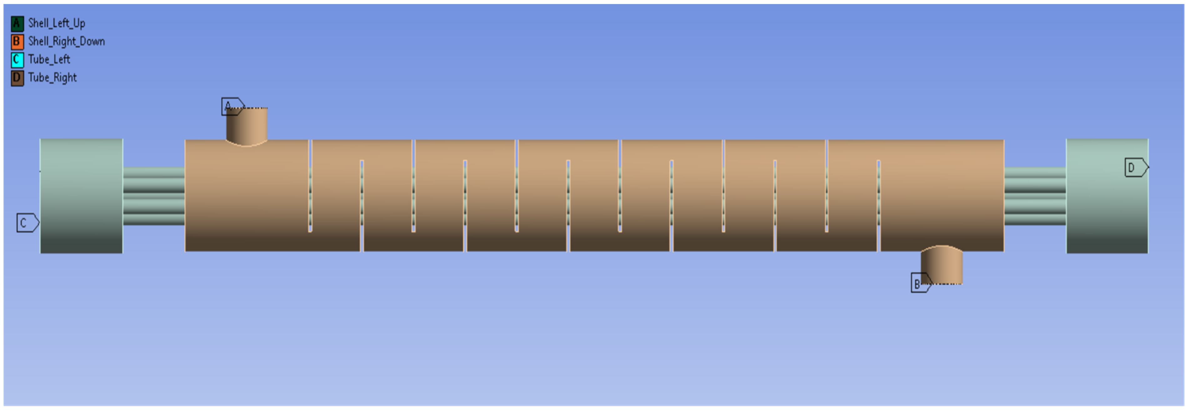
The domain names of the model and the regions where they are defined are indicated in
Figure 5. Accordingly, region A symbolizes the shell’s upper-left region, while region B symbolizes the shell’s lower-right region. Region C is the tube’s left point, and region D is the tube’s right point.
While H2O enters from the shell’s upper-left point, H2O exits from the shell’s lowerright region. While R152a enters from the tube’s left point, R152a fluid exits from the tube’s right point.
3. Results and Discussions
Absolute pressure is less commonly used as a pressure reference because it is always referred to as perfect vacuum or zero pressure. Therefore, absolute pressure is often used as a measurement parameter in specialized applications. Absolute pressure is usually expressed in bars or psi.
The actual pressure at a given location is called the absolute pressure and is measured relative to the absolute vacuum (i.e., absolute zero pressure). The gage pressure is the difference between the absolute pressure and local atmospheric pressure. It can also be expressed as the relative pressure or effective pressure.
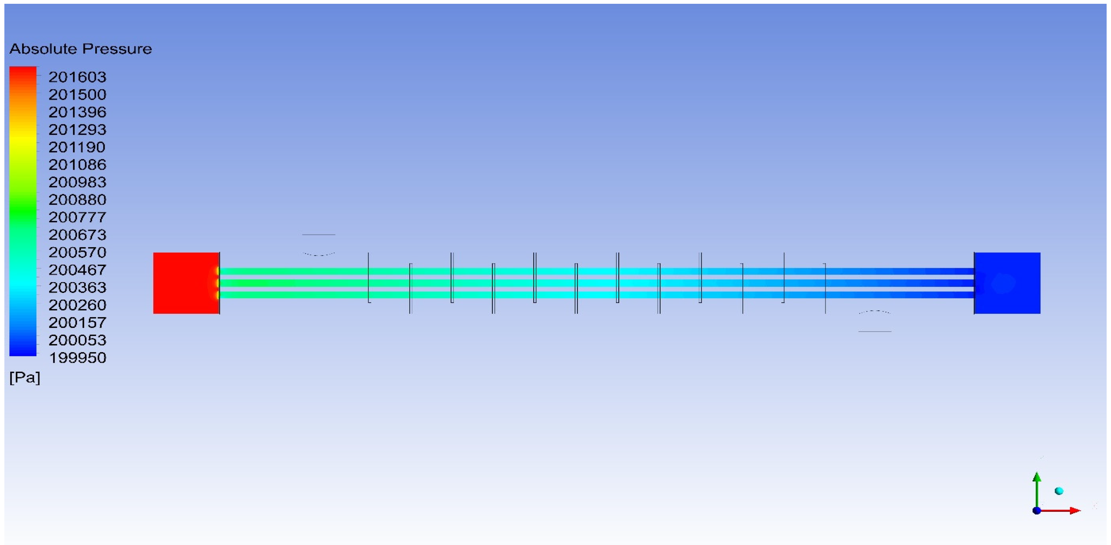
Figure 6 presents a graph representing the absolute pressure values in the internal fluid volume, which shows the pressure changes occurring at the location of the fluid. The curves associated with temperature reveal the change in the absolute pressure of the fluid with temperature. As the fluid moved towards the hot side as it passed through the thin tubes, the absolute pressure increased as the temperature increased. This shows that there is a linear relationship between the temperature and pressure.
Figure 6 shows the absolute pressure of the fluid volume inside the model. The absolute pressure of the fluid inside can vary between 199,953 Pa and 201,603 Pa. As the absolute pressure of the fluid passing through the thin pipes moves towards the hot side, the absolute pressure increases owing to the increase in temperature and can hover in the yellow–green region between 200,362 and 200,786 Pa.
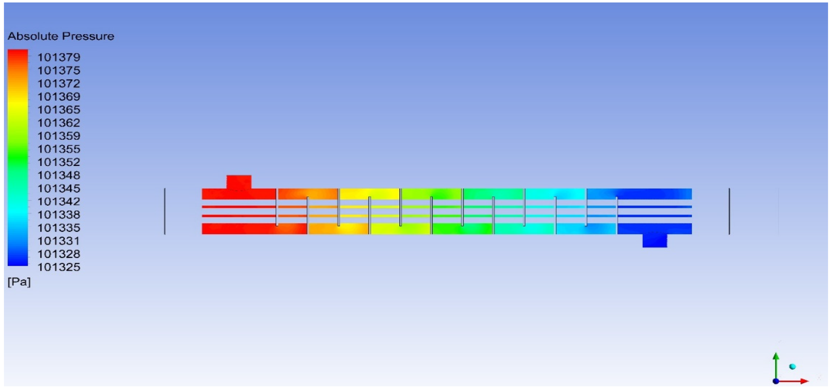
Figure 7 shows the absolute pressure of the fluid volume outside the model.
Figure 7 shows the absolute pressure values for the external fluid volume. Compared with the internal fluid, the pressure changes in the external fluid were lower. The absolute pressure of the external fluid generally varies at lower values than those of the internal fluid. Changes in pressure values outside the volume were more stable and lower than the pressure changes in the internal fluid.
Although the absolute pressure of the inner fluid varies between 199,953 Pa and 201,603 Pa, the absolute pressure of the outer fluid volume can vary between 101,327 Pa and 101,378 Pa. As the absolute pressure of the fluid passing through the body moves towards the hot side, the absolute pressure increases owing to the increase in temperature and can hover in the red–orange region between 101,368 Pa and 101,378 Pa.
In summary, these graphs reveal the thermodynamic properties of the system by showing the changes in the absolute pressures of internal and external fluids. The pressure changes as the temperature increases, and the shape of the pressure differences between the internal and external fluids can be observed in these graphs.
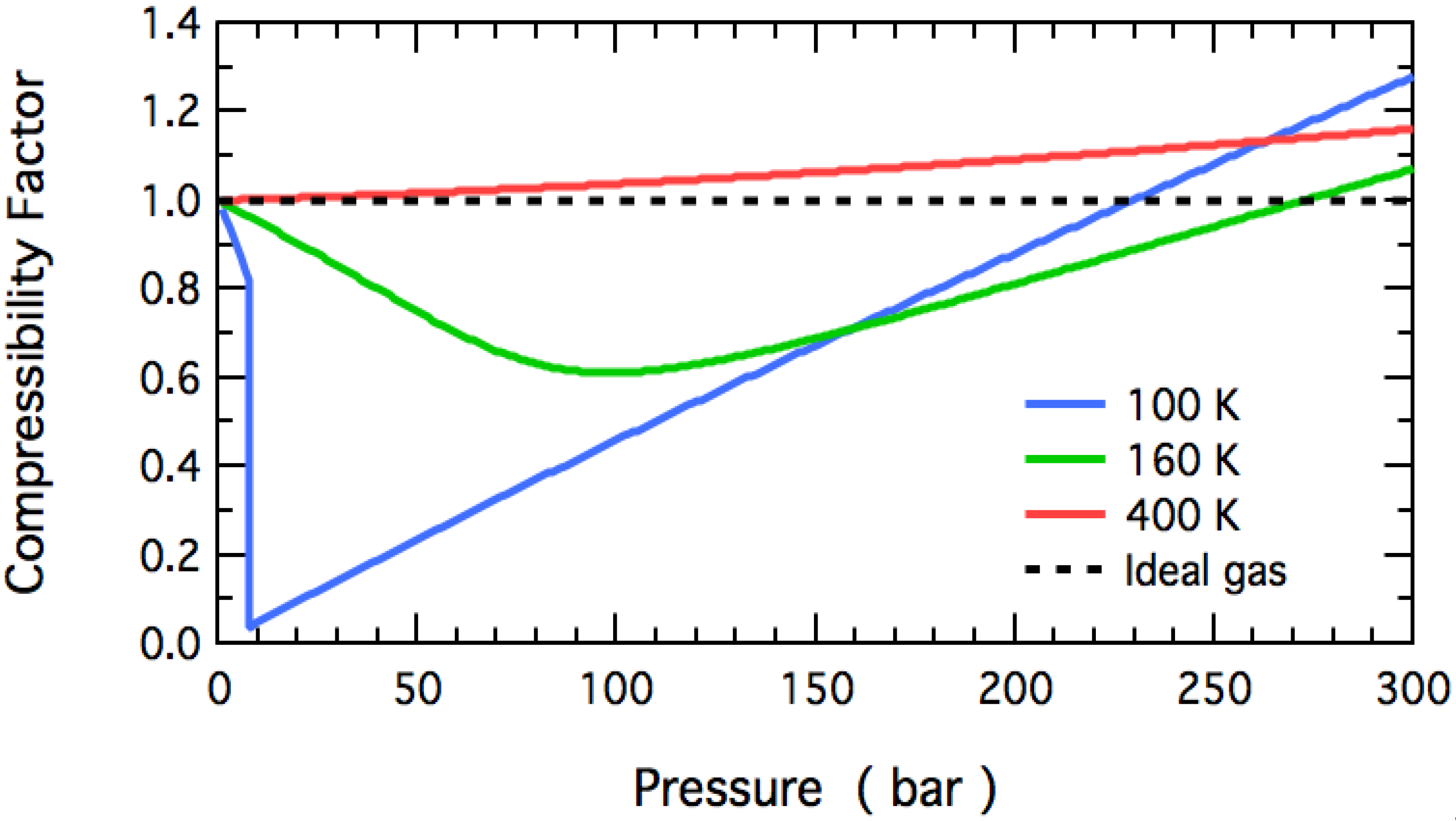
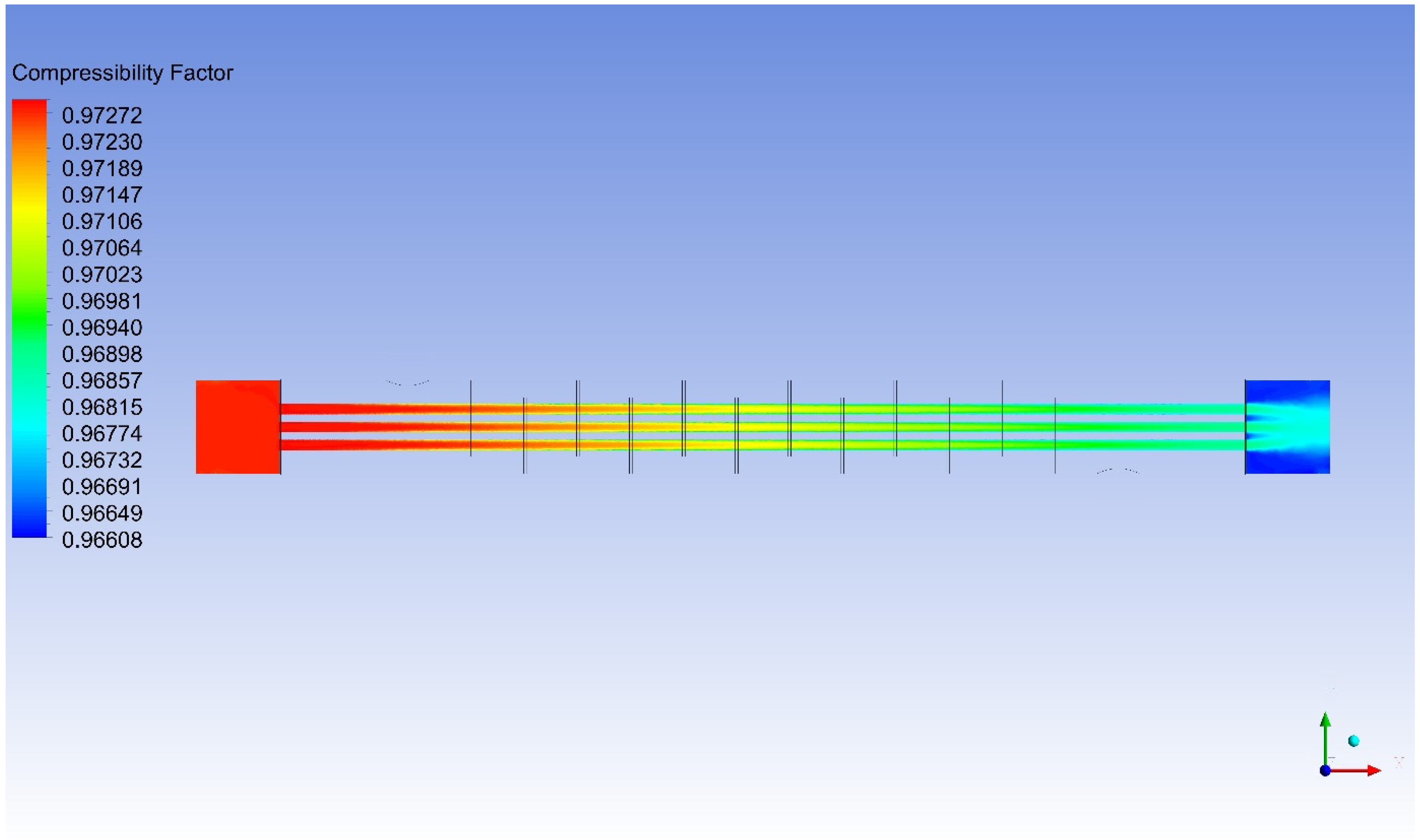
As shown in
Figure 8, for an ideal gas, the compressibility factor will always be unity, equal to one. The compressibility factor, which is usually defined as Z = pV/RT, is unity for an ideal gas. It should not be confused with the isothermal compressibility coefficient. In most engineering work, the compressibility factor is used as a correction factor for ideal behavior.
Figure 9 shows the simulation of the compressibility factor values of the model.
The compressibility factor of R152a of the analyzed model is observed in
Figure 9. If this value is exactly one, it is concluded that it is an ideal gas. The result of the ideal gas behavior of the R152a refrigerant used in the analysis is illustrated. How close R152a is to the ideal gas can be observed as a result of the analysis with the resulting scale. The fact that the values in the graph are close to one indicates that R152a generally behaves like an ideal gas and can provide the desired performance in the system. The scale range is observed between a minimum of 0.96608 and a maximum of 0.97272, and can be observed as being close to ideal gas behavior. At the points where the temperature increases, it comes very close to the ideal gas behavior with a value of 0.97272, and in the colder parts, it moves away from the ideal gas behavior with a minimum value of 0.96608.
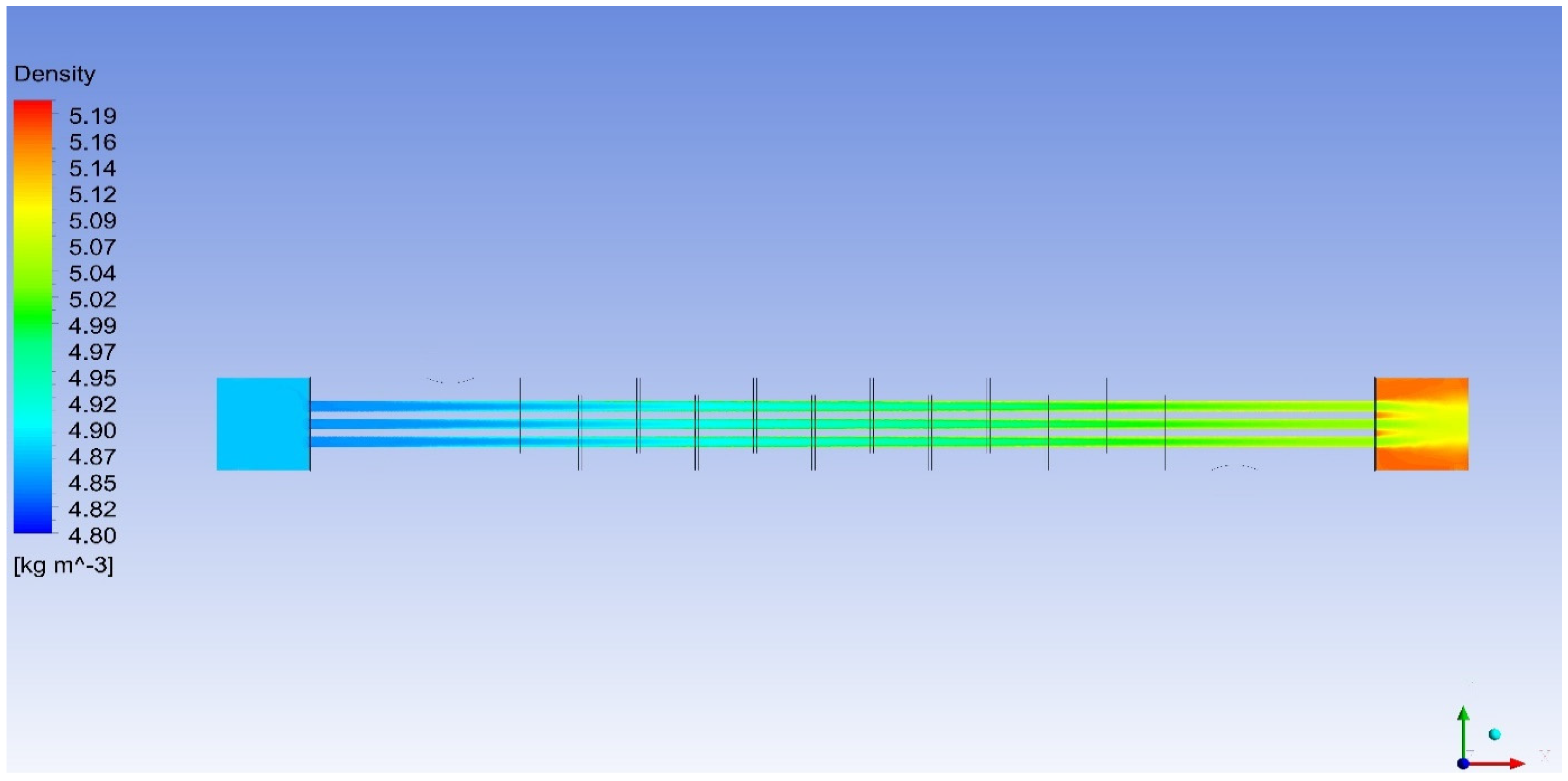
Figure 10 and
Figure 11 are graphs showing the density distribution in the inner and outer fluid volumes. Density changes with temperature and pressure changes. Color tones in the graphs show how the density varies locally and whether the system is homogeneous. In
Figure 10, the distribution of density contours is simulated for the R152a refrigerant. It was observed that the density decreased to around 4.80 kg/m
3 in areas where the temperature increased. It has been determined that in locations where the temperature decreases, the density increases and hovers around a maximum of 5.19 kg/m
3. In the analysis where changing density values were observed, it could be observed that the R152a refrigerant approached a homogeneous structure.
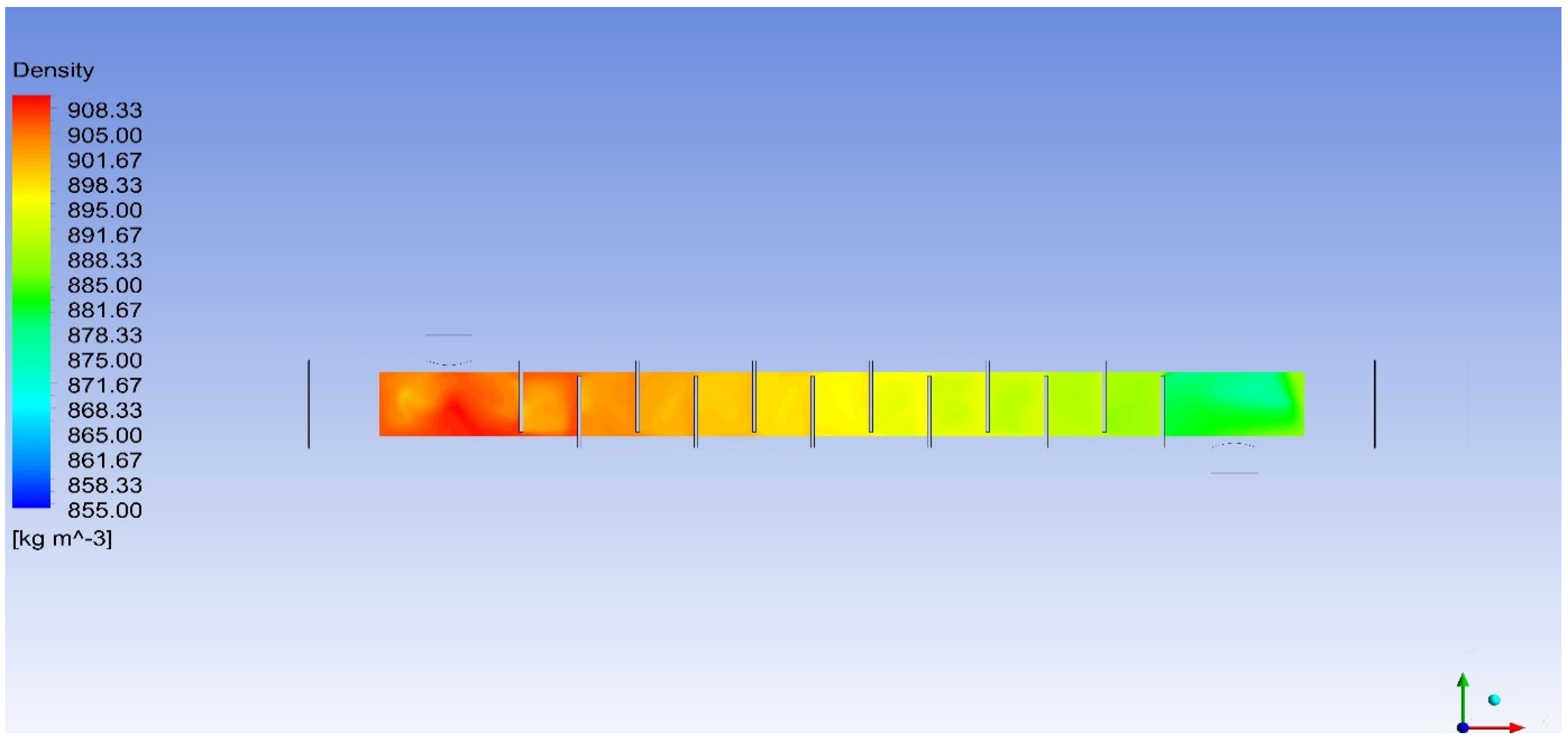
In
Figure 11, the distribution of density contours is simulated for the external fluid volume at Z = p00.0 [cm]. It was observed that the density decreased to around 855.0 kg/m
3 in areas where the temperature increased. It has been determined that in locations where the temperature decreases, the density increases and hovers around a maximum of 908.33 kg/m
3. In the analysis where changing density values were observed, it was observed that the heated water approached a homogeneous structure.
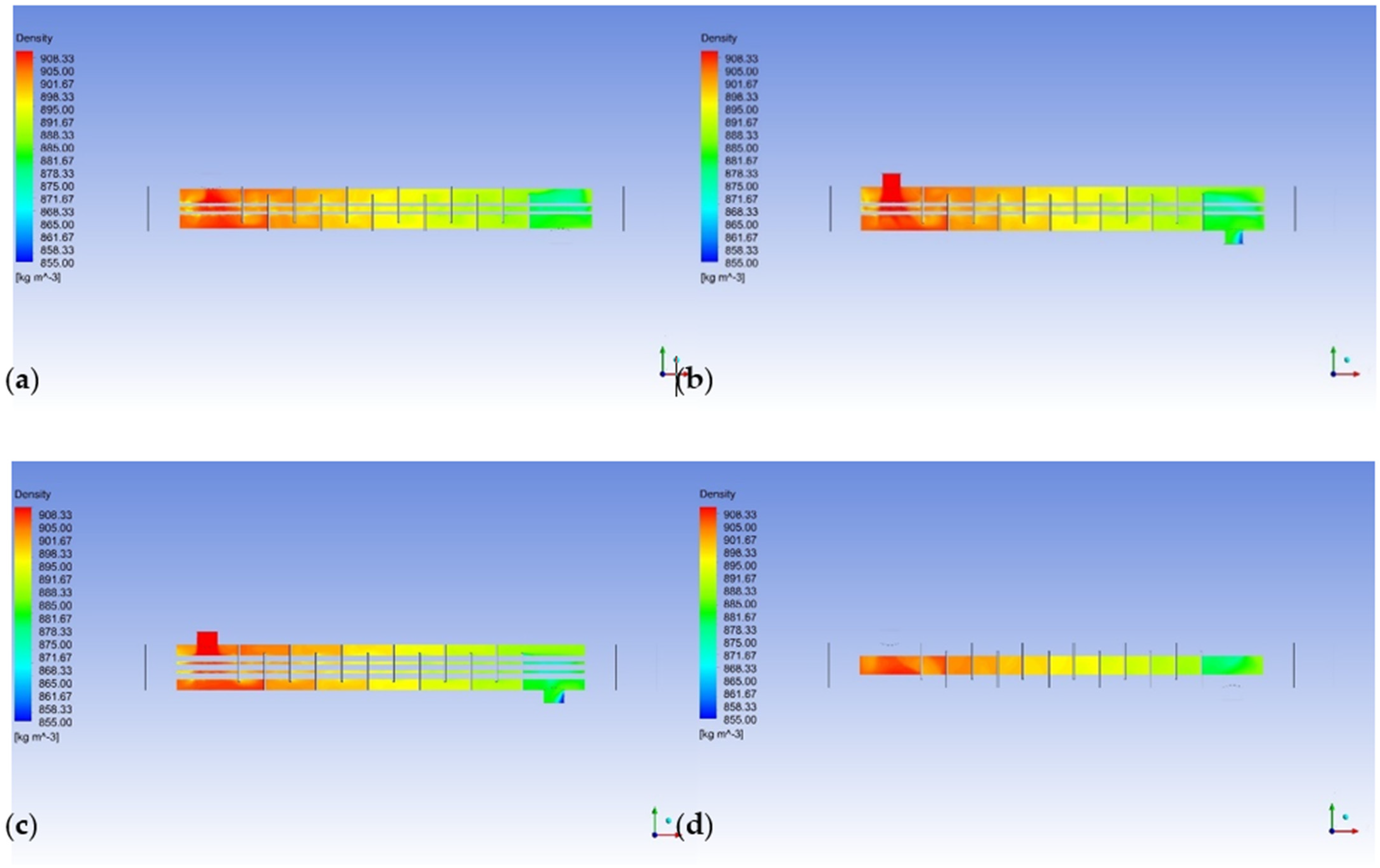
As seen in the distribution of density contours in
Figure 12a–d (Z = p05.0 [cm], Z = p10.0 [cm], Z = p15.0 [cm], and Z = p20.0 [cm]), the external fluid is simulated volume-specifically. It was observed that the density decreased to around 857.01 kg/m
3 in areas where the temperature increased. It has been determined that in locations where the temperature decreases, the density increases and hovers around a maximum of 908.27 kg/m
3. In the analysis where changing density values were observed, it was seen that the observed fluids approached a homogeneous structure.
In fluid dynamics, dynamic pressure (denoted by q or Q and sometimes called velocity pressure) is the quantity defined by
where, in SI units, the following is true:
q is the dynamic pressure in pascals in kg/(m*s2);
ρ is the fluid mass density in kg/m3;
u is the flow speed in m/s.
It can be thought of as the fluid’s kinetic energy per unit volume. In other words, the pressure resulting from the kinetic energy of a fluid is called dynamic pressure [
24].
For incompressible flow, the dynamic pressure of a fluid is the difference between its total pressure and static pressure.
The physical meaning of dynamic pressure is the kinetic energy per unit volume of a fluid. Dynamic pressure is one of the terms of Bernoulli’s equation, which can be derived from the conservation of energy for a fluid in motion [
25,
26,
27,
28].
At a stagnation point, the dynamic pressure is equal to the difference between the stagnation pressure and the static pressure, so the dynamic pressure in a flow field can be measured at a stagnation point.
In
Figure 13, the distribution of dynamic pressure contours is simulated for the R152a internal fluid volume at Z = p00.0 [cm].
Figure 13 and
Figure 14 are graphs showing dynamic pressure values for internal and external fluid volumes. Dynamic pressure represents the kinetic energy of the fluid. The graphs show how the system accelerates and decelerates in different localizations. It was observed that in localizations where the temperature increased, the dynamic pressure value increased to around 1079.26 Pa. In areas where the temperature decreases, it is seen that the dynamic pressure value decreases and hovers around 69.47 Pa. In the analysis where changing dynamic pressure values are observed, it can be observed that the heated refrigerant R152a approaches a homogeneous structure.
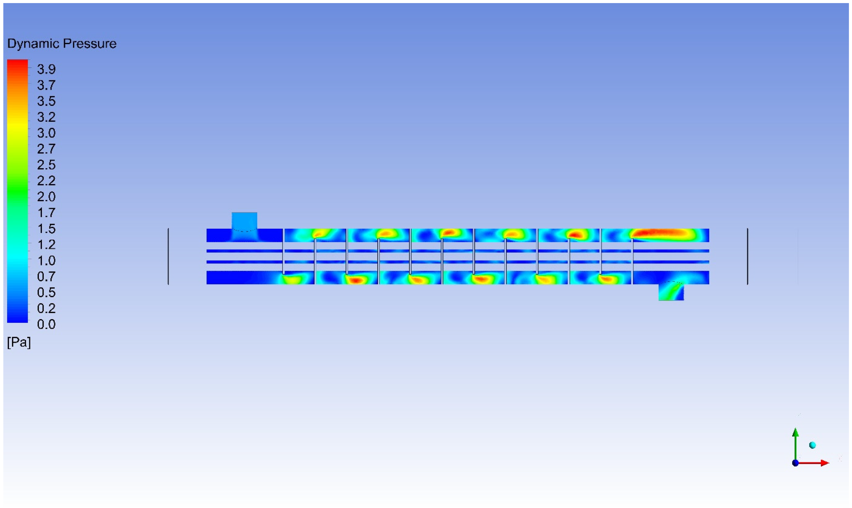
In
Figure 14, the distribution of dynamic pressure contours is simulated for the H
2O external fluid volume at Z = p00.0 [cm]. It was observed that the dynamic pressure value increased to around 3.88 Pa in localizations where the temperature increased. In areas where the temperature decreases, it is seen that the dynamic pressure value decreases and hovers around 0.19 Pa. In the analysis where changing dynamic pressure values are observed, it can be observed that the heated water approaches a symmetrical structure.
Figure 15 and
Figure 16 are graphs showing the distribution of the Prandtl number in the inner and outer fluid volumes. The Prandtl number expresses the ratio of momentum conduction of the fluid to thermal conduction. Values change under the influence of temperature and pressure drops.
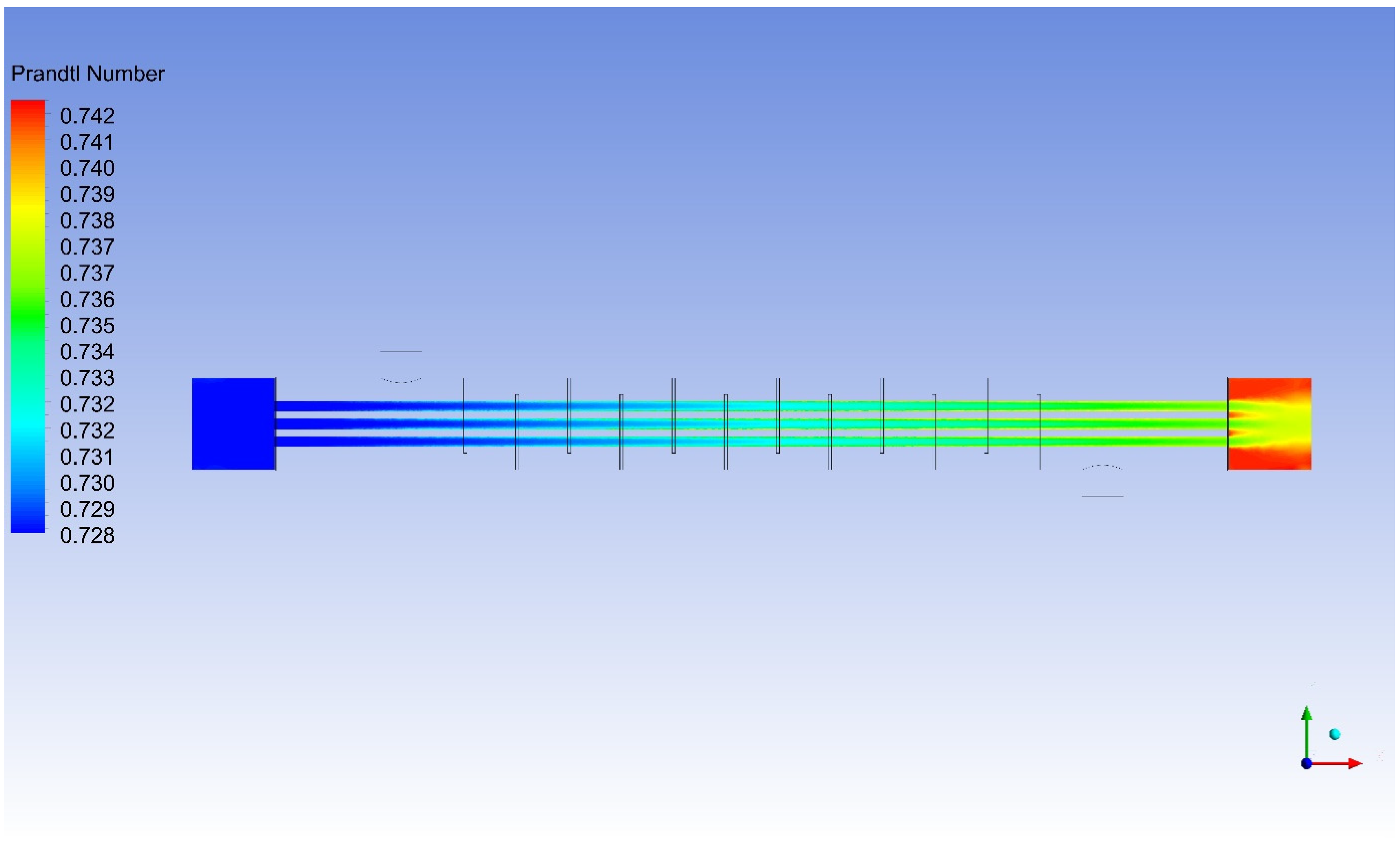
The Prandtl number (Pr) is a dimensionless number. It is the ratio of momentum diffusivity to thermal diffusivity. The number is named after the German physicist Ludwig Prandtl. In
Figure 15, the distribution of Prandtl number contours is simulated for the R152a internal fluid at Z = p00.0 [cm].
This number is defined as follows:
, kinematic viscosity, (m2/s);
a, thermal diffusion coefficient, (m2/s);
, dynamic viscosity, (Pa s = (N s)/m2);
k, thermal conduction coefficient, (W/(m K));
cp, specific heat, (J/(kg K));
, density, (kg/m3).
Unlike the Reynolds number and Grashof number, the Prandtl number depends only on the type and state of the fluid. For this reason, the Prandtl number is frequently included next to property tables where the viscosity and thermal conductivity coefficient of fluids are shown.
The following are some typical values for the Prandtl number (for low Pr, thermal conductivity is strong; for high Pr, thermal convection is strong):
Mercury: 0.015;
Noble gas or hydrogen–noble gas mixtures: 0.16–0.7;
Air and many other gasses: 0.7–0.8;
Between 4 and 5 for R-12 refrigerant;
Seven for water (20 degrees Celsius);
Engine oil: 100–40,000,
Earth’s mantle: 1 × 1025.
For mercury, thermal conduction is more effective than thermal convection; thermal diffusion dominates. For engine oil, thermal convection is much more effective in energy transfer. Here, too, viscous diffusion is dominant.
In heat transfer problems, the Prandtl number controls the relative thicknesses of the viscous and thermal boundary layers. When Pr is small, this indicates that heat is diffusing too quickly. This means that, in liquid metals, the thermal boundary layer is much larger than the momentum boundary layer. Additionally, the equivalent of the Prandtl number in mass transfer is the Schmidt number.
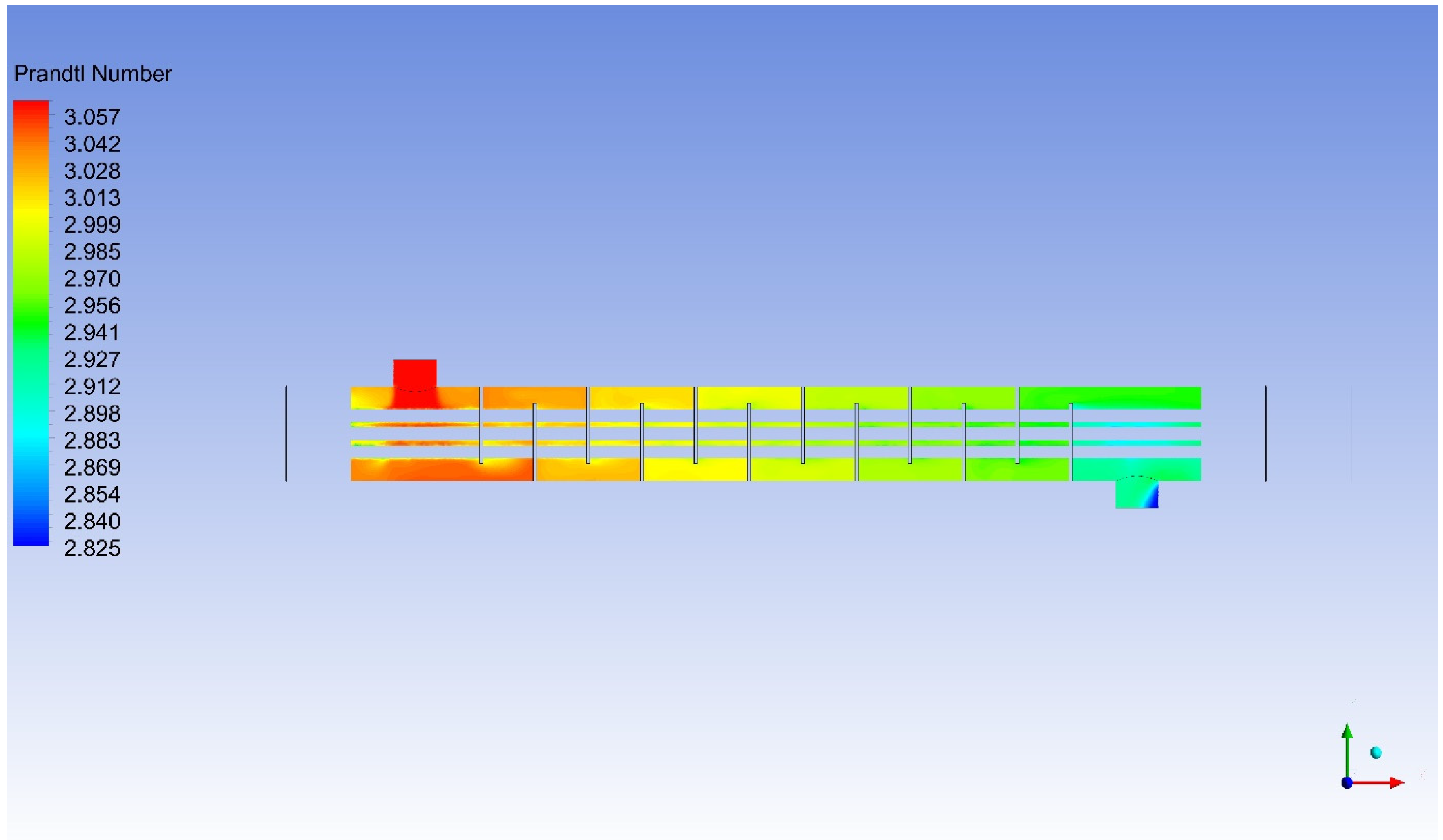
In
Figure 16, the distribution of Prandtl number contours is simulated for the H
2O external fluid volume at Z = p00.0 [cm]. It was observed that the maximum value of the Prandtl number increased to around 3.056 with the effect of temperature and pressure drops. In locations where the temperature decreases, the Prandtl number value decreases and hovers around 2.828. In the analysis where changing Prandtl number values are observed, it can be observed that the heated water moves away from the homogeneous structure and exhibits divergent behavior.
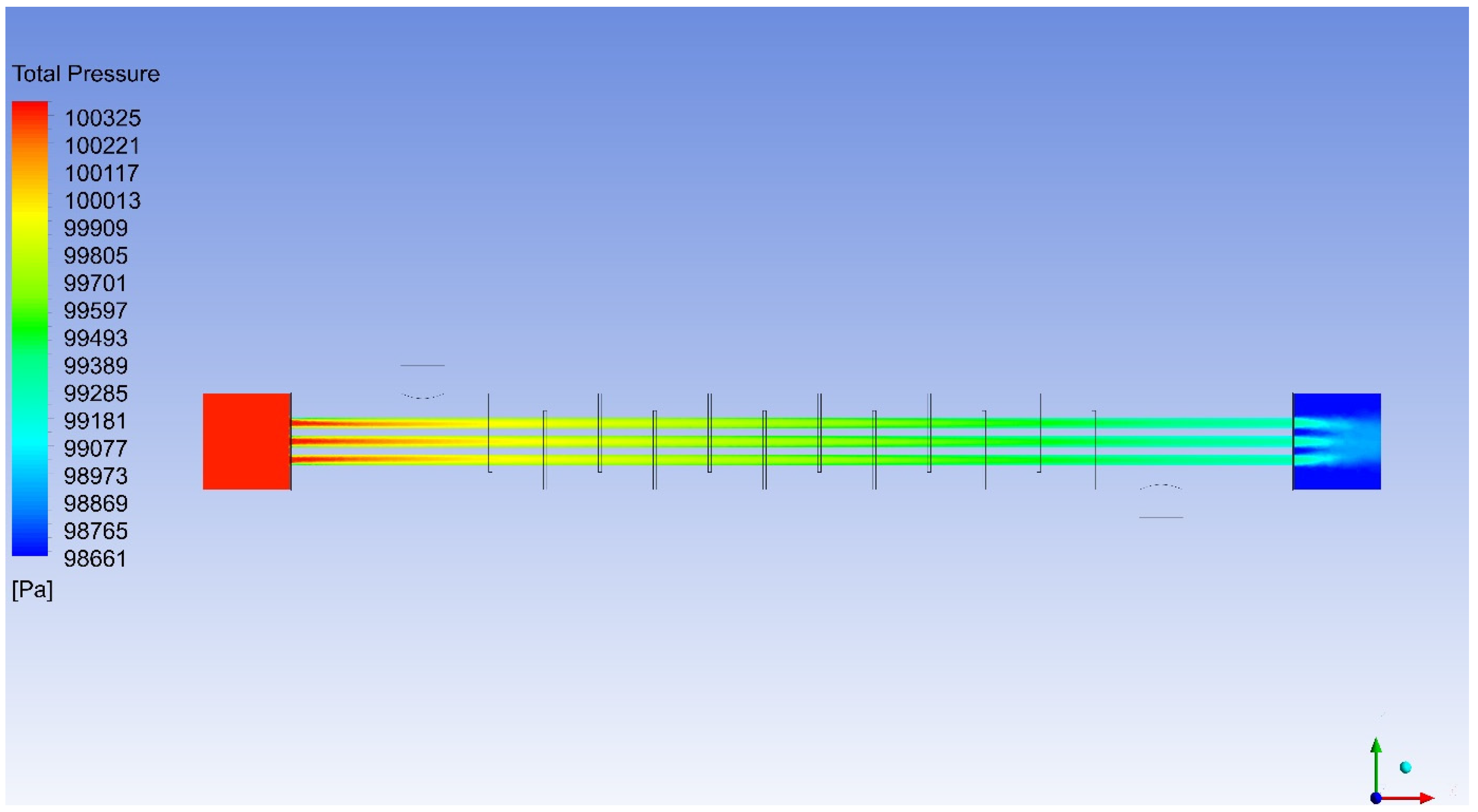
In
Figure 17, the distribution of total pressure contours is simulated for the R152a refrigerant internal fluid volume at Z = p00.0 [cm].
Figure 17 and
Figure 18 are graphs showing the total pressure distribution in the internal and external fluid volumes. Total pressure is an important metric to evaluate the performance of the system. The graphs show the pressure differences at the inlet and outlet areas of the system.
Total pressure is demonstrated in a simulation in which the behavior of two different fluids with the multiphase effect is examined in the process of cooling the hot water coming from the process with the R152a refrigerant. As a result of the analyses, the total pressure value could reach maximum values of 98,661.28 Pa and 100,324.98 Pa. According to
Figure 17, it is seen that the total pressure value increases to the highest values in localizations where the temperature difference is high; it reaches 100286.54 Pa in the entrance region and 98,891.23 Pa can be observed in the exit region.
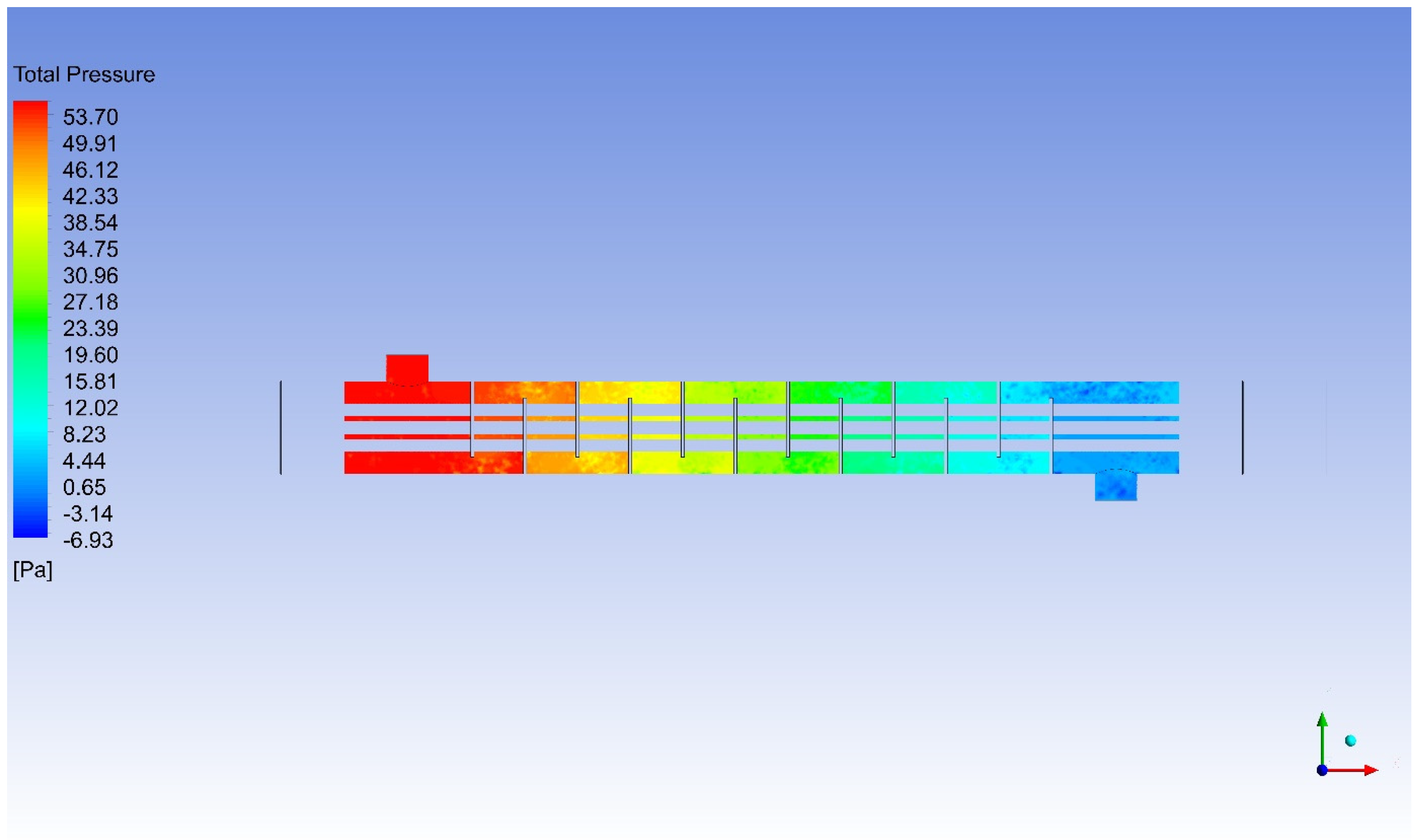
In
Figure 18, the distribution of total pressure contours is simulated for the H
2O external fluid volume at Z = p00.0 [cm]. As a result of the analyses, the total pressure value could reach maximum values of −6.93 Pa and 53.70 Pa. According to
Figure 18, it is seen that the total pressure value increases to the highest values in localizations where the temperature difference is high; it is in the red scale with a value of 52.96 Pa in the entrance region, and can be observed in the blue scale with a value of 6.58 Pa in the exit region.
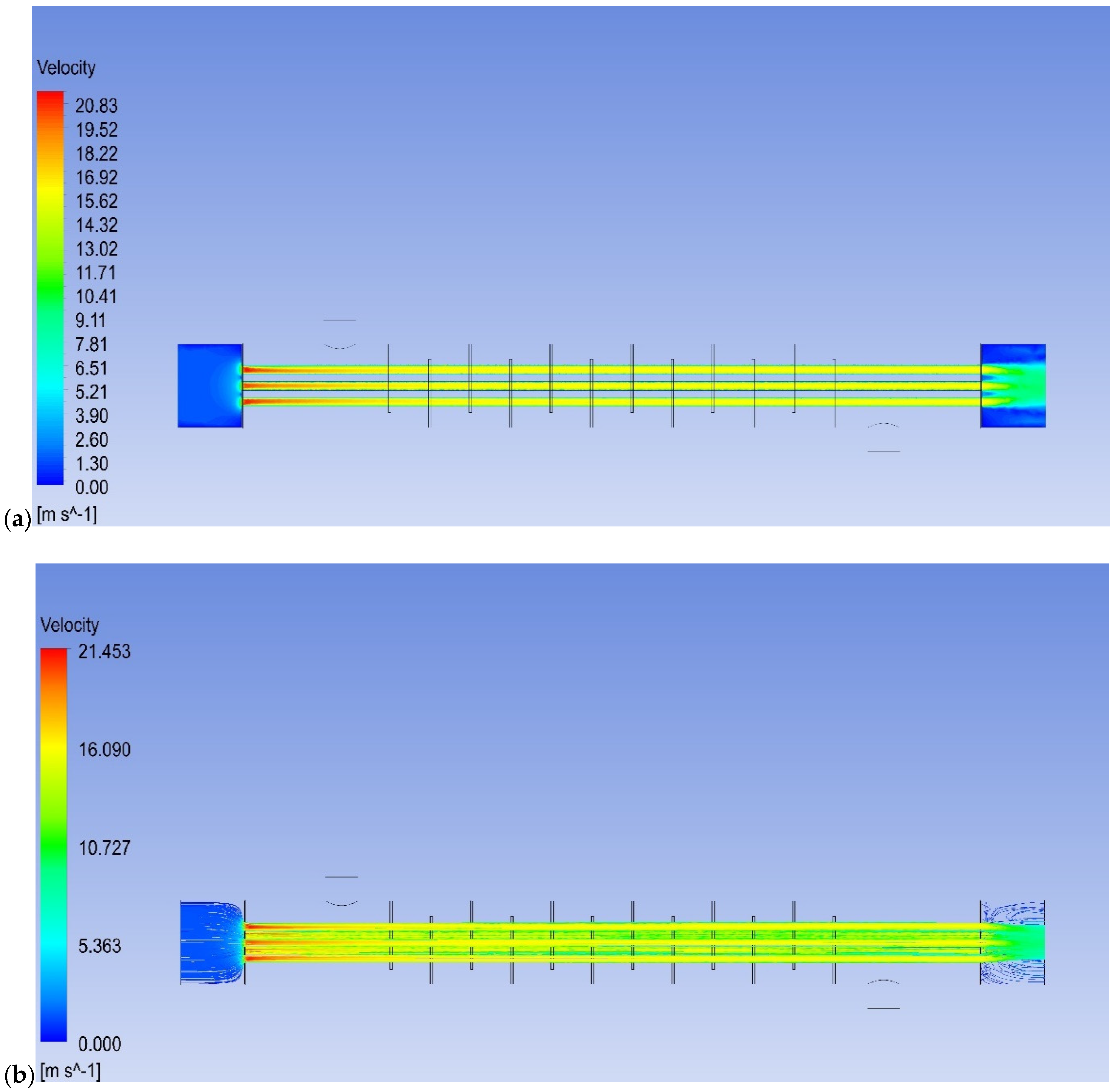
In
Figure 19, the distribution of velocity contours is simulated for the R152a internal refrigerant volume at Z = p00.0 [cm].
Figure 19 and
Figure 20 are graphs showing velocity and flow line contours in the inner and outer fluid volumes. Velocity represents the speed of the fluid, while the flow line shows how the fluid moves along its path. Velocity is demonstrated in a simulation in which the behavior of two different fluids with the multiphase effect is examined in the process of cooling the hot water coming from the process with the R152a refrigerant. As a result of the analyses, the velocity value could reach maximum values of 1.29 Pa and 20.83 Pa. According to
Figure 19, it is seen that the velocity value increases to the highest values in localizations where the temperature difference is high; it is in the red scale with a value of 17.68 Pa in the entrance region, while it can be observed in the green scale with a value of 11.69 Pa in the exit region.
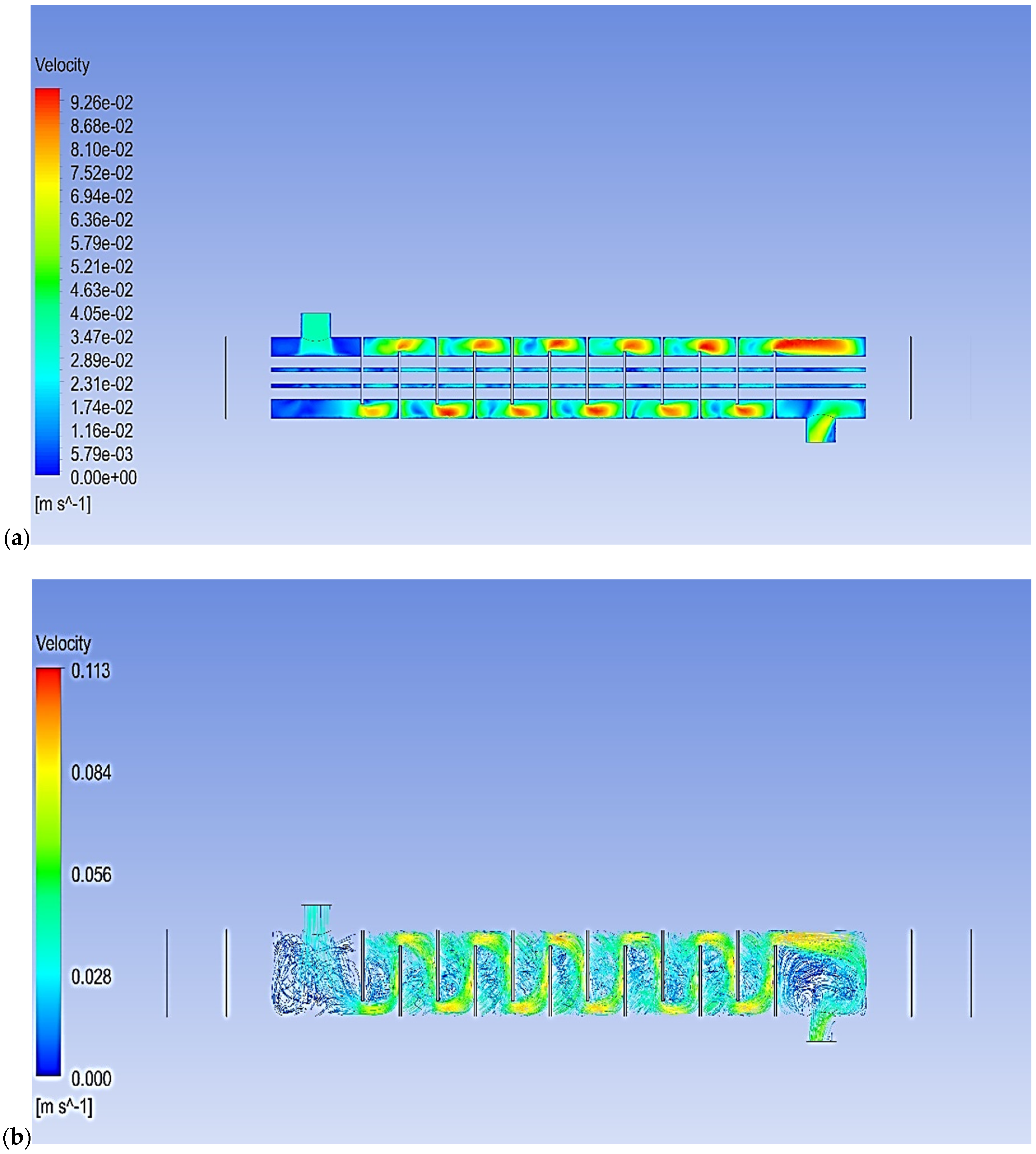
In
Figure 20, the distribution of velocity contours is simulated for the H
2O external fluid volume at Z = p00.0 [cm]. Velocity is demonstrated in a simulation in which the behavior of two different fluids with the multiphase effect is examined in the process of cooling the hot water coming from the process with the R152a refrigerant. As a result of the analyses, the velocity value could reach maximum values of 0.0117 Pa and 0.0926 Pa. According to the analysis results, where there is a non-homogeneous distribution according to
Figure 20, the velocity value is in the turquoise scale with a value of 0.0229 Pa in the entrance region, while it can be detected in the yellow–green scale with a value of 0.0548 Pa in the exit region.
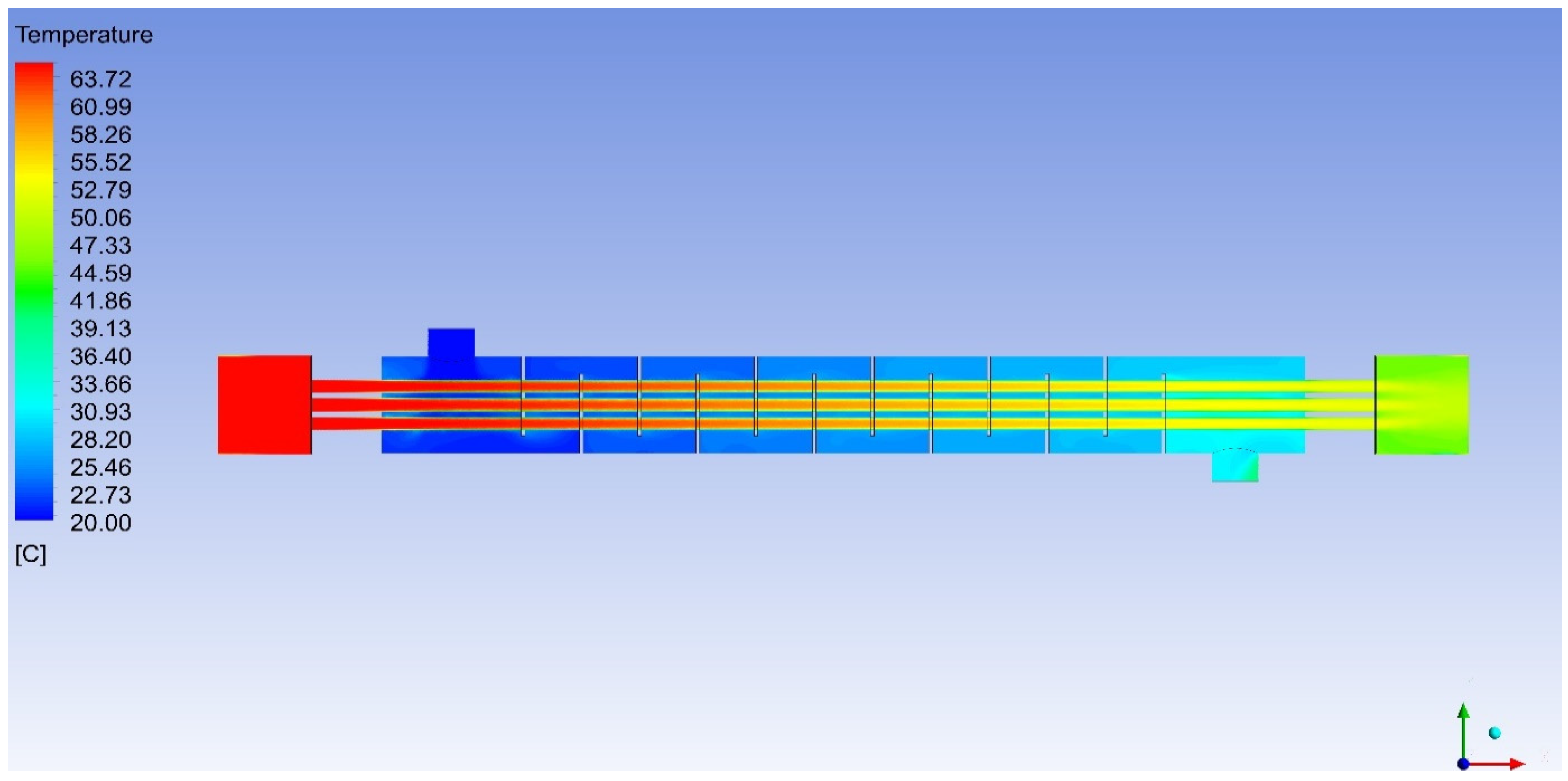
In
Figure 21, the distribution of temperature contours is simulated in a compact manner for H
2O and R152a at Z = p00.0 [cm], specific to the inner and outer fluid volumes.
Figure 21,
Figure 22 and
Figure 23 are graphs showing the temperature distribution in the inner and outer fluid volumes. Temperature changes reflect heat transfer and thermal performance in the system. Temperature differences in the inlet and outlet regions show how heat transfer occurs in the system. Temperature distributions are shown in a simulation in which the behavior of two different fluids with the multiphase effect is examined during the cooling of hot water coming from the process by the R152a refrigerant. As a result of the analysis, the temperature value could reach maximum values of 20.59 °C and 63.58 °C. According to the analysis results, where there is a distribution with transitions according to
Figure 21, the temperature value is in the red scale at 60.98 °C in the entrance region, while it can be detected in the green scale at 42.79 °C in the exit region.
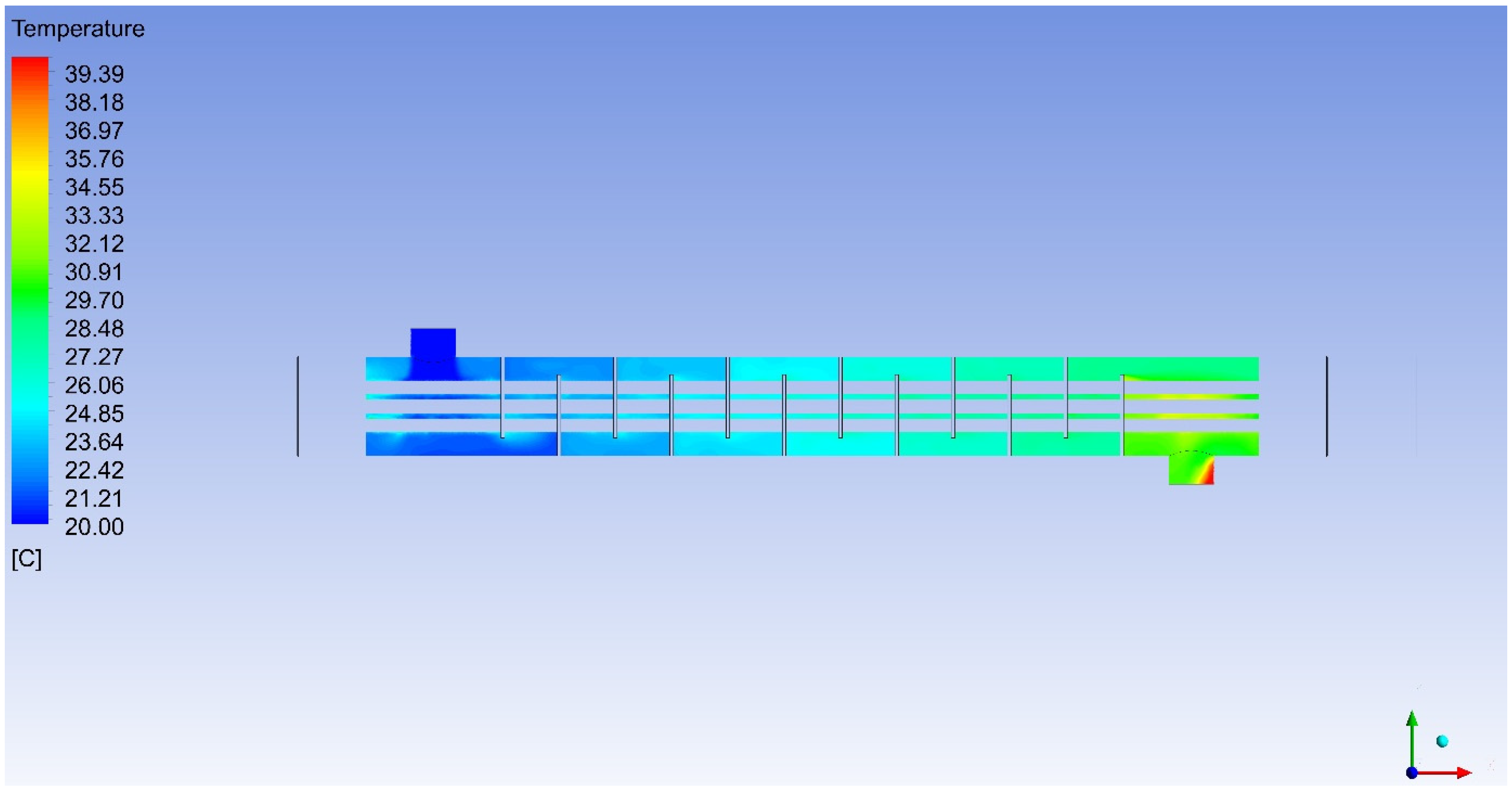
In
Figure 22, the distribution of temperature contours is simulated for H
2O specific to the external fluid volume at Z = p00.0 [cm]. Temperature distributions are shown in a simulation in which the behavior of two different fluids with the multiphase effect is examined in the process of cooling the hot water coming from the process with the R152a refrigerant. As a result of the analysis, the temperature value could reach maximum values of 20.39 °C and 39.39 °C. According to the analysis results, where there is a distribution with transitions in the blue–green scale according to
Figure 22, the temperature value is in the turquoise scale at 23.56 °C in the entrance region, while it can be detected in the green scale at 30.92 °C in the exit region.
In
Figure 23, the distribution of temperature contours is simulated for R152a at Z = p00.0 [cm], specific to the internal fluid volume. Temperature distributions are shown in a simulation in which the behavior of two different fluids with the multiphase effect is examined during the cooling of hot water coming from the process by the R152a refrigerant. As a result of the analysis, the temperature value could reach maximum values of 45.01 °C and 63.98 °C. According to the analysis results, where there is a distribution with transitions in the red–turquoise scale according to
Figure 23, the temperature value is in the red scale at 63.16 °C in the entrance region, while it can be detected in the turquoise scale region at 50.27 °C in the exit region.
This comprehensive computational study analyzed the thermal performance and energy efficiency of using the R152a refrigerant in a parallel-flow heat exchanger. The simulations examined various parameters, including pressure drop, compressibility factor, dynamic pressure, Prandtl number, total pressure, and flow velocities. The results demonstrated that the energy efficiency and thermal performance of R152a are influenced by both fin spacing and flow rates.
Comparison of R152a with Other Refrigerants:
R152a’s performance can be compared with commonly used refrigerants like R134a and R32 based on the following parameters:
Energy Efficiency: R152a can offer higher heat transfer efficiency while consuming less energy compared to R134a and R32 in the heat exchanger. This makes R152a a more environmentally friendly and economical choice.
Thermal Performance: R152a can operate over a wider temperature range and requires lower temperature differences to achieve the desired cooling effect compared to R134a and R32. This makes R152a an ideal candidate for low-temperature refrigeration applications.
Environmental Impact: R152a has a significantly lower GWP than R134a and R32. This means that R152a is more effective in reducing greenhouse gas emissions and protecting the ozone layer.
Further research is recommended on the use of R152a in heat exchangers. This could include nanomaterial applications to enhance the performance of heat exchangers. This could involve studying how nano-coatings and nano-fluids can impact the heat transfer capacity and energy efficiency of R152a.
R152a has emerged as a promising refrigerant offering high thermal performance and energy efficiency in heat exchangers. Its low GWP and environmentally friendly nature make it an attractive option for sustainable refrigeration technologies.


