Abstract
The maintenance strategies commonly employed in industrial settings primarily rely on theoretical models that often overlook the actual operating conditions. To address this limitation, the present paper introduces a novel selective predictive maintenance approach based on a machine learning model for a multi-parallel series system, which involves executing multiple missions with breaks between them. For this purpose, the proposed selective maintenance approach consists of finding, at each breakdown, the optimal structure of maintenance activities that provide the desired reliability level of the system for each mission. This decision is based on a component’s actual age, as determined by the prediction model. In addition, an optimization model with the Extended Great Deluge (EGD) algorithm uses these predictions as input data to identify the best maintenance level for each component considering the constrained maintenance resources. Finally, the numerical results of the proposed idea applied to the Flexible Manufacturing System (FMS) data are presented to show the robustness of the model.
1. Introduction
System reliability and performance are considered one of the central interests in Industry 4.0, given the huge economic losses due to unexpected machine breakdowns. In this case, several maintenance strategies are adopted to avoid these failures and to maintain a system in working order such as preventive, corrective, predictive maintenance activities, and reliability. These strategies aim to ensure a given level of system reliability that allows it to complete the remaining operations with maximum availability [1,2,3]. Moreover, most multi-component systems in industrial applications execute consecutive missions with planned breaks. During these breaks, several maintenance actions can be performed on the various components to improve their lifetime. However, maintaining all components seems very expensive and sometimes unnecessary; thus, selective maintenance aims to determine the optimal number of components and the type of maintenance actions to be performed on the system to successfully achieve the next operation [4]. Such a system may contain manufacturing equipment, aircraft, computer systems, power generation systems, etc. Industrial equipment can operate through the week and be maintained during the weekends or on breaks, the use of the aircraft can be planned, and its maintenance activities between flights and military equipment can be applied to its maintenance actions between missions. In these different cases, maintenance actions should be selected to achieve the desired level of system reliability. At certain maintenance time points, there could be some possibility to plan maintenance actions during the break, e.g., minimal repair, “as bad as old”; different preventive maintenance actions, “a certain level of imperfect maintenance”; or machine overhaul, “as good as new”. After maintenance action, the system should operate with the desired reliability level over the next mission until the next programmed break [5]. Since each of the available maintenance options expends some maintenance means (time, budget, availability of repairman, etc.), it is necessary to allocate resources optimally.
In addition, the selective maintenance strategy has been widely studied in the literature; most existing research has focused on a model where the system degradation follows a stochastic process. However, these proposed maintenance selective strategies are mainly based on theoretical studies and estimated parameters [6]. Furthermore, even if a theoretical or analytical model is created, it is not easy to apply directly in industrial practice with multiple operational variables that exist and can impact the validity of the model over time. To overcome these limitations, artificial intelligence (AI) and machine learning (ML) methods have recently been implemented in several industrial environments to address challenges encountered in model-based approaches. One of the applications of AI is the integration of ML and maintenance, in which companies rely on new types of maintenance for their machines. Such methodology uses predictive tools to estimate when maintenance is necessary. It continuously monitors machine conditions over time and allows for early detection of failures based on historical data. This maintenance strategy is known as predictive maintenance [7]. Therefore, it is possible to collect enormous amounts of real data generated from the various system components, and then learn pertinent information models from these data to use the unhidden designs for decision making in selecting the necessary components that need to be maintained and performing an automatic fault detection to minimize the downtime and related costs and increase the use the components rate [8]. However, in some classical ML models, feature engineering is a necessary technique used to manually manipulate data and create new features to find the best model representing the problem. Since it requires such human experts, artificial neural networks (ANN) show superior performance compared to other machine learning approaches in the automatic extraction of more complex data illustrations and dependencies at high levels of concept, which can also be used in predictive maintenance [9].
This study proposes a new multi-level selective maintenance approach based on a predictive model of a multi-component system by applying supervised ML tools, unsupervised ML methods and metaheuristic optimization methods. Our methodology aims to establish an efficient selective maintenance policy exploiting historical maintenance data. Firstly, a clustering algorithm is used to identify similar components having the same degradation behavior and then to determine the actual age for each component. Therefore, the ANN regression model was exploited to build the actual behavior model capable of predicting the real age of the component system based on the operational and real-world conditions such as number and type of maintenance actions and mean time between failures, etc. The predicted component age is further used in the proposed optimization model to create an optimal maintenance plan. Several intermediate maintenance strategies ( = {1, 2, }) between minimal repair—As Bad As Old (ABAO)—and perfect maintenance—As Good As New (AGAN)—can be applied for each component . Thus, each maintenance policy has an age improvement value, a known maintenance cost and a duration. The resolution method adopted is based on the EDA approach (Extended Deluge Algorithm).
The rest of the paper is structured as follows. In Section 2, we present a literature review on machine learning methods and mathematical models used for predictive maintenance. Problem statements and the optimization model are present in Section 3 which comprises details and notations used in this paper. A description of the proposed approach is provided in Section 4. An illustrative numerical example and results are given in Section 5. In Section 6, we summarize this work in the conclusion and we propose some future axis of research and perspectives.
2. Literature Review
The main bodies of literature related to our study are selective maintenance (SM) and predictive maintenance (PdM). In the literature, the SM problem for multi-component systems was introduced by Rice et al. [10]. The authors studied a serial–parallel system with identical components, the only maintenance strategy available is a replacement and the age of each piece of equipment is exponentially distributed. In addition, to solve the SM problem, the system degradation process is modeled stochastically following an exponential or Weibull distribution which is nearer to reality. Cassady et al. [11] supposed that system component life follows probability Weibull distributions and the decision making is given three maintenance types on failed components: minimal repair, replacement of failed components, and preventive maintenance. Otherwise, in many practical industrial conditions, the system health status and the lifetime distribution parameters of the components after the execution of such missions are uncertain [12,13] and the resources (such as the time allotted to the break and budget) required to achieve maintenance actions are limited. So, the selective maintenance models have been used to increase the system performance and reduce life-cycle cost. Since most of the above works focused on binary systems, Chen et al. [14,15] proposed a new optimization approach to solve the SM problem for a multi-state serial–parallel system. The components as well as the system are considered multi-state, which is more realistic by considering the assumption of binary components. The objective is to minimize the total cost of maintenance by transiting from one state to another for each component and the system. Other SM studies proposed several maintenance options that can be performed to restore the component between AGAN and ABAO is known as imperfect maintenance. These approaches are essentially based on age-reduction models that combine an age-reduction approach with hazard adjustment [16,17]. In this work, the authors developed an age reduction model with an imperfect maintenance action for selective maintenance. They proposed that the age reduction factor depends on the maintenance cost to reflect whether a component is comparatively young or old. So, the component effective age depends on this characteristic constant which helps to establish a relationship between the age reduction factor and component effective age and maintenance cost.
We can notice that all the above-mentioned works propose a model-based approach, with the maintenance model based on theoretical parameters. More recently, with the emergence of new tools such as computer science and the Things Industrial Internet, the maintenance strategies adopted in industrial fields are evolving towards a new PdM policy and condition-based maintenance [7,18,19]. The concept of PdM is to predict the system’s future state early enough based on its actual conditions. Several PdM approaches have been developed in the different production sectors in recent years. Han et al. [20] proposed a new approach for predictive health management of manufacturing systems based on the component’s function. The concept of the predictive strategy involves, as a first step, determining the degradation instrument, functional dependence and remaining useful life (RUL) for the machine system. Then, an operation reliability-focused RUL prediction technique for production systems is established based on the functional dependency of the components. The selected maintenance strategy is based on dynamic RUL prediction, and the functional importance is performed to order the predictive maintenance of component sets. The proposed approach can guarantee the manufacturing system’s ability to complete production operations with high-quality products as well as minimize the maintenance cost in the manufacturing cycle. Thus, the traditional maintenance policy and RUL prediction of manufacturing systems are restricted to the manufacturing components’ performance dependence. In another way, based on the age prediction model that takes into account the dependence of components for product quality necessities, a predictive maintenance approach with the functional importance of components is proposed.
In addition, there are two key models of PdM—data-driven and model-based approaches—and the predicted maintenance structure involves two parts: system age prediction and maintenance plan determination. Several approaches from the research on the topic of selective maintenance strategy for multi-component systems have been studied. A set of operational constraints in selective maintenance optimization is considered, taking into account system and maintenance characteristics and mission profile. Based on these criteria, a general procedure for selective maintenance optimization is developed [4]. The data-based approach shows superior performance compared to the model-based method since the latter requires prior information on the system degradation mechanism; otherwise, the data-based model uses real data to predict the age of the system without knowing the environment of the system degradation process [21].
Generally, a data-driven approach requires several processing methods to extract features from the collected data and to build the best model; such types of requirements involve manual data processing and analysis [22]. Data-driven approaches have the capability to autonomously acquire features that would otherwise demand considerable expertise, time, and experience. Li et al. [23] adopted an advanced fusion technique based on deep random forests to optimize the fault diagnosis performance for gearboxes. This enhancement was achieved by utilizing signals from both acoustic and vibration sensors. He et al. [24] suggested an innovative approach involving a modified deep auto-encoder driven by multi-source parameters. This method was applied to analyze performance degradation parameters from simulation data of aero-engines at the system level and experimental run-to-failure bearing datasets at the component level. Chen et al. [25] introduced an innovative maintenance policy, utilizing a data-driven PdM approach. The decision making for performing maintenance for joint optimization of production and predictive maintenance is determined by introducing a hybrid deep learning technique based on a combination of a long short-term memory (LSTM) and convolutional neural network (CNN) to improve the prediction accuracy of the remaining useful life [26], and by combining the (LSTM) and Markov decision process to provide specific maintenance strategies in different degradation stages of the system [27]. Zonta et al. [28] proposed a model aimed at predictively optimizing maintenance and production schedules using available data. This model generates crucial information empowering decision-makers to minimize production costs.
Different ML techniques have been used by different researchers for building predictive maintenance models from maintenance data. Since the relationship between features is not linear, the techniques used were also nonlinear. The ANN and SVR (Support Vector Machine) are those that have been the most used. However, deep learning approaches have provided an interesting opportunity to develop advanced prediction methods for maintenance data [29]. These models can automatically learn features and extract information despite high levels of abstraction in system data. Recently, artificial neural networks have usually become used in prediction system age and machine failure detection [30,31].
3. Problem Formulation
This section presents a description of the considered problem and the used notations.
Problem Description
The problem studied in this work concerns the multi-series parallel system with independent components (), which is required to perform successive missions alternating with intermission breaks devoted to carrying out selective maintenance actions. The overall aim consists of selecting the best maintenance strategy (also called level) () to perform on component () according to the prediction model, while minimizing the total maintenance cost and maintaining a minimum system reliability. Each component has a set of maintenance strategy ranging from doing nothing () to perfect repair (AGAN with ), in which each is associated with a defined cost. Obviously, the level of component replacement maintenance () is the most expensive of the other levels.
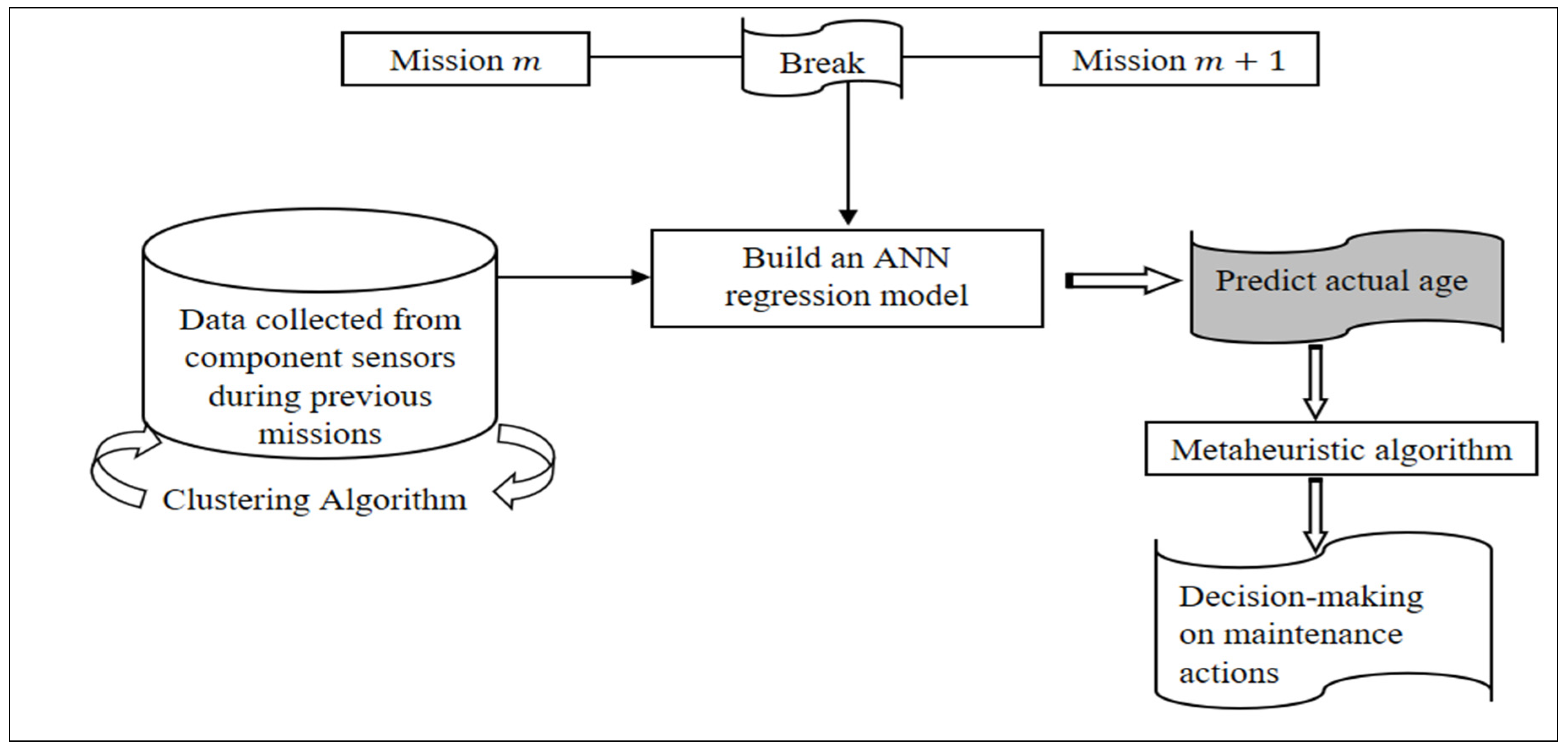
Furthermore, the system state components can degrade due to a number of factors, either functional or environmental, or both, which can lead to a complete system failure and result in its unavailability. As the multi-component system is required to achieve successive missions under a reliability threshold, the actual degradation coefficients of components should be predicted at each break according to the real conditions. These predictions will be used in order to select the best maintenance strategy that ensures a desired reliability level and successfully completes the next mission. Figure 1 illustrates the proposed selective maintenance approach. Actually, the component age provided by the manufacturer does not accurately count the real operational and environmental conditions such as activity frequency, operating time, wear, etc. The real age of a component can be accurately established by predicting its degradation factor according to the real conditions. So, firstly, the proposed approach aims to determine the components real age by computing the age reduction factor using a k-means clustering algorithm, so that the collected data during the operating time can be represented as a matrix form , , where is an -dimensional vector of the component features. Then, the system data collected during previous missions will be used to train the regression model. The model is evaluated with a new dataset in order to be used during the break in building the real system behavior and predicting the actual age components. The ultimate goal is to determine, at each break, the appropriate maintenance strategy for each component based on their actual predicted age. This aims to establish an economical maintenance plan that prevents breakdowns and ensures the system’s reliability.
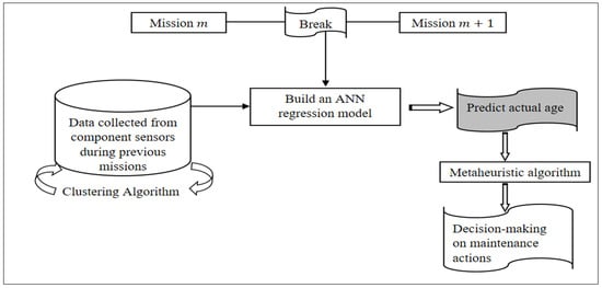
Figure 1.
Overview of the proposed maintenance selective approach.
In addition, the following assumptions are considered to solve the proposed problem:
- Maintenance actions are performed only during the intermission breaks;
- The duration of missions and breaks are assumed known and fixed;
- A minimum threshold of system reliability should be ensured throughout the operating period.
4. Proposed Methodology
4.1. Estimation of Actual Age and System Reliability Function
As the first step, the proposed methodology aims to determine the actual age by calculating the age acceleration factor using the K-means algorithm and then calculating the reliability of the manufacturing system based on a new model that is closely related to the determined actual age [32,33].
The algorithm of k-means clustering allows us to regroup system maintenance data into clusters according to certain features such as number of preventive and corrective maintenance, mean time between failures, etc. Each cluster is represented by a centroid denoted by and a set of components {}. Indeed, to extract similarity between different components, each element is associated with a distance between it and the centroid of the group to which it belongs. Thus, the farthest element from the centroid of the class it belongs to is the “bad-representative-component”, while the “best-representative-component” is the average of all clusters calculated by the mean of all centroids.
So, the component degradation degree can be considered as its deviation from the “most representative component”. Consider is the distance from the “best-representative-component” to the element and is the distance between the best and the bad component. The degradation coefficient is calculated by using Equation (1).
Note that when the component does not deteriorate, and its actual age is as provided by the manufacturer. Otherwise, if is very close to , indicating a maximum degradation, maintenance of the component is necessary to prevent a system breakdown.
Then, the actual age of the components at the end of mission is calculated by Equation (2).
where the theoretical age at the end of mission can be formulated by Equation (3).
To account for the genuine impact of component age on its failure rate, we present a novel formula crafted by amalgamating insights from Ben-salem et al. [34] and Bouslah et al. [35]. The primary goal is to scrutinize system availability, which diminishes with degradation. To achieve this, the authors model the system’s failure rate as a function that grows with the component’s age. In our proposed formula, represented by Equation (4), we define the failure rate of a specific component as a function of its current age, denoted as ).
where , and are system settings depending on the equipment characteristics and its age degradation. Indeed, for such components that have been maintained recently, the failure rate is close to . Otherwise, when the actual age decreases, the failure rate becomes higher until it reaches the sum . In addition, the positive parameter is introduced due to significant variations of the maintenance data and the real conditions that may occur during the period of operation such that the system age degrades when the is important however the system has a low failure rate when the is less significant.
Therefore, the system reliability function is considered closely related to the failure rate and takes into account the degradation of the system lifetime, so that it can be expressed as follows:
4.2. Predictive Model for Multi-Level Selective Maintenance Using ANN and SVR
4.2.1. The General Concept of the ANN Model
The Artificial Neural Network (ANN) is inspired by the architecture of neurons in the brain. To simplify the mathematical modeling, an ANN is composed of a single hidden layer, an input layer and an output layer. Nodes in one layer are linked to nodes in the next layer through weights. Initially, the weights and biases are randomly generated [36,37]. The ANN model is based on the following equations:
where:
- -
- : the input node
- -
- : the output of the hidden node
- -
- : the weight connecting the input node to the hidden node
- -
- : the activation function of the model
- -
- : the input layer bias
- -
- : the hidden layer bias
- -
- : the model output: the estimated target value.
In a neural network, an activation function () is used to choose how the weighted sum of the input is transformed into an output from nodes in another layer of the network. The selection of activation function has a big impact on the neural network performance, and several activation functions may be used in different parts of the model [38,39].
In general, four common functions used in hidden layers are considered as the activation function for the ANN algorithm:
- Identity function
- Logistic Sigmoid function
- Rectified linear unit function
- Hyperbolic tangent function
4.2.2. The General Concept of SVR Model
The Support Vector Regression (SVR) model is a Kernel-based nonlinear learning technique used for regression as well as classification. It consists of defining or creating hyperplanes to discriminate predictions from training data. SVR approximates predictions using a function that has a fixed deviation threshold from the actual targets [40], which is formulated by Equation (13).
where is the transfer function, is an input data point and the parameters and are estimated by solving the following optimization problem stated by Cortes and Vapnik [41].
where is the regulation, is the target, is the size of the training data, is the deviation threshold of the function , is the penalty parameter and is the relaxed error that guarantees the existence of a solution under these constraints.
Note that Equation (13) is useful for solving linear problems, but for nonlinear problems a transformation to a high-dimensional space is necessary. For this, a Kernel function is used which maps the original input data to a higher nonlinear feature space. The Lagrangian form equivalent is given by
where is the Kernel function and , are the Lagrangian multiplier. Four usual Kernel functions are generally used which are linear function, polynomial function, Radial Basis Function (RBF) and Hyperbolic Tangent Function (HTF). In this paper, we will use SVR with linear Kernel function and SVR with RBF Kernel in which their explicit functions are defined by Equation (15) and Equation (16), respectively.
where and are adjustable parameters.
4.2.3. Hyperparameter and Model Evaluation
The model training process involves selecting the optimal hyperparameters that the learning algorithm will use to learn the optimal parameters and properly map the input features (independent variables) to the labels (dependent variables). Hyperparameters are used to control the process of learning and determine the model parameter values that a learning algorithm ends up learning. There are several training techniques introduced into machine learning to find these optimal hyperparameters, and the most widely used method is random search. Indeed, this technique uses a random combination of parameters at each iteration to find the best solution for the built model. In addition, it has been shown theoretically and empirically that a randomized search is computationally efficient, especially when it comes to ANN models [42]. In fact, hyperparameter values should be settled before the training of the model begins. Then, a backpropagation algorithm (BP) is applied to the model in order to find the optimal values of the weights .
In this study, the hyperparameters considered for the ANN model are the number of hidden layers, the number of nodes for each layer and the learning rate of the optimization algorithm used to fit the model. So, defining the network configuration is the first step in developing the model.
Therefore, the second step is to compile and fit the network to build our model. To train the model, the compilation applied an optimization algorithm and a loss function to evaluate the network. As we studied a regression problem, an adaptive optimizer called Adam updates the network weights iteratively, and a mean squared error loss function is implemented to calculate the average differences between the actual and predicted labels [43].
Therefore, in order to evaluate the predictive performances and the accuracy of the model based on ANN or SVR, certain evaluation indices have been used. These indices are explained below and are among the most commonly used performance measures with as the actual value and as the predicted value.
Absolute error (): the absolute error is given by the absolute value of the difference between the measured (actual) value and the predictive value
Mean Absolute Error (MAE): measures the average of absolute errors of predictions and observations
Mean Squared Error (MSE): measures the average squared difference between the observed and predicted values
Mean Absolute Percentage Error (MAPE): a statistical measure to define the accuracy of a machine learning algorithm on a particular dataset. It can be considered as a loss function to define the error termed by the model evaluation
4.2.4. Predictive Model on the FMS Data
Recall that the objective of the proposed predictive model is to estimate at each break the degradation factor of a multi-component manufacturing system on maintenance history based on ANN and SVR regression models. In this sub-section, the model built in our experiments is first presented. Then, we will dive into the optimal hyperparameters of the ANN model. Next, a comparative study is presented between ANN and SVR models based on the performance indices.
The dataset used in this experimental study is obtained from a Flexible Maintenance System (FMS), which contains, after processing, the history of maintenance interventions that are shown in Table 1. Each station of this FMS is composed of more than 264 electrical and mechanical components where for each component the intervention date is recorded, as well as the type of maintenance action either corrective (CM) or preventive (PM), and the failure type that is defined by a code.

Table 1.
Example of FMS data.
Therefore, as explained in Section 4.1, after data processing a second operation is necessary which consists of computing the Mean Time Between Failure (MTBF), Number of Preventive Maintenance (Nb.PM) and Number of Corrective Maintenance (Nb.CM). These values are used to determine the component coefficient degradation by using the k-means clustering algorithm. As the main objective is to build a model able to predict the component coefficient degradation from their real condition after performing some operations, these obtained results are fed into the ANN model for forecasting. For this purpose, this dataset is split into training and evaluation subsets.
The model has been developed in Python with the use of the Keras machine learning library on top of the open-source machine learning framework called TensorFlow. The data has been partitioned by an splitting rule, i.e., of data is used for the training step while is employed to evaluate the model. Then, the info has been scaled to the interval of , which is understood to assist the neural network in learning underlying patterns, both more accurately and more efficiently.
To reach the optimal model hyperparameters, we use the random search method implemented in the Keras tuner library. So, the best configuration of the model found using the random search method is as follows:
- -
- An input layer of nodes and an activation function Relu (rectified linear unit);
- -
- A first hidden layer of nodes and an activation function Relu;
- -
- A second hidden layer of nodes and an activation function Relu;
- -
- An output layer of one node (regression problem).
In addition, the optimal hyperparameters obtained for the SVR model with linear Kernel and with RBF Kernel are , and .
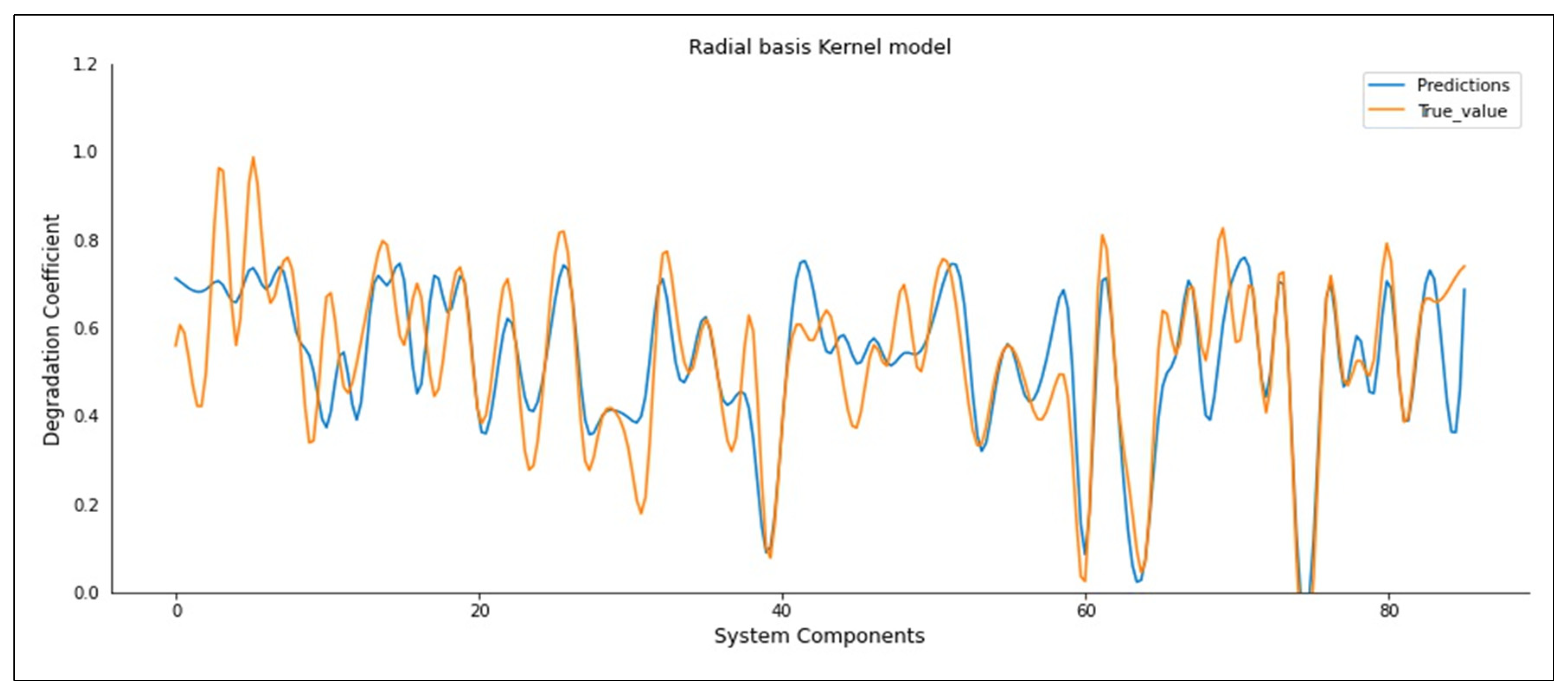
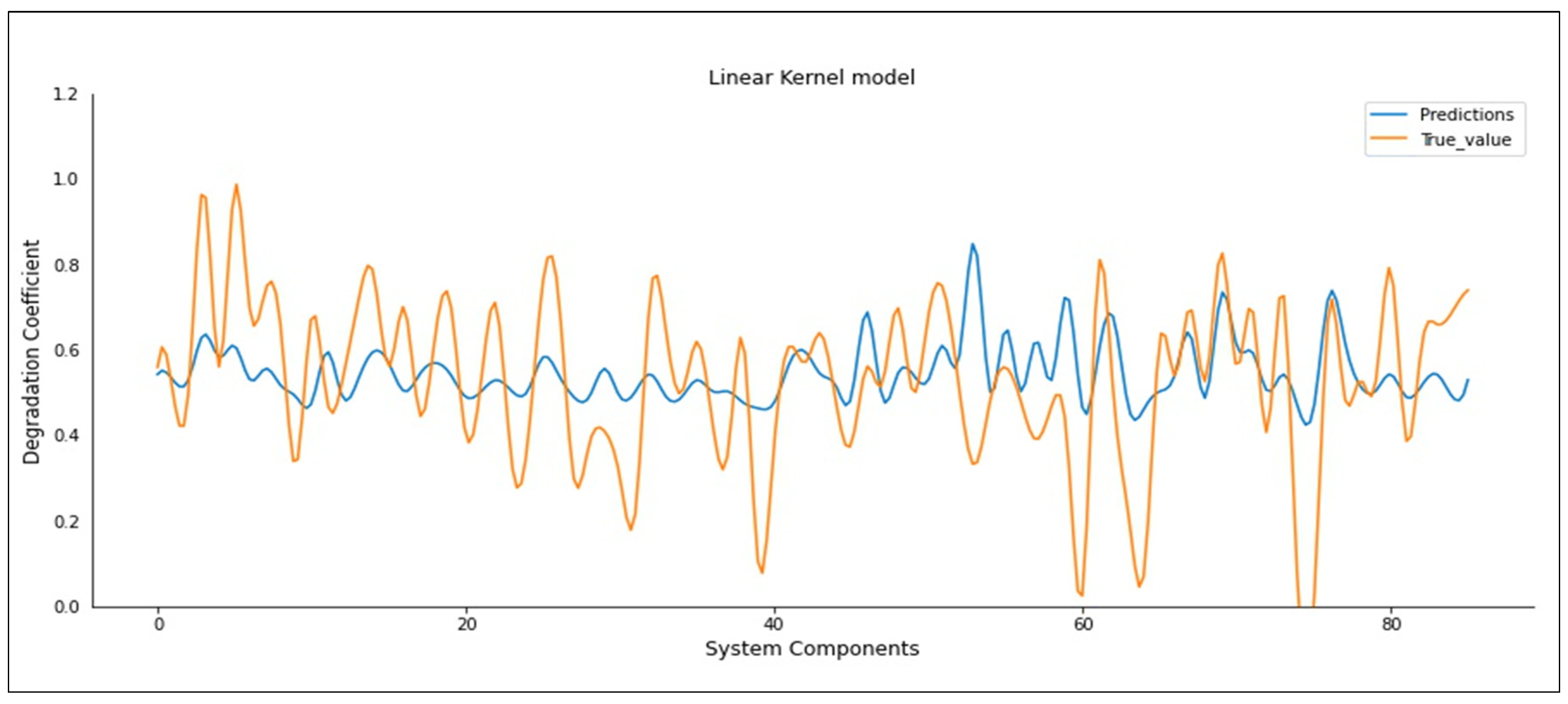
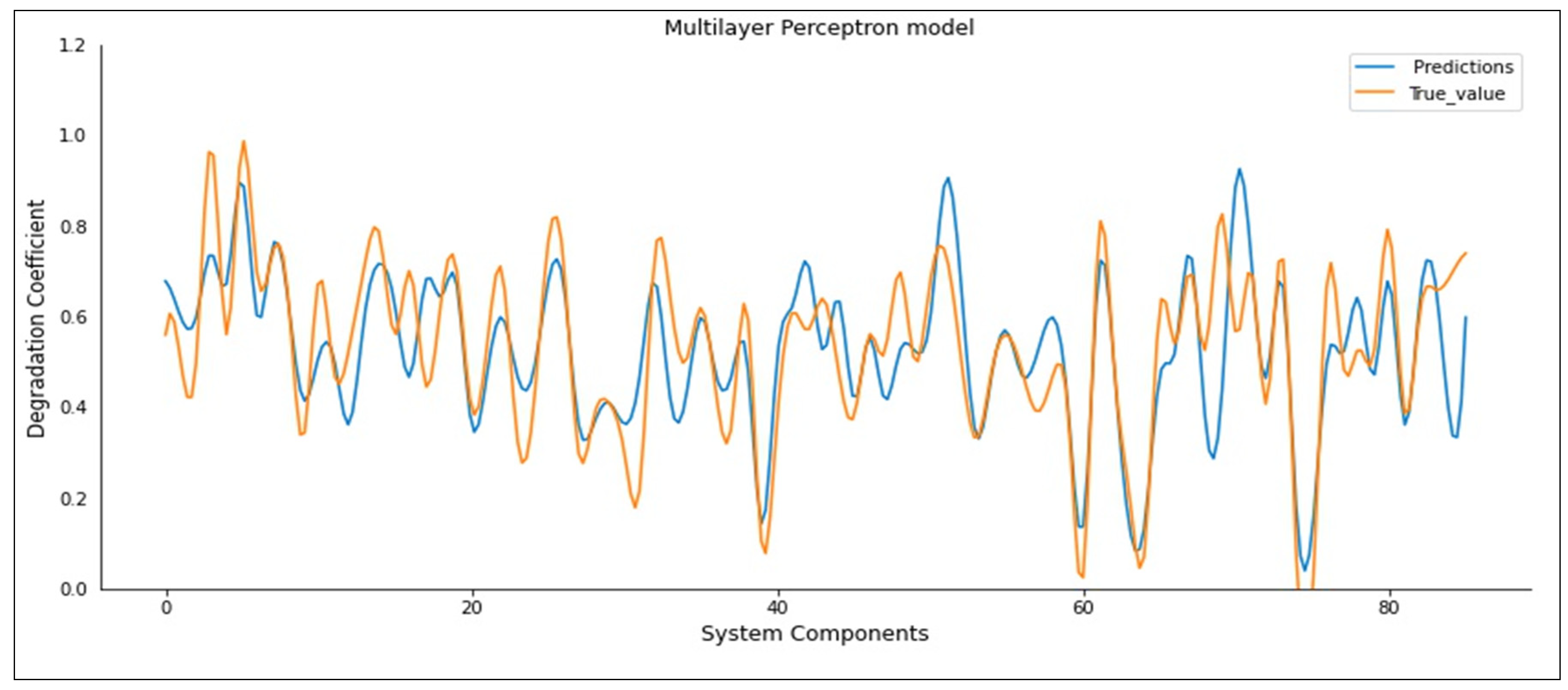
To assess the model’s effectiveness in predicting the degradation coefficient of components post operation, the ‘evaluate’ function is used. This function provides us with both training and evaluation scores based on MSE, MAE, and MAPE loss functions. The simulation results are presented in Table 2 and Figure 2, Figure 3 and Figure 4. Table 2 displays the performance metrics results for the ANN model on the FMS dataset, juxtaposed with other regression models (Support Vector Regression SVR).

Table 2.
Results of performance metrics comparing ANN and SVR models.
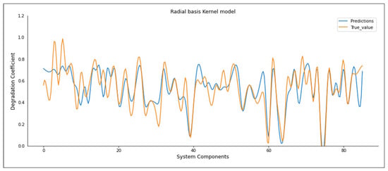
Figure 2.
Actual and predicted degradation coefficient with SVR-RBF Kernel.
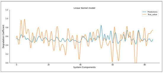
Figure 3.
Actual and predicted degradation coefficient with SVR-Linear Kernel.

Figure 4.
Actual and predicted degradation coefficient with ANN model.
Figure 2 and Figure 3 reveal a significant margin between the actual and predicted values, particularly evident in the SVR with linear kernel model and SVR with RBF Kernel. In contrast, Figure 4 illustrates that the ANN model’s predicted values are closely aligned with the true value, demonstrating a smaller error when compared to the SVR models. This observation is entirely consistent with the results obtained in Table 2, where all accuracy evaluation indices are in favor of the ANN model. Thus, the results obtained revealed that the ANN is more suitable for predicting the degradation coefficient than the different SVR models. Moreover, the constructed model can be used to predict the system’s actual age based on its maintenance data.
4.3. Selective Maintenance with Multi-Strategies
Due to machine degradation, the failure rates increase, and the maintenance operation plays a crucial role in both eliminating the effects of this degradation and improving the overall system age. As perfect maintenance incurs significant expenses, in this context, we consider the possibility of implementing multi-level maintenance activities to effectively reduce both maintenance costs and time. In this context, we posit that maintenance action proportionally enhances the component’s age compared to its state before the maintenance activity. The impact of maintenance actions on the component’s age is expressed by the following equation:
where is the age improvement value. for or before maintenance operation and is the age after maintenance operation with .
4.3.1. Optimization Model
The decision variables are
The total maintenance cost is the sum of the maintenance costs of individual components which depends on the selected maintenance strategy . Therefore, the selective maintenance optimization problem can be formulated as follows:
Subject to:
The objective Function (22) aims to minimize the total maintenance cost. Constraint (23) calculates the remaining useful life of component after performing mission . Constraint (24) calculates the real age of component at the end of mission . Constraint (25) ensures that the total time of all maintenance actions performed does not exceed the limited intermission break time. Constraint (26) indicates that only one maintenance strategy can be performed on component . Constraint (27) defines that the reliability of the multi-component system for the mission must be at least equal to a reliability threshold fixed by the production stakeholders. Constraint (28) defines that decision variables are binary.
4.3.2. Resolution Method
To solve the problem by determining an optimal maintenance plan, a metaheuristic algorithm based on the extended deluge algorithm was implemented. The extended great deluge is a local search metaheuristic that iteratively repeats the replacement of a current solution by a new one , until some stopping condition has been satisfied. The new solution is selected from a neighborhood [44]. The concept of accepting or rejecting the candidate solution from the neighborhood is different from other methods. In the extended great deluge approach, the algorithm accepts every solution whose objective function is less or equal to the upper limit , which is monotonically increased during the search by .
5. Numerical Results
This section showcases the application of the proposed approach in a case study involving a Flexible Manufacturing System (FMS). Recall that the objective is to establish the optimal maintenance actions at each breakdown using the ANN regression model to predict the component’s real age and then apply the extended deluge metaheuristic algorithm. Also, the selective maintenance decision for the FMS study case involves selecting the optimal number of components to be maintained, while minimizing the total maintenance cost and adhering to a reliability threshold (see the optimization model in Section 5.2).
Hence, the FMS components encompass diverse assembly configurations, with some arranged in series and others in parallel. The proposed methodology, leveraging machine learning and optimization techniques, is applicable to any system component structure (multi-series parallel). In contrast, the assessment of system reliability involves computing the reliability of these components, considering their respective structures. Equation (29) is utilized for series structures, while Equation (30) is applied for parallel structures. It is worth noting that the reliability of component , denoted as .
5.1. FMS Study Case and Input Data
The Flexible Manufacturing System situated in the Laboratory of Computer Engineering, Production, and Maintenance (LGIPM) serves the dual purpose of research and teaching. We assume that the specific maintenance periods throughout the year align with five educational breaks, as illustrated in Figure 5. The selection of the number of maintenance actions is primarily influenced by the availability of service technicians. As a result, a multi-level selective maintenance approach is highly recommended for the FMS during each scheduled downtime.

Figure 5.
The missions and breakdowns of FMS.
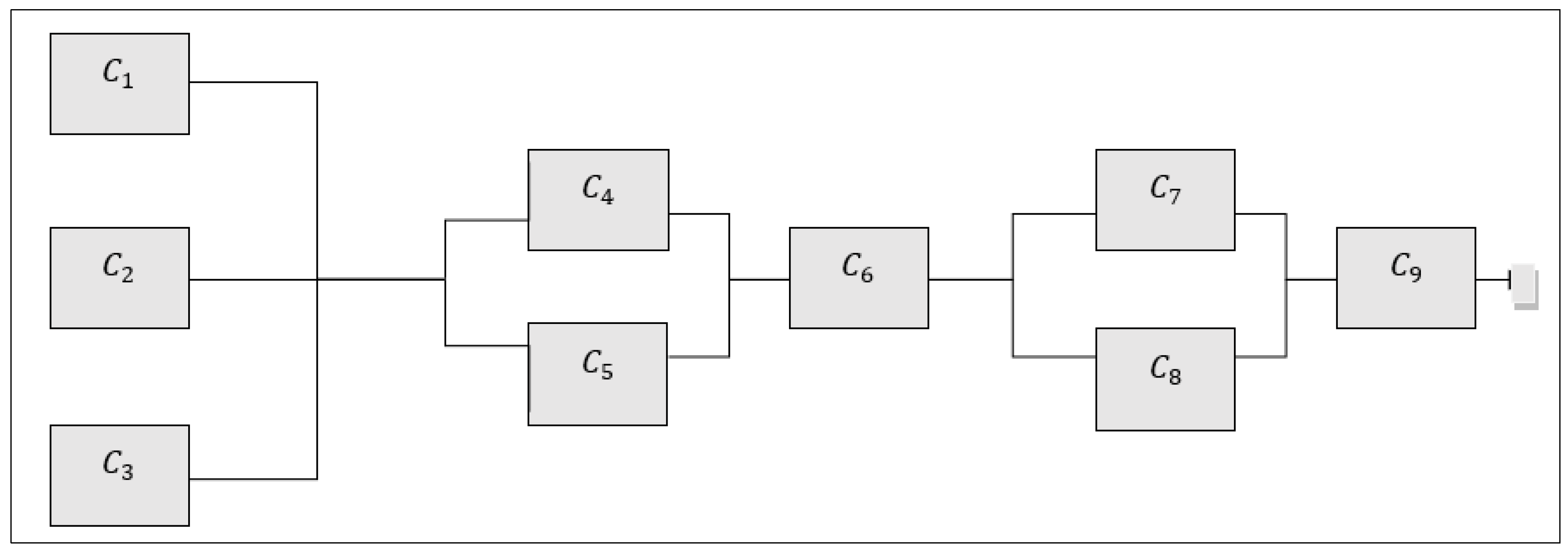
Given the extensive array of components in the FMS, encompassing electrical, electronic, and mechanical elements totaling around 300,000, we have opted to focus on a multi-series parallel subsystem. This subsystem of the FMS consists of nine components (), as shown in Figure 6, and serves as the basis for developing our proposed methodology.
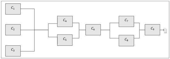
Figure 6.
The FMS structure.
As explained through this paper, we adopt multi-level selective maintenance in which each level proportionally improves the component’s age compared to its value before maintenance activity as well as its reliability. In addition, each level is characterized by its cost and time duration, as detailed in Table 3. The theoretical age given by the manufacturer () for each component is defined in the second column. Note that, for the illustrative example, we have opted for a choice among five maintenance levels, starting from the first level (), which involves no action, to the final level (), which includes the replacement of the component. At each breakdown, the maintenance plan must ensure the fulfillment of the subsequent mission with a reliability level exceeding or equal to ().

Table 3.
Parameters of multi-level maintenance for each component.
5.2. Results
By exploiting the ANN model, we predict, firstly, the degradation factor at every breakdown () for each component (). Then, based on experiment results and utilizing Equation (24), we establish the actual age for each component. These results are illustrated in Table 4. We observe a slight degradation in the components at the end of the first mission (), and this increases with subsequent missions.

Table 4.
The obtained actual age and degradation factor for each component at the end mission .
Note that the results obtained in Table 4 are raw, i.e., without the implementation of maintenance strategies and optimization model at each break. Indeed, our predictive model updates these parameters after each maintenance plan adopted during a given break. The EDA approach on MATLAB 2022 software to address the challenge of proposing a maintenance plan that minimizes costs under reliability and time constraints by using the results of ANN-based predictive model generates the solutions presented in Table 5.

Table 5.
The multi-level maintenance plan obtained for the required reliability level (0.9).
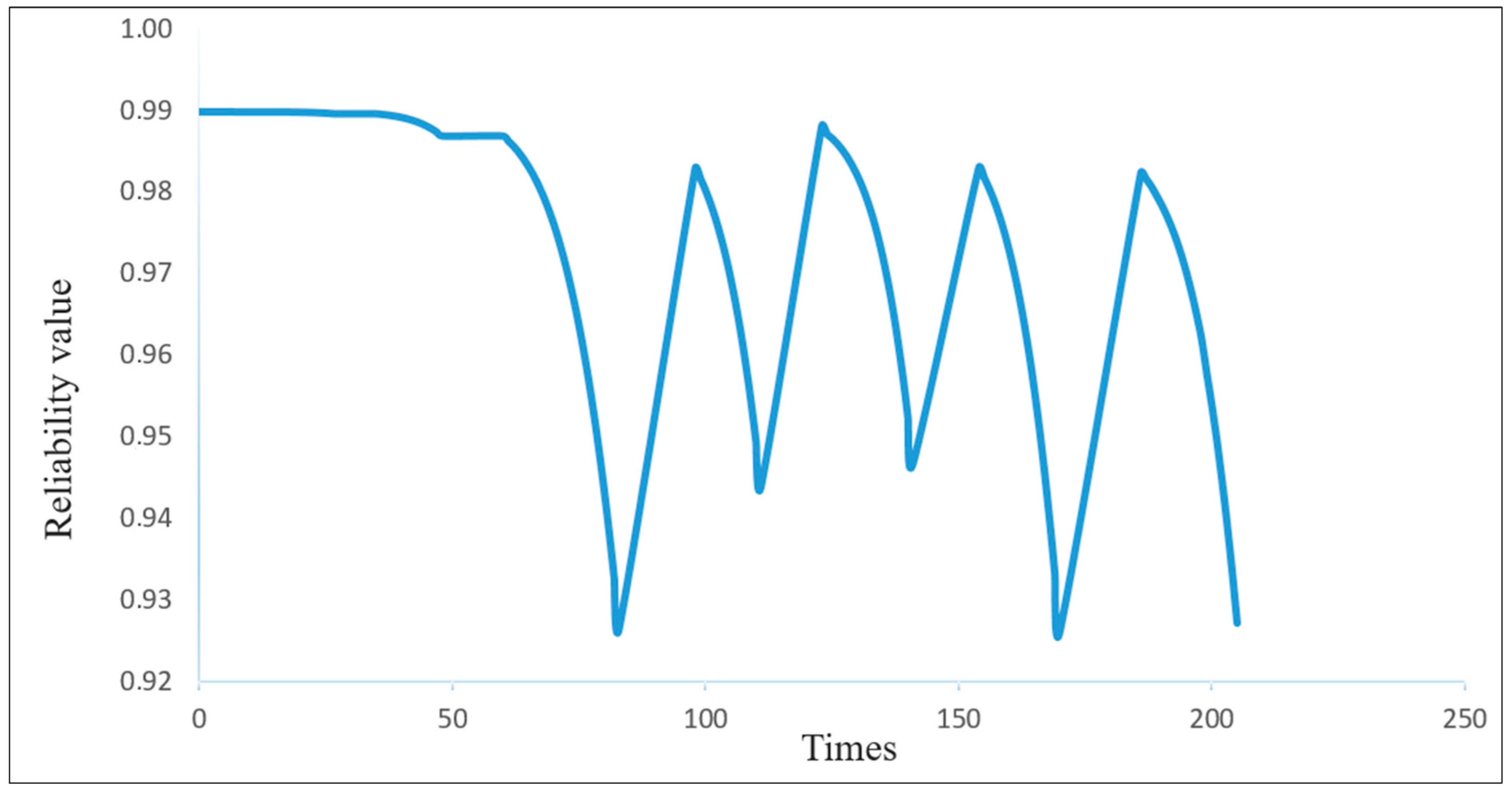
As shown in the table, the actual predicted age of the components is quite high after performing the three first missions (until ), so the best maintenance strategy selected for the nine components during the breaks , and is , which means doing nothing for all components (, ). After accomplishing the fourth mission (), some components are deteriorated and, consequently, the reliability system decreases. By minimizing the total maintenance cost under reliability and time constraints, the best maintenance policy recommended involves implementing strategy 2 on component 1 (), strategy 2 on component 5 (), strategy 3 on component 6 (), strategy 3 on component 8 (), and employing strategy 1 for the remaining components. Following this multi-level maintenance plan, the age of component 1 is increased by (time units), and component 5 is increased by , component 6 by , component by , while no action is performed on the other components. The optimal policy results in a total maintenance cost of (monetary units), a total maintenance time of , and aims to achieve a reliability value equal to .
The obtained maintenance plan during the considered operating time shows that the system reliability decreases during each mission. In order to maintain the system reliability higher than 0.9, the maintenance action selected at the end of the mission allows us to increase the component’s actual age as well as the reliability system; this increase is presented in Figure 7 by an increasing line. Otherwise, the system reliability follows an exponential variation during the operating time. As shown in Figure 7, the maintenance action suggested by the proposed approach during the intermission break ensures that the system’s reliability respects the set threshold until the end of the mission.

Figure 7.
Evolution of system reliability after performing maintenance actions.
6. Conclusions
This paper proposed a predictive model for selective maintenance decision making using machine learning models and mathematical programming. After conducting tests and comparing various machine learning methods, we observed that the ANN, SVR with linear kernel function and SVR with RBF Kernel methods stand out for their reliability in terms of prediction accuracy for selective maintenance. In this paper, these three machine learning models were compared on the provided dataset, and the ANN yielded the highest prediction score. Moreover, at the end of each mission, the constructed model predicts the real age of each component according to the system data collected during the previous operations. Then, multi-level maintenance actions can be performed in order to improve the actual age system and avoid equipment failure, while minimizing the total maintenance cost under time and reliability constraints. In this study, we considered that the selective maintenance strategies depend on the actual conditions of each component, i.e., a low actual age due to degradation phenomena and operating conditions requires a costlier maintenance strategy that strongly improves the age and compensates the degradation effect. To illustrate the robustness of the proposed strategy, a historical maintenance data of the FMS real study was explored to determine a selective maintenance plan. The obtained results show that the proposed model can be used in several industrial fields and help decision-makers determine the best maintenance policy to perform during each intermission break which guarantees the completion of the next operation with a high system reliability.
For the prediction model, future work can focus on a more complex configuration system taking into account the factors of time and environmental conditions (temperature, pressure, humidity, etc.) and implement more ideas using artificial neural networks and machine learning techniques to estimate the probability of the system failure. Subsequently, integrate this probability assessment into the optimization problem and maintenance planning. Also, it is an interesting perspective to integrate other learning methods such as CMFIRL (completely mode-free integral reinforcement learning) [45] and policy iteration (PI) algorithm, by using the technique of neural network linear differential inclusion (LDI) [46] with our joint production and maintenance problem.
Author Contributions
Writing—original draft, A.A.; Writing—review & editing, M.A.K.; Supervision, Z.H. All authors have read and agreed to the published version of the manuscript.
Funding
This research received no external funding.
Institutional Review Board Statement
Not applicable.
Informed Consent Statement
Not applicable.
Data Availability Statement
The data presented in this study are available on request from the corresponding author. The data are not publicly available due to data confidentiality.
Conflicts of Interest
The authors declare no conflict of interes.
Notations
The following notations:
| M | Total maintenance cost during the break between missions and |
| Maintenance level (or strategy) for component with | |
| Cost of the maintenance level | |
| Duration of the maintenance level of component | |
| Maintenance cost per time unit | |
| Cost of assembly\disassembly incurred if at least one component is maintained | |
| Duration of mission | |
| Break duration between mission and | |
| Degradation factor of component at the end of mission | |
| Theoretical component’s age given by the manufacturer | |
| Theoretical remaining useful life of component after performing mission | |
| Actual age of component at the end of the mission | |
| System reliability related to actual ages of multi-components. | |
| Minimal required reliability | |
| Total number of missions |
References
- Duan, C.; Deng, C.; Gong, Q.; Wang, Y. Optimal failure mode-based preventive maintenance scheduling for a complex mechanical device. Int. J. Adv. Manuf. Technol. 2018, 95, 2717–2728. [Google Scholar] [CrossRef]
- Jamshidi, R.; Esfahani, M.M.S. Maintenance policy determination for a complex system consisting of series and cold standby system with multiple levels of maintenance action. Int. J. Adv. Manuf. Technol. 2015, 78, 1337–1346. [Google Scholar] [CrossRef]
- Duan, C.; Deng, C.; Wang, B. Optimal multi-level condition-based maintenance policy for multi-unit systems under economic dependence. Int. J. Adv. Manuf. Technol. 2017, 91, 4299–4312. [Google Scholar] [CrossRef]
- Cao, W.; Jia, X.; Hu, Q.; Zhao, J.; Wu, Y. A literature review on selective maintenance for multi-unit systems. Qual. Reliab. Eng. Int. 2018, 34, 824–845. [Google Scholar] [CrossRef]
- Zhu, H.; Liu, F.; Shao, X.; Liu, Q.; Deng, Y. A cost-based selective maintenance decision-making method for machining line. Qual. Reliab. Eng. Int. 2011, 27, 191–201. [Google Scholar] [CrossRef]
- Nguyen, K.T.; Medjaher, K. A new dynamic predictive maintenance framework using deep learning for failure prognostics. Reliab. Eng. Syst. Saf. 2019, 188, 251–262. [Google Scholar] [CrossRef]
- Asadzadeh, S.; Azadeh, A. An integrated systemic model for optimization of condition-based maintenance with human error. Reliab. Eng. Syst. Saf. 2014, 124, 117–131. [Google Scholar] [CrossRef]
- Murphy, K.P. Machine Learning: A Probabilistic Perspective; MIT Press: Cambridge, MA, USA, 2012. [Google Scholar]
- Najafabadi, M.M.; Villanustre, F.; Khoshgoftaar, T.M.; Seliya, N.; Wald, R.; Muharemagic, E. Deep learning applications and challenges in big data analytics. J. Big Data 2015, 2, 1. [Google Scholar] [CrossRef]
- Rice, W.F.; Cassady, C.R.; Nachlas, J.A. Optimal maintenance plans under limited maintenance time. In Proceedings of the Seventh Industrial Engineering Research Conference, Banff, AB, Canada, 9–10 May 1998; pp. 1–3. [Google Scholar]
- Cassady, C.R.; Murdock, W.P., Jr.; Pohl, E.A. Selective maintenance for support equipment involving multiple maintenance actions. Eur. J. Oper. Res. 2001, 129, 252–258. [Google Scholar] [CrossRef]
- Cassady, C.R.; Pohl, E.A.; Murdock, W.P. Selective maintenance modeling for industrial systems. J. Qual. Maint. Eng. 2001, 7, 104–117. [Google Scholar] [CrossRef]
- Djelloul, I.; Khatab, A.; Aghezzaf, E.H.; Sari, Z. Optimal selective maintenance policy for series-parallel systems operating missions of random durations. In Proceedings of the International Conference on Computers & Industrial Engineering (CIE 45), Metz, France, 28–30 October 2015; pp. 28–30. [Google Scholar]
- Pandey, M.; Zuo, M.J.; Moghaddass, R. Selective maintenance modeling for a multistate system with multistate components under imperfect maintenance. IIE Trans. 2013, 45, 1221–1234. [Google Scholar] [CrossRef]
- Meng, M.H.; Zuo, M.J. Selective maintenance optimization for multi-state systems. In Proceedings of the Engineering Solutions for the Next Millennium. 1999 IEEE Canadian Conference on Electrical and Computer Engineering (Cat. No. 99TH8411), Edmonton, AB, Canada, 9–12 May 1999; Volume 3, pp. 1477–1482. [Google Scholar]
- Pandey, M.; Zuo, M.J.; Moghaddass, R. Selective maintenance for binary systems using age-based imperfect repair model. In Proceedings of the 2012 International Conference on Quality, Reliability, Risk, Maintenance, and Safety Engineering (QR2MSE), Chengdu, China, 15–18 June 2012; pp. 385–389. [Google Scholar]
- Khatab, A.; Aghezzaf, E.-H. Selective maintenance optimization when quality of imperfect maintenance actions are stochastic. Reliab. Eng. Syst. Saf. 2016, 150, 182–189. [Google Scholar] [CrossRef]
- Martorell, S.; Sánchez, A.; Carlos, S.; Serradell, V. Simultaneous and multi-criteria optimization of TS requirements and maintenance at NPPs. Ann. Nucl. Energy 2002, 29, 147–168. [Google Scholar] [CrossRef]
- Khatab, A.; Diallo, C.; Aghezzaf, E.-H.; Venkatadri, U. Condition-based selective maintenance for stochastically degrading multi-component systems under periodic inspection and imperfect maintenance. Proc. Inst. Mech. Eng. Part O J. Risk Reliab. 2018, 232, 447–463. [Google Scholar] [CrossRef]
- Han, X.; Wang, Z.; Xie, M.; He, Y.; Li, Y.; Wang, W. Remaining useful life prediction and predictive maintenance strategies for multi-state manufacturing systems considering functional dependence. Reliab. Eng. Syst. Saf. 2021, 210, 107560. [Google Scholar] [CrossRef]
- Benkedjouh, T.; Medjaher, K.; Zerhouni, N.; Rechak, S. Remaining useful life estimation based on nonlinear feature reduction and support vector regression. Eng. Appl. Artif. Intell. 2013, 26, 1751–1760. [Google Scholar] [CrossRef]
- Bengio, Y.; Courville, A.; Vincent, P. Representation learning: A review and new perspectives. IEEE Trans. Pattern Anal. Mach. Intell. 2013, 35, 1798–1828. [Google Scholar] [CrossRef] [PubMed]
- Li, C.; Sánchez, R.V.; Zurita, G.; Cerrada, M.; Cabrera, D.; Vásquez, R.E. Gearbox fault diagnosis based on deep random forest fusion of acoustic and vibratory signals. Mech. Syst. Signal Process. 2016, 76–77, 283–293. [Google Scholar] [CrossRef]
- He, Z.; Shao, H.; Ding, Z.; Jiang, H.; Cheng, J. Modified Deep Autoencoder Driven by Multisource Parameters for Fault Transfer Prognosis of Aeroengine. IEEE Trans. Ind. Electron. 2021, 69, 845–855. [Google Scholar] [CrossRef]
- Chen, C.; Wang, C.; Lu, N.; Jiang, B.; Xing, Y. A data-driven predictive maintenance strategy based on accurate failure prognostics. Eksploat. I Niezawodn.-Maint. Reliab. 2021, 23, 387–394. [Google Scholar] [CrossRef]
- Shoorkand, H.D.; Nourelfath, M.; Hajji, A. A hybrid CNN-LSTM model for joint optimization of production and imperfect predictive maintenance planning. Reliab. Eng. Syst. Saf. 2023, 241, 109707. [Google Scholar] [CrossRef]
- Zheng, P.; Zhao, W.; Lv, Y.; Qian, L.; Li, Y. Health Status-Based Predictive Maintenance Decision-Making via LSTM and Markov Decision Process. Mathematics 2023, 11, 109. [Google Scholar] [CrossRef]
- Zonta, T.; da Costa, C.A.; Zeiser, F.A.; Ramos, G.d.O.; Kunst, R.; Righi, R.d.R. A predictive maintenance model for optimizing production schedule using deep neural networks. J. Manuf. Syst. 2022, 62, 450–462. [Google Scholar] [CrossRef]
- Deutsch, J.; He, D. Using deep learning-based approach to predict remaining useful life of rotating components. IEEE Trans. Syst. Man Cybern. Syst. 2017, 48, 11–20. [Google Scholar] [CrossRef]
- Dargan, S.; Kumar, M.; Ayyagari, M.R.; Kumar, G. A survey of deep learning and its applications: A new paradigm to machine learning. Arch. Comput. Methods Eng. 2020, 27, 1071–1092. [Google Scholar] [CrossRef]
- Namuduri, S.; Narayanan, B.N.; Davuluru, V.S.P.; Burton, L.; Bhansali, S. Review—Deep learning methods for sensor based predictive maintenance and future perspectives for electrochemical sensors. J. Electrochem. Soc. 2020, 167, 037552. [Google Scholar] [CrossRef]
- Kammoun, M.A.; Rezg, N. Toward the optimal selective maintenance for multi-component systems using observed failure: Applied to the FMS study case. Int. J. Adv. Manuf. Technol. 2018, 96, 1093–1107. [Google Scholar] [CrossRef]
- Kammoun, M.A.; Hajej, Z.; Rezg, N. A multi-level selective maintenance strategy combined to data mining approach for multi-component system subject to propagated failures. J. Syst. Sci. Syst. Eng. 2022, 31, 313–337. [Google Scholar] [CrossRef]
- Ben-Salem, A.; Gharbi, A.; Hajji, A. Environmental issue in an alternative production–maintenance control for unreliable manufacturing system subject to degradation. Int. J. Adv. Manuf. Technol. 2015, 77, 383–398. [Google Scholar] [CrossRef]
- Bouslah, B.; Gharbi, A.; Pellerin, R. Joint economic design of production, continuous sampling inspection and preventive maintenance of a deteriorating production system. Int. J. Prod. Econ. 2016, 173, 184–198. [Google Scholar] [CrossRef]
- Fan, F.-L.; Xiong, J.; Li, M.; Wang, G. On interpretability of artificial neural networks: A survey. IEEE Trans. Radiat. Plasma Med Sci. 2021, 5, 741–760. [Google Scholar] [CrossRef] [PubMed]
- Abiodun, O.I.; Jantan, A.; Omolara, A.E.; Dada, K.V.; Umar, A.M.; Linus, O.U.; Arshad, H.; Kazaure, A.A.; Gana, U.; Kiru, M.U. Comprehensive review of artificial neural network applications to pattern recognition. IEEE Access 2019, 7, 158820–158846. [Google Scholar] [CrossRef]
- Feng, J.; Lu, S. Performance Analysis of Various Activation Functions in Artificial Neural Networks. J. Phys. Conf. Ser. 2019, 1237, 022030. [Google Scholar] [CrossRef]
- Apicella, A.; Donnarumma, F.; Isgrò, F.; Prevete, R. A survey on modern trainable activation functions. Neural Netw. 2021, 138, 14–32. [Google Scholar] [CrossRef]
- Yan, M.; Wang, X.; Wang, B.; Chang, M.; Muhammad, I. Bearing remaining useful life prediction using support vector machine and hybrid degradation tracking model. ISA Trans. 2020, 98, 471–482. [Google Scholar] [CrossRef] [PubMed]
- Cortes, C.; Vapnik, V. Support-vector networks. Mach. Learn. 1995, 20, 273–297. [Google Scholar] [CrossRef]
- Bergstra, J.; Bengio, Y. Random search for hyper-parameter optimization. J. Mach. Learn. Res. 2012, 13, 281–305. [Google Scholar]
- Zhang, Z. Improved adam optimizer for deep neural networks. In Proceedings of the 2018 IEEE/ACM 26th International Symposium on Quality of Service (IWQoS), Banff, AB, Canada, 4–6 June 2018; pp. 1–2. [Google Scholar]
- Acan, A.; Ünveren, A. Multiobjective great deluge algorithm with two-stage archive support. Eng. Appl. Artif. Intell. 2020, 87, 103239. [Google Scholar] [CrossRef]
- Fang, H.; Zhang, M.; He, S.; Luan, X.; Liu, F.; Ding, Z. Solving the Zero-Sum Control Problem for Tidal Turbine System: An Online Reinforcement Learning Approach. IEEE Trans. Cybern. 2022, 53, 7635–7647. [Google Scholar] [CrossRef]
- He, S.; Fang, H.; Zhang, M.; Liu, F.; Ding, Z. Adaptive optimal control for a class of nonlinear systems: The online policy iteration approach. IEEE Trans. Neural Netw. Learn. Syst. 2019, 31, 549–558. [Google Scholar] [CrossRef]
Disclaimer/Publisher’s Note: The statements, opinions and data contained in all publications are solely those of the individual author(s) and contributor(s) and not of MDPI and/or the editor(s). MDPI and/or the editor(s) disclaim responsibility for any injury to people or property resulting from any ideas, methods, instructions or products referred to in the content. |
© 2023 by the authors. Licensee MDPI, Basel, Switzerland. This article is an open access article distributed under the terms and conditions of the Creative Commons Attribution (CC BY) license (https://creativecommons.org/licenses/by/4.0/).

