Abstract
RRT (rapidly exploring random tree) is a sampling-based planning algorithm that has been widely used due to its simple structure and fast speed. However, the RRT algorithm has several issues such as low planning efficiency, high randomness, and poor path quality. To address these issues, this paper proposes a novel method, the adjustable probability and sampling area and the Dijkstra optimization-based RRT algorithm (APSD-RRT), which consists of the following two modules: an APS-RRT planner and an optimizer. The APS-RRT planner can reach a feasible path quickly using the proposed adjustable probability and sampling area strategies, while the optimizer applies the Dijkstra algorithm to prune and improve the initial path generated by the APS-RRT planner and smooths-out sharp nodes based on the interpolation method. A series of experiments are conducted to demonstrate that our method can perform much better in terms of the balance between the computing cost and performance.
1. Introduction
Path planning is the problem of finding a safe path from an initial state to a target state in a given area and selecting an optimal scheme based on evaluation indicators such as path distance and planning time [1,2]. Path planning is a key technology in the fields of robotics, drones, autonomous driving, etc., and has attracted widespread attention from researchers [3].
In the past few decades, many path-planning algorithms have been proposed, such as the graph-based A* algorithm [4], the artificial potential field (APF) algorithm [5], the genetic algorithm (GA) [6,7], the sampling-based probabilistic road map (PRM) algorithm [8], etc. The A* algorithm is an effective method for solving the shortest-path problem, but its performance depends on the grid size of the resolution. The A* algorithm has an exponential increasement in computing cost when an environment is complex. The APF algorithm constructs a virtual force field to realize real-time path planning, but it is easy to fall into a local optimum. The GA optimizes populations of candidate solutions using selection, crossover, and mutation operations to find an optimal solution, but it has a problem of premature convergence. The PRM algorithm constructs a roadmap by sampling in the configuration space and then searches for a path using graph search methods, but it relies on the quality of the samples.
The RRT algorithm [9] builds a search tree by sampling randomly in the configuration space. Compared to traditional path-planning algorithms, the RRT algorithm can find a feasible path without complex environment modeling and handle high-dimensional complex situations. However, the RRT algorithm cannot guarantee the quality of the path. Karaman et al. [10] proposed the RRT* algorithm to solve this issue, which considers the cost of neighboring states after each successful expansion and uses Choose-Parent and Rewire strategies to modify the connection between a new state and its neighbors. The RRT* algorithm has been proven to be asymptotically optimal, as it can reach an optimal solution when the number of samples go to infinity, but it takes a lot of time. In other words, RRT* is an algorithm that trades computing cost for performance. The crucial reason for the inefficiency of the RRT* algorithm is that the entire search tree needs to be traversed when a state is inserted into the tree. As the number of states increases, the cost of traversing the tree each time becomes huge.
To accelerate the convergence process of the RRT* algorithm, in [11], the Informed-RRT* algorithm introduces an ellipsoidal heuristic set, in which the current best solution is used as the major axis of the ellipse, and the initial state and target state are treated as the focus of the ellipse, which can restrict the sampling process to this set. As better solutions are found, the heuristic set is reduced gradually. It greatly reduces unnecessary explorations in these regions where the solution probably does not exist. However, the quality of the initial path has a decisive influence on the performance of the algorithm. In the worst situation, the Informed-RRT* algorithm equals the RRT* algorithm in performance. Nasir et al. [12] proposed the RRT*-smart algorithm using the idea of triangle inequality to optimize the path after finding the solution and then taking bias sampling to high-quality nodes. As the name suggests, this algorithm selects sampling nodes more purposefully, but it also faces the same issue as the Informed-RRT*. Wu et al. [13] presented the Fast-RRT algorithm, which increases the speed of searching for the optimal path by fusing the current solution with the best solution continuously, but this algorithm cannot guarantee to achieve the optimal solution.
Recently, some post-processing methods have been used in path optimization. The advantage of these methods is that they have no impact on the performance of the planner while improving the quality of the path within an acceptable time. In [14], the improved particle swarm optimization (PSO) algorithm is utilized to optimize the key nodes after finding the initial path. Similarly, in [15], a set of paths is treated as a population, and the GA is utilized to calculate the optimal solution. However, these methods have some parameters that need to be set in advance.
The RRT algorithm uses a uniform sampling strategy to explore the whole configuration space; this process is random and inefficient. In other words, the samples are selected without purpose, as most of them have no impact on the final path. In order to make the exploration more efficient, in [16], the RRT-Connect algorithm is proposed, which grows two trees from the initial and target states alternately and combines a greedy strategy to enhance the algorithm’s speed, but it still applies the uniform sampling strategy. In [17], the Bias-RRT algorithm chooses a target state as the sample with a certain probability to guide the tree to reach the goal quickly, but it is easy to fall into a local minimum using this strategy. The 1-0 Bg-RRT algorithm [18] is an enhanced version of the Bias-RRT algorithm, in which the goal bias probability is changed by two values, 0 and 1. Although the algorithm’s performance in simple situations has been improved to some extent, it still retains the same issues in complex situations. Chai et al. [19] introduced the greedy sampling space reduction and environmental judgment strategies that can handle complex scenarios such as narrow passages, but their algorithm lacks stability.
In combination with other algorithms, in [20], the authors combined the potential field idea of the APF algorithm to guide the expansion process of the RRT algorithm, keeping the path away from obstacles, but there is obvious oscillation in the path. Wang et al. [21] used the generalized voronoi graph (GVG) to find the initial path and then applied the multiple potential functions (MPF) to generate a non-uniform distribution for guiding the sampling process. However, their algorithm faces challenges, as the GVG takes a lot of time to find the initial path in complex scenarios.
Learning-based methods have become popular in recent years. In [22], a neural network was trained to replicate human decision making to drive a mobile robot in uncertain scenarios. Ichter et al. [23] trained a conditional variational autoencoder (CVAE) model to predict non-uniform sampling from latent space. Li et al. [24] utilized a neural network to predict cost functions and solve motion planning problems with kinodynamic constraints. Wang et al. [25] applied a convolutional neural network (CNN) model, using the A* algorithm planning cases as the dataset, to predict the optimal path distribution in an environment. Learning-based methods have good scalability and show some promising prospects, but the success of these methods depends on the quality of the dataset. There is still plenty of room for improvement in terms of the performance of the model.
All of these points indicate that algorithms used to generate optimal paths require significant computing resources, while the algorithms used to generate paths quickly cannot guarantee the quality of the path. Moreover, many algorithms exhibit low efficiency in some complex environments. In practical applications, planning algorithms are often required to be able to quickly find solutions in different environments while meeting certain quality requirements. The balance between the computing cost and performance is a key consideration of this work. To overcome this issue, we proposed the APSD-RRT method, which is a two-stage algorithm. In the first stage, the planner is designed to quickly achieve a feasible solution using adjustable probability and sampling area strategies. In the second stage, the optimizer is designed to enhance the quality of the path generated by the planner; it is equipped with the Dijkstra pruning and interpolation strategies. The combination of the planner and the optimizer shows excellent results in terms of the balance between the computing cost and performance.
The rest of this article is organized as follows. The definitions of the path planning problem and the basic RRT algorithm are reported in Section 2. The proposed methods are introduced in Section 3. The simulation results and analysis are presented in Section 4. Finally, we present our conclusions in Section 5.
2. Background
In Section 2.1 and Section 2.2, respectively, the definition of the path planning problem and the basic premises of the RRT algorithm are introduced.
2.1. Problem Definition
Let be the configuration space of the path planning task, and d be the dimension of the configuration space. represents the impassable obstacle area. represents the free area that can be traversed. is the initial state, and is the target state. If there is a collision-free path between the two nodes and , let a continuous function represent this path. Let f(η) be the Euclidean distance cost function of the path η, such that:
Two important questions are defined as follows:
Problem 1 (Feasible Path Planning): the feasible planning task involves finding a collision-free path, , connecting xinit and xgoal, such that and . If the path is not found within the given time, an error is reported.
Problem 2 (Optimal Path Planning): let ∑ be the set of feasible paths. The optimal planning task is to find a path η* with the lowest distance cost, connecting xinit and xgoal, within the given time, such that .
2.2. Basic RRT Algorithm
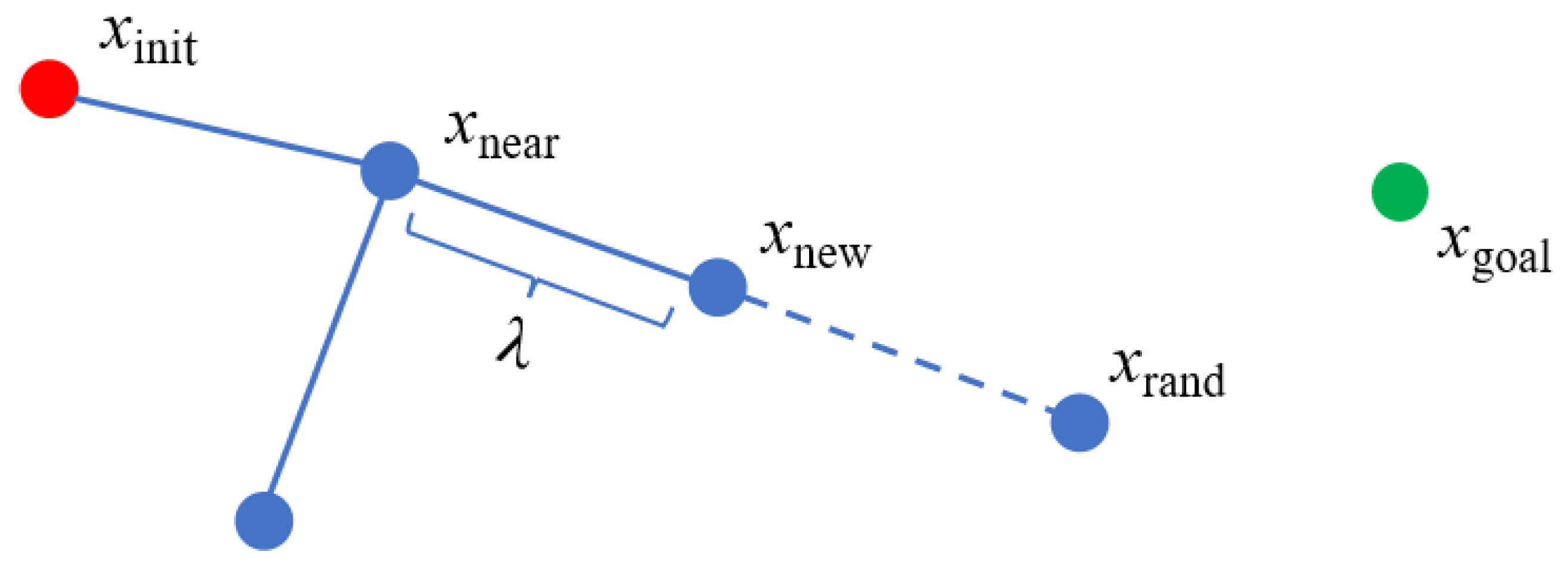
The RRT algorithm builds a search tree by sampling randomly in the configuration space. Let the initial state xinit be the root node of the tree. Then, the following steps are followed until a path is found or the maximum number of iterations is reached: (1) A state xrand is sampled in the configuration space using the uniform distribution strategy (line 3 in Algorithm 1). (2) A state xnear that is closest to xrand in the tree is found (line 4 in Algorithm 1). (3) A certain step size λ is expanded from xnear to xrand and a new state xnew is obtained (line 5 in Algorithm 1). (4) If the edge {xnear, xnew} is free of collisions, then xnew and the edge {xnear, xnew} are added to the tree (line 6–8 in Algorithm 1). Otherwise, this expansion is discarded and the process returns to Step (1). If the search tree achieves the target region , xnew and xgoal are connected and returned to the path (line 9–11 in Algorithm 1). If no path is found after the maximum number of iterations, the planning fails. Figure 1 illustrates the expansion process of RRT.
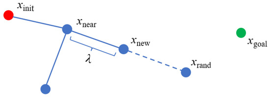
Figure 1.
The expansion process of the RRT algorithm. The new state xnew is inserted into the search tree.
| Algorithm 1. RRT |
| Input: xinit, xgoal and Map Output: A feasible path η from xinit to xgoal 1: Tree.init() 2: for i = 1 to N do 3: xrand ← UniformSample(Map) 4: xnear ← Near(xrand, Tree) 5: xnew ← Steer(xrand, xnear, λ) 6: if CollisionFree(xnear, xnew, Map) then 7: Tree.AddNode(xnew) 8: Tree.AddEdge(xnear, xnew) 9: if xnew ∈ Xgoal then 10: return η 11: end 12: end 13: end |
3. Methods
In this section, we discuss the proposed APSD-RRT method, which consists of two modules: the APS-RRT planner and optimizer. Figure 2 shows the overall architecture of the APSD-RRT algorithm. Let the 2D image be the configuration space; it is denoted as Map, where the black and white areas indicate the obstacles and free space, respectively. The initial and target states are marked by red and green points, respectively. The input (Map, xinit, Xgoal) is fed into the planner. The initial path marked with red lines is calculated by the APS-RRT planner (line 2 in Algorithm 2). The optimizer then takes the initial output as its input. It first obtains the key nodes in the initial path using the Dijkstra pruning strategy and then smooths out sharp nodes in the path using the interpolation strategy. Finally, it outputs the improved results, which are marked with dark blue lines. If the initial path does not exist, an error is reported. (line 3–7 in Algorithm 2).
| Algorithm 2. APSD-RRT |
| Input: xinit, xgoal and Map Output: A path η* from xinit to xgoal 1: Map.init 2: ηinit ← Planner(xinit, xgoal, Map) 3: if ηinit exist then 4: η* ← Optimizer(ηinit) 5: else 6: return Failure 7: end |
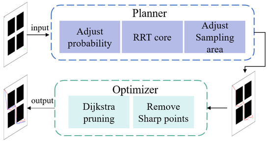
Figure 2.
The framework of the proposed APSD-RRT algorithm.
3.1. APS-RRT Planner
In this section, two important improvements to the sampling process of the RRT algorithm are proposed. First, the uniform sampling strategy is replaced by the adjustable probability strategy, denoted as AP (line 3 in Algorithm 3). Second, the planner checks the growth status of the search tree after each expansion. Once the search tree enters the next-level area, the sampling area is reduced using the adjustable sampling area strategy, denoted as AS (line 12–14 in Algorithm 3). The two strategies are explained in Section 3.1.1 and Section 3.1.2, respectively.
| Algorithm 3. Planner |
| Input: xinit, xgoal and Map; Output: A feasible path ηinit from xinit to xgoal 1: Tree.init() 2: for i = 1 to N do 3: xrand ← AP(Map) 4: xnear ← Near(xrand, Tree) 5: xnew ← Steer(xrand, xnear, λ) 6: if CollisionFree(xnear, xnew, Map) then 7: Tree.AddNode(xnew) 8: Tree.AddEdge(xnear, xnew) 9: if xnew ∈ Xgoal then 10: return ηinit 11: end 12: if flag ! = 2 then 13: Map ← AS(xnew, Map) 14: end 15: end 16: if CannotFindAreaSolution then 17: Tree ← FailSample(Tree, Map) 18: end 19: end |
3.1.1. Adjustable Probability Strategy
The Bias-RRT algorithm uses a fixed probability to expand toward the target state, which reduces the randomness of the expansion process of the RRT algorithm to some extent. However, different goal bias probability values have different levels of adaptability to certain environments. For example, when the environment is relatively sparse, a lower goal bias probability p may slow down the planner’s speed. Clearly, it is more suitable to take a higher goal bias probability value in this case. On the other hand, when there are many obstacles in the environment, a higher goal bias probability p may lead the planner to a local minimum. In this case, it is better to reduce the value of the goal bias probability as far as possible.
Based on the above discussion, the adjustable probability strategy is proposed. This strategy adjusts the value of goal bias probability adaptively, according to the growth status of the tree. When the tree reaches the obstacle area, the goal bias probability decreases adaptively. On the other hand, when the tree arrives at the free area, the goal bias probability increases gradually.
Specifically, at each iteration, the value of p is calculated using Equation (2), where , and pmin and pmax are the lower and upper bounds of the range of p, respectively (line 1 in Algorithm 4). nfail represents the number of failed expansions, and the initial value is set to 0. nsuccess represents the number of successful expansions, and the initial value is set to 1. The expansion success rate is calculated according to . The higher the expansion success rate, the lower the expansion failure rate. The value of the goal bias probability p is adaptively adjusted based on this rate, such that the value of p decreases as nfail increases and increases as nsuccess increases.
A random number between 0 and 1 is generated to determine which sampling strategy to choose. If , the uniform sampling strategy is utilized. Otherwise, the expansion is carried out in the direction of the target state (line 2–6 in Algorithm 4).
| Algorithm 4. AP |
| Input: Map Output: xrand 1: p = pmin + (pmax − pmin) × (nsuccess/nfail + nsuccess) 2: if Rand(0,1) > p then 3: xrand ← UniformSample(Map) 4: else 5: xrand ← xgoal 6: end |
3.1.2. Adjustable Sampling Area Strategy
The RRT algorithm draws samples using the uniform sampling strategy. This process is random and inefficient, leading the algorithm to sample in some useless areas. Moreover, the states in these areas have no effect on the final path, so this sampling strategy not only wastes time but also increases memory usage. To avoid such situations, it is hoped that the sampling nodes are distributed in the promising region where the solutions may exist as much as possible, which means that feasible solutions can be found more quickly. Considering that the RRT algorithm is a single-query incremental method, the configuration space is divided into three level areas, the StartingArea, the MiddleArea, and the TargetArea, according to the positions of the initial state and the target state. For brevity and clarity, StartingArea, MiddleArea, and TargetArea are denoted as S, M and T, respectively. These areas are calculated using Equations (3)–(5), and each area can be treated as a state set, where τi (i = 1, 2, 3, 4) are hyperparameters that represent the boundary of each set. It should be noted that .
Area S equals the global space, where the planner samples the whole space, similarly to the basic RRT algorithm, in the area S. The new state xnew is used to check the growth status of the search tree. When , the search tree is currently in area S (line 1–2 in Algorithm 5). When the search tree arrives at area M, where, the sampling area is reduced from S to M. At this time, the planner only draws samples in area M. In other words, the samples are not generated from area S\M (line 3–4 in Algorithm 5). When the search tree reaches area T, where, the sampling area is reduced from M to T, and the tree searches for the target state in area T (line 5–7 in Algorithm 5). flag is a query variable that has three possible values, 0, 1, and 2, which are used to indicate that the search tree is currently in area S, M, or T, respectively. When the value of flag equals 2, the AS strategy will no longer be executed. By gradually reducing the sampling area, the planner can avoid undertaking unnecessary explorations in unimportant regions, thus improving the planner’s speed.
| Algorithm 5. AS |
| Input: xnew, Map Output: Map, flag 1: if xnew ∈ S\M then 2: Map ← S, flag ← 0 3: else if xnew ∈ M\T then 4: Map ← M, flag ← 1 5: else 6: Map ← T, flag ← 2 7: end |
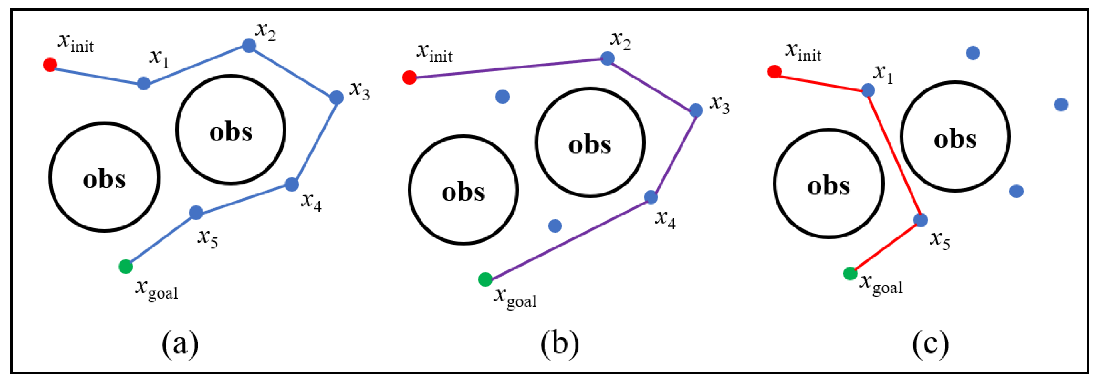
To prevent the algorithm from failing to find a solution due to the limited sampling area strategy, the area’s sampling times are set. If the random tree cannot enter the next area or find the target state within the specified times, the planner is considered to be stuck in a local minimum. At this time, the planner goes to the difference space between the current sampling area and the global sampling area and samples there several times using the FailSample function. The uniform sampling strategy is performed in the FailSample function (line 16–18 in Algorithm 3). It should be noted that, if the planner cannot meet the conditions in area S, the FailSample function is conducted there. After that, the algorithm moves back to the current area to perform several samplings. If the conditions are still not met, the above operations are repeated until they are. Therefore, the improved algorithm can be guaranteed to achieve probabilistically completeness. An example is shown in Figure 3. When states x1 and x2 are added to the tree, this indicates that the search tree has reached areas M and T, respectively. There are obstacles marked with black in area T that prevent the tree from reaching the target state. Even after several samplings, the target state cannot be found in area T, so the FailSample function is applied in area S\T. After several samplings, the planner returns to area T and finally finds the target state in this area.
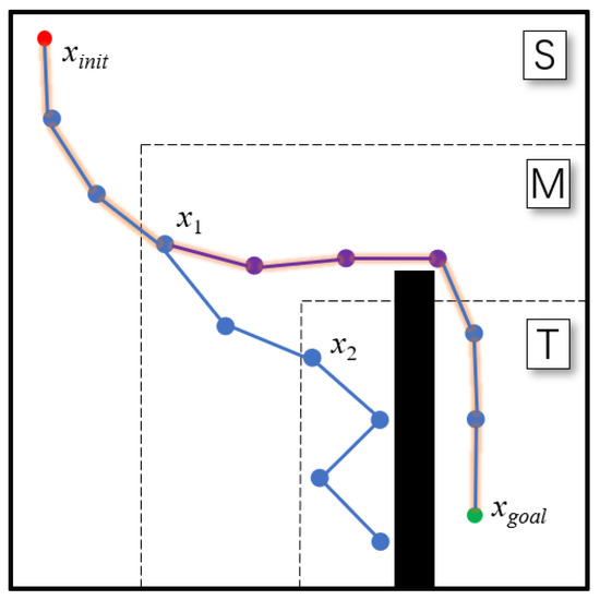
Figure 3.
Illustration of the adjustable sampling area strategy. The nodes added to the tree are marked with blue, and the nodes marked with purple are added to the tree using the FailSample function. The final path is marked with an orange outline.
3.2. Optimizer
In this section, the optimizer module is presented in detail. First, the Dijkstra Pruning strategy is utilized to improve the quality of the initial path generated by the planner (line 2 in Algorithm 6). Second, the Angle function is utilized to calculate each angle in the path, such that
If the angle θ between the two vectors is smaller than the threshold, the Index of the angle is returned and processed using the interpolation strategy. Finally, an improved path is generated (line 3–6 in Algorithm 6). These two strategies are discussed in Section 3.2.1 and Section 3.2.2, respectively.
| Algorithm 6. Optimizer |
| Input: ηinit Output: an optimized path η* 1: Value.init 2: η* ← DijkstraPruning(ηinit,Value) 3: if Angle(η*) < threshold then 4: Index ← Angle(η*) 5: η* ← Interpolation(Index, η*) 6: end |
3.2.1. Dijkstra Pruning
The quality of the path generated by the RRT algorithm is poor; this is mainly reflected in the fact that there are many redundant nodes in the path and the path is relatively tortuous. Generally, this kind of path cannot be directly used in practical applications. In [12], an optimization concept based on triangle inequality is proposed. This method can eliminate redundant nodes and shorten the path length, but it does not find the shortest path based on the current results and there may be issues related to detours, as shown in Figure 4b. Because this method only considers the relationship between three nodes (the child node, the parent node, and the ancestor node) each time, it does not take into account the distance relationship between all the nodes in the path. The Dijkstra algorithm is an effective means of finding the shortest path. In each iteration of the Dijkstra algorithm, the node that is closest to the initial state and has not been visited is chosen to perform the relaxation operation. Finally, the shortest path from the initial state to the target state is determined. The specific method for applying the Dijkstra algorithm to the path optimization is as follows.
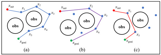
Figure 4.
Illustration of Dijkstra pruning. (a) The initial path; (b) the path improved using the pruning strategy based on triangle inequality for the results in (a); (c) the path improved using the Dijkstra pruning strategy for the results in (a), where the paths are marked in blue, purple, and red, respectively.
First, an adjacency matrix Value is used to record the distance between each state and the other states in the path. If there are obstacles blocking the connection between two states, the distance is set to infinity (line 1 in Algorithm 6). Then, three arrays, Visit, Path, and Dis, are set. Visit is used to record the visibility of each state. Path is used to record the predecessor node of each state. Dis is used to record the distance value from the initial state to each other state (line 1 in Algorithm 7). In each round, the minimum value is selected from Dis, and the corresponding state i in Visit is set to true (line 3–4 in Algorithm 7). Then, the relaxation operation is performed, such that:
If the distance from the initial state to state j can be improved by state i, state i is set as the predecessor node of state j (line 6–9 in Algorithm 7). The above operations are repeated until all states in Visit are visited. Finally, the shortest path is traced from the target state to the initial state via the array Path (line 12 in Algorithm 7).
| Algorithm 7. Dijkstra Pruning |
| Input: ηinit,Value Output: an optimized path η* 1: Visit.init, Path.init, Dis.init 2: for k = 1 to n − 1 do 3: i ← min(Dis) 4: Visit[i] ← True 5: for j = 1 to n do 6: if Dis[j] > Dis[i] + Value(i,j) then 7: Dis[j] ← Dis[i] + Value(i,j) 8: Path[j] ← i 9: end 10: end 11: end 12: η* ← Path |
An example of a utilization of the Dijkstra pruning strategy is shown in Figure 4. Let obstacles be denoted by obs. As shown in Figure 4a, the initial path is as follows: xinit–x1–x2–x3–x4–x5–xgoal. As shown in Figure 4b, starting from the initial state, three waypoints xinit, x1, and x2 are chosen in order. Note that the edge {xinit, x2} is free of collisions and the distance is shorter than the original route from xinit to x2. Therefore, the state x1 is considered to be a redundant node and the original route is replaced by the edge {xinit, x2}. Then, consider the relationship between the three waypoints xinit, x2, and x3, where the edge {xinit, x3} is not free of collisions. Therefore, the state xinit is traversed; starting from the next state x2, the same operation is executed until the target state is traversed. Finally, the path is determined to be as follows: xinit–x2–x3–x4–xgoal. As shown in Figure 4c, in the first round, Visit[x1] is set to true, because the distance between x1 and the initial state is the shortest. There is a collision between xinit and x5, where the value of Dis[x5] is infinity. Note that the route from xinit to x5 can be improved by x1 via the relaxation operation; therefore, the predecessor node of x5 is set to x1. Then, taking the corresponding waypoint, the minimum value in Dis, the relaxation operations are repeated until the target state is traversed. Finally, the path is determined to be as follows: xinit–x1–x5–xgoal.
3.2.2. Interpolation
The path optimization method based on the Dijkstra pruning strategy can find the shortest path given the current results. However, the problem remains that overly small angles remain in the path; these are called sharp nodes. A path with large turning angles can affect the stability of the motion planning; meanwhile, a path with gentle turning angles can better meet the requirements of practical applications. Therefore, it is necessary to remove sharp nodes. To solve this problem, the interpolation optimization method is utilized. In simple terms, two states are inserted into the path instead of the original corner node.
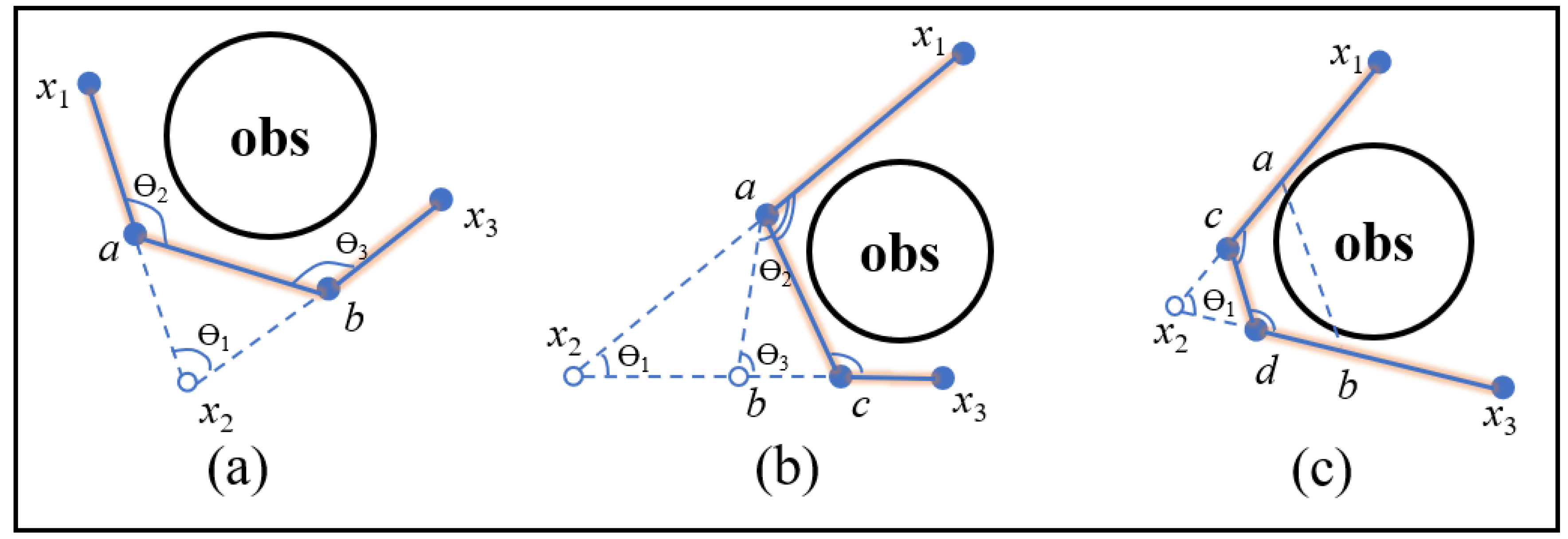
Specifically, if the angle Ɵ1 between the two adjacent vectors {x1, x2} and {x2, x3} is smaller than the threshold, then the middle nodes a and b of the two vectors {x1, x2} and {x2, x3} are calculated (line 2–4 in Algorithm 8). If there is no collision between the vector {a, b}, and the angle Ɵ2 between {x1, a} and {a, b} and the angle Ɵ3 between {b, x3} and {a, b} are greater than the threshold, then the two states, a and b, are added into the path instead of the original corner node x2 (line 5–8 in Algorithm 8). As shown in Figure 5a, two states, a and b, are inserted into the path instead of the original corner node x2. The modified path is as follows: x1–a–b–x3. If the angle Ɵ2 or Ɵ3 is still smaller than the threshold, the corner node with the larger angle and the middle node of the vector with the smaller angle are calculated; if this connection between the two states satisfies the conditions for insertion into the path, these two states are inserted into the path instead of the original corner node (line 9–14 in Algorithm 8). As shown in Figure 5b, the angle Ɵ3 is still smaller than the threshold after the first interpolation operation, then the two states, a and c, are inserted into the path instead of the original corner node x2. The modified path is as follows: x1–a–c–x3. If the vector {a, b} is not free of collisions after the first interpolation operation, the middle nodes of the vectors {a, x2} and {x2, b} are used to modify the path (line 15–17 in Algorithm 8). As shown in Figure 5c, the connection between a and b is not free of collisions after the first interpolation operation, then the two states, c and d, are inserted into the path instead of the original corner node x2. The modified path is as follows: x1–c–d–x3. This method not only eliminates sharp nodes in the path, but also shortens the path according to the principle of triangle inequality.
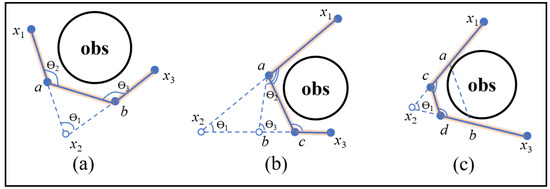
Figure 5.
Illustration of interpolation optimization. The blue dotted lines represent the cut and add operations. The modified path is marked with an orange outline. (a) An edge can be directly inserted into the path; (b) a sharp node still exists after inserting an edge; and (c) the inserted edge is not free of collisions.
| Algorithm 8. Interpolation |
| Input: Index, η* Output: an optimized path η* 1: for i = 1 to size(Index) do 2: Ɵ1 ← GetAngle(Index) 3: a ← GetMid(x1, x2) 4: b ← GetMid(x2, x3) 5: if CollisionFree(a, b, Map) then 6 if Ɵ2,Ɵ3 > threshold then 7: η*.delete() 8: η*.insert() 9: else 10: N ← GetNode(max(Ɵ2,Ɵ3)) 11: E ← GetEdge(min(Ɵ2,Ɵ3)) 12: M ← GetMid(E) 13: go to line 5 14: end 15: else 16: go to line 3 17: end 18: end |
4. Simulation and Analysis
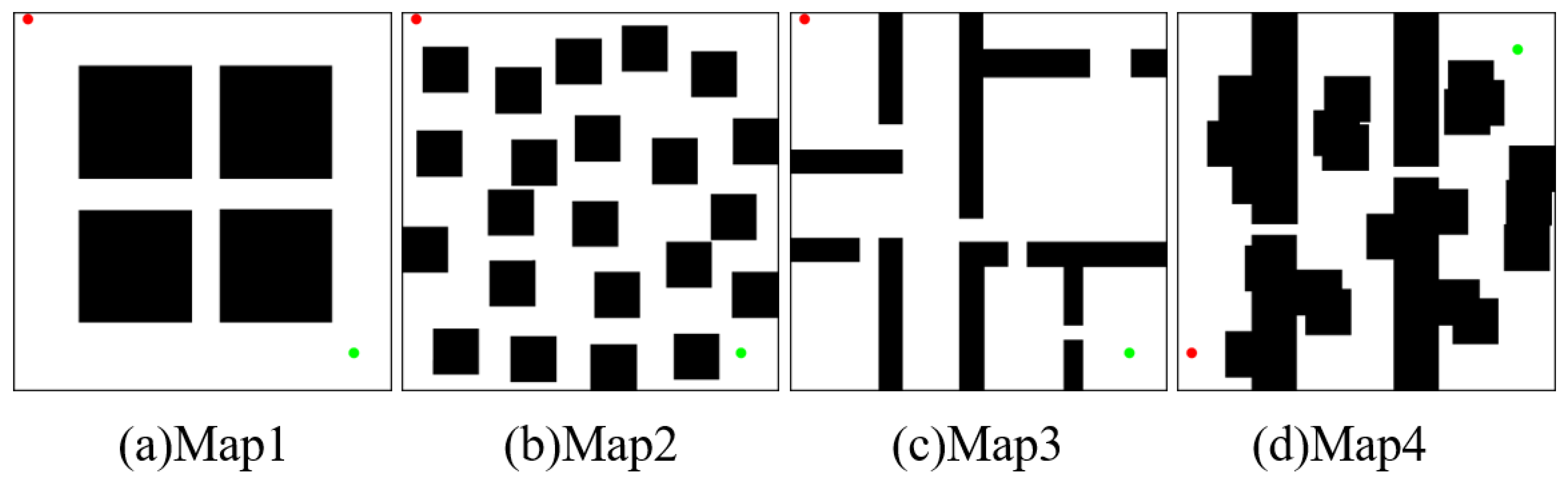
In this section, the results of two simulations, fast planning and path optimization, are presented, along with an analysis. As shown in Figure 6, four types of environments, denoted as Map1, Map2, Map3, and Map4, are utilized to simulate the path planning tasks. The resolutions of the four environments are all 500 × 500. In this planning tasks, area T is set to two-fifths of the entire area, while area M is set to seven-tenths of the entire area. The parameters for the experiments are shown in Table 1. If no path is found within the maximum number of iterations, the experiment is considered to be a failure. Each environment is run 50 times; it should be noted that only the data from the successful planning tests are used for the statistical analysis.
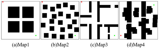
Figure 6.
Four types of planning task environments: (a) simple, (b) complex, (c) indoor, (d) narrow passages. The initial state and target state are marked by red and green points, respectively.

Table 1.
Parameters of the experiments.
The evaluation metrics are the computing cost, which consists of the running time and the average number of nodes, and the quality of the path. The corresponding standard deviation and planning success rate are also recorded. The running time reflects the time cost of different planners. The number of nodes represents the memory usage of different planners. The quality of the path is mainly reflected by the path length. The standard deviation and planning success rate indicate the stability of the planner.
All experiments were run on a computer based on an Intel i5-11300H 3.1 GHz CPU and 16 GB RAM, using MATLAB R2021a as the software platform.
4.1. Simulation of Fast Planning
In the fast planning experiment, we focused on the algorithm’s ability to quickly find paths in different scenarios. The running time and the number of nodes are important evaluation metrics, and the quality of the path is not considered. In order to verify the effectiveness of the proposed adjustable probability and sampling area strategies, the performance of the proposed APS-RRT planner is compared with that of the RRT and Bias-RRT algorithms. Statistical data based on the experiment results are presented in Table 2.
Table 2.
The statistical data for the simulation of fast planning.
Map1 is a simple environment for testing the performance of algorithms in a scenario with fewer obstacles. All three algorithms can achieve good results, but the APS-RRT planner makes considerable improvement in terms of the time cost and memory usage. Compared with the RRT and Bias-RRT algorithms, the APS-RRT planner reduces the running time by 57.1% and 40%, respectively. The APS-RRT planner also reduces the average number of nodes by 71.4% and 46.6%, respectively.
Map2 is a complex environment with multiple obstacles; it is used to test the performance of algorithms in the cluttered scenario. The Bias-RRT algorithm exhibit poor performance in Map2 and almost degenerates into the RRT algorithm, because the density of obstacles is high in this environment and the fixed goal bias probability makes the algorithm easily fall into a local minimum. However, the performance of the APS-RRT planner is not affected by this environment. The APS-RRT planner still maintains the efficient exploration capabilities, because it can adaptively adjust the goal bias probability and sampling area according to the growth status of the search tree, leading the planner to reach the target effectively. Compared with the RRT and Bias-RRT algorithms, in terms of the planning time, the APS-RRT planner reduces the average time cost by about 56.5%; the average number of nodes is reduced by 71.4% and 63%, respectively.
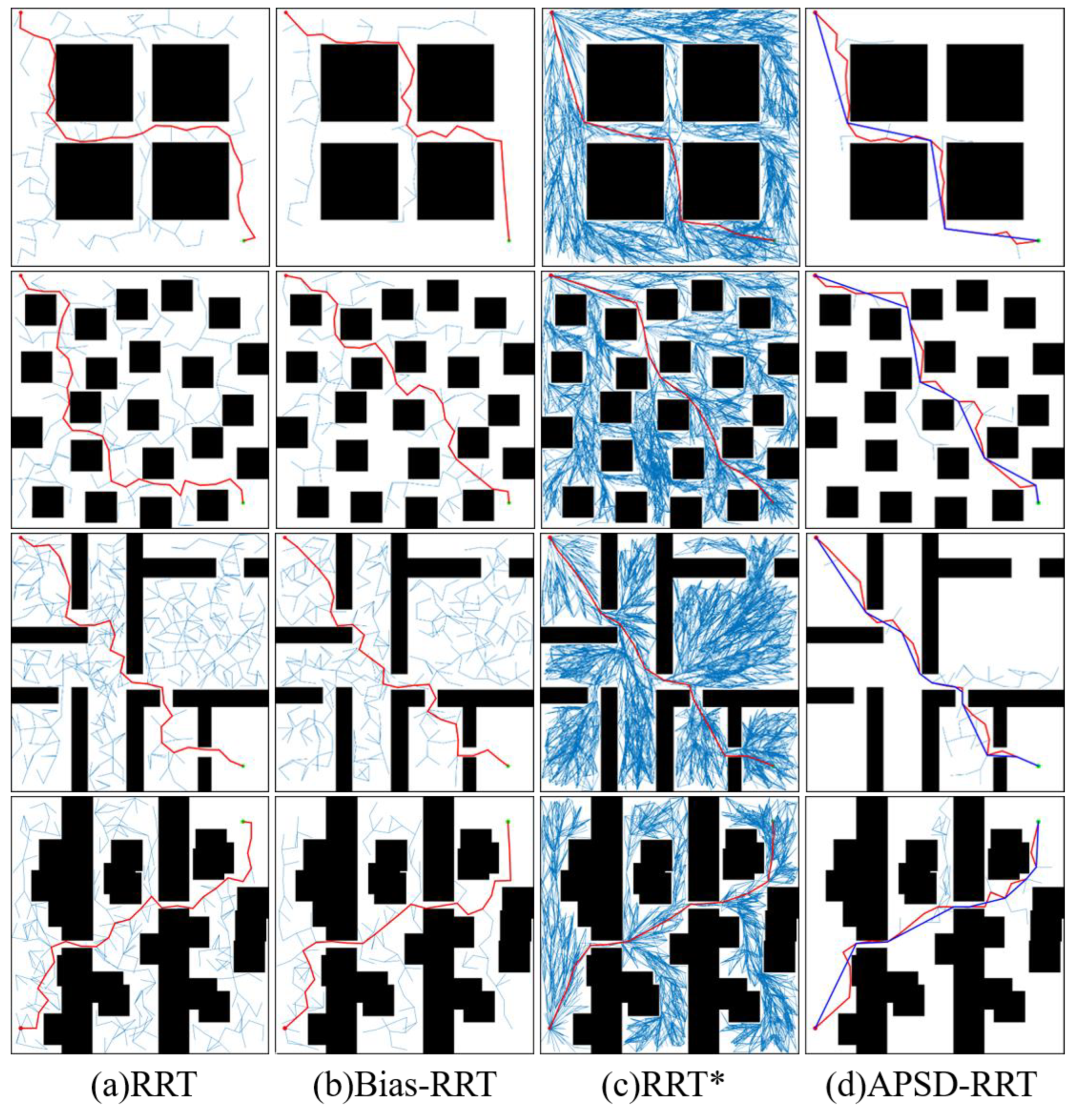
Map3 simulates an indoor scenario that contains many trap regions. The third row of Figure 7 shows that the nodes of the RRT and Bias-RRT algorithms fill almost the entire configuration space, but many nodes have no influence on the final path. The node redundancy of the two algorithms is a serious issue, because two of the planners have difficulty avoiding the trap regions, meaning that they consume a lot of computing resources. However, the APS-RRT planner can avoid unnecessary explorations in unimportant regions, where the solutions probably do not exist. Compared with the RRT and Bias-RRT algorithms, the APS-RRT planner has a significant improvement in terms of the running time, reducing 81.9% and 79.7%, respectively; the APS-RRT planner also reduces the average number of nodes by 82.6% and 76.1%, respectively. In Map3, the RRT algorithm has a success rate of 96%, the Bias-RRT algorithm has a success rate of 88%, and the APS-RRT planner maintains a success rate of 100%.
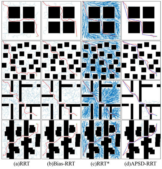
Figure 7.
From left to right in each row are the path planning results of the RRT, Bias-RRT, RRT* and APSD-RRT algorithms. The blue lines reflect the growth status of the search tree, and the red lines represent the generated path. The dark blue lines in (d) illustrate the optimized path.
Map4 represents the environment of narrow passages and contains many obstacles. The narrow passage environment poses a problem for sampling-based algorithms. This is because the probability of the samples falling within the passage is very low. The planning success rate of the RRT algorithm and the Bias-RRT algorithm drop significantly in Map4. In comparison, the APS-RRT planner maintains a high planning success rate, reflecting the performance of the proposed algorithm in the specific environment. Compared with the RRT and Bias-RRT algorithms, the APS-RRT planner reduces the average time cost by 50% and 46.9%, respectively, and the average number of nodes is reduced by 64% and 53.4%, respectively. In addition, the proposed APS-RRT has lower standard deviations. It is clear that the proposed algorithm can maintain stability and efficiency in different environments.
4.2. Simulation of Path Optimization
In this section, the proposed APSD-RRT algorithm is compared with the RRT and RRT* algorithms. The quality of the path is an important parameter in this experiment, which is measured by the initial path length (IPL) and the final path length (FPL). The corresponding time cost is also recorded, which is indicated by the initial time (IT) and the final time (FT). The statistical data based on the experiment results are presented in Table 3.
Table 3.
The statistical data for the simulation of path optimization.
The RRT algorithm aims to find a feasible solution, but it does not consider the path optimization. Once it finds the solution, the algorithm stops running. As shown in the first column of Figure 7, the paths generated by the RRT algorithm are tortuous, and do not meet the high-efficiency and energy-saving requirements of practical applications. The vectors obtained by the APS-RRT planner are relatively biased towards the target states; the quality of the path shows a slight improvement compared to the RRT algorithm, but there are many sharp and redundant nodes in the path. Compared with the RRT algorithm, the initial path lengths in the four environments are shortened by 9.4%, 6.3%, 8%, and 3.3%, respectively. Compared with the RRT* algorithm, the quality of the initial path generated in Map1 is slightly improved; in the other three environments, the initial path lengths are lengthened by 2.2%, 4.8% and 8%, respectively, but the time spent finding the initial path in the four environments is reduced by 67.9%, 67.7%, 90.2%, and 78.2%, respectively.
The RRT* algorithm achieved the final path with the best quality in this experiment, but the RRT* algorithm spends the most computing resources on the node optimization. It is clear that many nodes have no impact on the final result, especially in the environments with few obstacles, such as Map3, where there are many redundant nodes in the search tree. In comparison, the APSD-RRT algorithm is equipped with the post-processing methods to enhance the solution obtained by the APS-RRT planner. Benefiting from the planner’s speed when reaching a feasible solution, the APSD-RRT algorithm can generate a high-quality path within an acceptable time. The final path generated by the APSD-RRT algorithm is straight and smooth with few corners. It should be noted that the APSD-RRT algorithm shows an increase in the time cost of 26.4% on average and has the same memory usage than the APS-RRT planner, but it exhibits enhanced performance in terms of the quality of the path, shortening the path length by about 13% on average.
In the four different environments, the APSD-RRT algorithm shortens the final path length by about 19% on average compared with the RRT algorithm. In comparison with the RRT* algorithm, the APSD-RRT algorithm results in a higher-quality path in Map4; the APSD-RRT algorithm lengthens the path length by about 2.9% on average in the other three environments, but it has significant advantages in terms of the time cost and memory usage. Although the APSD-RRT algorithm exhibits a larger standard deviation in the performance of final path in Map2, the APSD-RRT method has significant advantages in terms of the balance between the computing cost and performance.
5. Conclusions
In this work, we propose a new sampling-based algorithm, APSD-RRT, which consists of two modules: an APS-RRT planner and an optimizer. Based on the growth status of the search tree, the planner can dynamically adjust the goal bias probability and the sampling area to improve the planning efficiency. The task of path optimization is separated into the optimizer, where the Dijkstra algorithm is used to obtain the shortest path and the interpolation strategy is implemented to smooth out sharp nodes. In terms of the balance between the computing cost and performance, the experiments demonstrate the effectiveness and efficiency of the APSD-RRT algorithm compared with the other algorithms.
APSD-RRT is an off-line algorithm. Only the path-planning problem based on the particle model in the static environment is considered in this work. In practical applications, it is necessary to consider non-holonomic constraints, where the direction of movement and turning angle of the mobile robot are restricted in real-world scenarios, and combine APSD-RRT with online algorithms, such as the dynamic window approach (DWA), to deal with uncertain situations.
The proposed path optimization strategies are post-processing methods, which have no impact on the performance of the planner. The final path quality depends on the initial path quality. Therefore, the performance in terms of path quality exhibits a certain degree of fluctuation. In future research, strategies such as Rewire in the RRT* algorithm may be equipped with the planner, which means that the quality of the initial path generated by the planner can be improved. However, it is certain that ensuring a better performance in terms of path quality will significantly increase the computing cost. Therefore, it is important to strike a balance between the computing cost and performance in meeting the specific requirements of different tasks. In addition, some advanced approaches ought to be considered for path optimization; inspired by [26], the evolutionary computation can be used to further improve the quality of the path and enhance the algorithm’s efficiency.
Author Contributions
Methodology, X.L.; simulation and analysis, X.L.; writing—review and editing, X.L. and Y.T. All authors have read and agreed to the published version of the manuscript.
Funding
This research received no external funding.
Institutional Review Board Statement
Not applicable.
Informed Consent Statement
Not applicable.
Data Availability Statement
Data are contained within the article.
Acknowledgments
The authors gratefully acknowledge the reviewers’ professional comments and the editors’ support of this work.
Conflicts of Interest
The authors declare no conflict of interest.
References
- Zafar, M.N.; Mohanta, J. Methodology for path planning and optimization of mobile robots: A review. Procedia Comput. Sci. 2018, 133, 141–152. [Google Scholar] [CrossRef]
- Sánchez-Ibáñez, J.R.; Pérez-del-Pulgar, C.J.; García-Cerezo, A. Path planning for autonomous mobile robots: A review. Sensors 2021, 21, 7898. [Google Scholar] [CrossRef]
- Gul, F.; Mir, I.; Abualigah, L.; Sumari, P.; Forestiero, A. A Consolidated Review of Path Planning and Optimization Techniques: Technical Perspectives and Future Directions. Electronics 2021, 10, 2250. [Google Scholar] [CrossRef]
- Hart, P.E.; Nilsson, N.J.; Raphael, B. A formal basis for the heuristic determination of minimum cost paths. IEEE Trans. Syst. Sci. Cybern. 1968, 4, 100–107. [Google Scholar] [CrossRef]
- Khatib, O. Real-time obstacle avoidance for manipulators and mobile robots. Int. J. Robot. Res. 1986, 5, 90–98. [Google Scholar] [CrossRef]
- Potvin, J.-Y. Genetic algorithms for the traveling salesman problem. Ann. Oper. Res. 1996, 63, 337–370. [Google Scholar] [CrossRef]
- Ismail, A.; Sheta, A.; Al-Weshah, M. A mobile robot path planning using genetic algorithm in static environment. J. Comput. Sci. 2008, 4, 341–344. [Google Scholar]
- Kavraki, L.E.; Svestka, P.; Latombe, J.-C.; Overmars, M.H. Probabilistic roadmaps for path planning in high-dimensional configuration spaces. IEEE Trans. Robot. Autom. 1996, 12, 566–580. [Google Scholar] [CrossRef]
- LaValle, S.M. Rapidly-Exploring Random Trees: A New Tool for Path Planning, TR 98-11; Department of Computer Science, Iowa State University: Ames, IA, USA, 1998. [Google Scholar]
- Karaman, S.; Frazzoli, E. Sampling-based algorithms for optimal motion planning. Int. J. Robot. Res. 2011, 30, 846–894. [Google Scholar] [CrossRef]
- Gammell, J.D.; Srinivasa, S.S.; Barfoot, T.D. Informed RRT: Optimal sampling-based path planning focused via direct sampling of an admissible ellipsoidal heuristic. In Proceedings of the 2014 IEEE/RSJ International Conference on Intelligent Robots and Systems, Chicago, IL, USA, 14–18 September 2014; pp. 2997–3004. [Google Scholar]
- Nasir, J.; Islam, F.; Malik, U.; Ayaz, Y.; Hasan, O.; Khan, M.; Muhammad, M.S. RRT*-SMART: A rapid convergence implementation of RRT. Int. J. Adv. Robot. Syst. 2013, 10, 299. [Google Scholar] [CrossRef]
- Wu, Z.; Meng, Z.; Zhao, W.; Wu, Z. Fast-RRT: A RRT-based optimal path finding method. Appl. Sci. 2021, 11, 11777. [Google Scholar] [CrossRef]
- Huang, C.; Zhao, Y.; Zhang, M.; Yang, H. APSO: An A*-PSO hybrid algorithm for mobile robot path planning. IEEE Access 2023, 11, 43238–43256. [Google Scholar] [CrossRef]
- Cao, X.; Zou, X.; Jia, C.; Chen, M.; Zeng, Z. RRT-based path planning for an intelligent litchi-picking manipulator. Comput. Electron. Agric. 2019, 156, 105–118. [Google Scholar] [CrossRef]
- Kuffner, J.J.; LaValle, S.M. RRT-connect: An efficient approach to single-query path planning. In Proceedings of the 2000 ICRA. Millennium Conference. IEEE International Conference on Robotics and Automation. Symposia Proceedings (Cat. No. 00CH37065), San Francisco, CA, USA, 24–28 April 2000; pp. 995–1001. [Google Scholar]
- Urmson, C.; Simmons, R. Approaches for heuristically biasing RRT growth. In Proceedings of the 2003 IEEE/RSJ International Conference on Intelligent Robots and Systems (IROS 2003) (Cat. No. 03CH37453), Las Vegas, NV, USA, 27–31 October 2003; pp. 1178–1183. [Google Scholar]
- Gan, Y.; Zhang, B.; Ke, C.; Zhu, X.; He, W.; Ihara, T. Research on robot motion planning based on RRT algorithm with nonholonomic constraints. Neural Process. Lett. 2021, 53, 3011–3029. [Google Scholar] [CrossRef]
- Chai, Q.; Wang, Y. RJ-RRT: Improved RRT for Path Planning in Narrow Passages. Appl. Sci. 2022, 12, 12033. [Google Scholar] [CrossRef]
- Huang, S. Path planning based on mixed algorithm of RRT and artificial potential field method. In Proceedings of the 2021 4th International Conference on Intelligent Robotics and Control Engineering (IRCE), Lanzhou, China, 18–20 September 2021; pp. 149–155. [Google Scholar]
- Wang, J.; Meng, M.Q.-H. Optimal path planning using generalized voronoi graph and multiple potential functions. IEEE Trans. Ind. Electron. 2020, 67, 10621–10630. [Google Scholar] [CrossRef]
- Chen, Y.; Cheng, C.; Zhang, Y.; Li, X.; Sun, L. A neural network-based navigation approach for autonomous mobile robot systems. Appl. Sci. 2022, 12, 7796. [Google Scholar] [CrossRef]
- Ichter, B.; Harrison, J.; Pavone, M. Learning sampling distributions for robot motion planning. In Proceedings of the 2018 IEEE International Conference on Robotics and Automation (ICRA), Brisbane, Australia, 21–25 May 2018; pp. 7087–7094. [Google Scholar]
- Li, Y.; Cui, R.; Li, Z.; Xu, D. Neural network approximation based near-optimal motion planning with kinodynamic constraints using RRT. IEEE Trans. Ind. Electron. 2018, 65, 8718–8729. [Google Scholar] [CrossRef]
- Wang, J.; Chi, W.; Li, C.; Wang, C.; Meng, M.Q.-H. Neural RRT*: Learning-based optimal path planning. IEEE Trans. Autom. Sci. Eng. 2020, 17, 1748–1758. [Google Scholar] [CrossRef]
- Liu, Z.; Yang, D.; Wang, Y.; Lu, M.; Li, R. EGNN: Graph structure learning based on evolutionary computation helps more in graph neural networks. Appl. Soft Comput. 2023, 135, 110040. [Google Scholar] [CrossRef]


Disclaimer/Publisher’s Note: The statements, opinions and data contained in all publications are solely those of the individual author(s) and contributor(s) and not of MDPI and/or the editor(s). MDPI and/or the editor(s) disclaim responsibility for any injury to people or property resulting from any ideas, methods, instructions or products referred to in the content. |
© 2023 by the authors. Licensee MDPI, Basel, Switzerland. This article is an open access article distributed under the terms and conditions of the Creative Commons Attribution (CC BY) license (https://creativecommons.org/licenses/by/4.0/).