Multiscale Feature-Based Infrared Ship Detection

Abstract

In this paper, based on the idea of “step-by-step accuracy”, a novel multiscale feature-based infrared ship-detection method (MSFISD) is proposed. The proposed method can achieve efficient and effective infrared ship detection in complex scenarios, which may provide assistance in applications such as night surveillance. First, candidate regions (CRs) are extracted from the whole image by extracting the sea–sky line and region of interest (ROI). The real sea–sky line is extracted based on the gradient features enhanced by large-scale gradient operators. The coarse segmentation results are obtained by the optimization method and are then refined by incorporating the edge features of the ship to reduce false alarms and obtain the CRs. Second, by analyzing the shape features of ships, the feature quantity is established, and the ships in CRs are finally accurately segmented. Experimental results demonstrate that compared with the other five methods, the proposed method has higher detection accuracy with a lower false-alarm rate and performs better in complex sea scenarios.

1. Introduction

Night vision imaging technology serves as a critical component in a wide range of contemporary optics-based applications, including night surveillance, assisted driving, and underwater detection. Its significance stems from its ability to enable effective visual perception in low-light environments, for example, in nighttime marine scenarios where the detection of ships is undertaken. The precise identification of ships in sea scenarios is of great significance for marine resource monitoring and coastguard enforcement, among other applications [1,2]. Infrared cameras, known for their advantages of long detection ranges and all-weather functionality, are widely utilized in various applications. However, the presence of buildings, reefs, islands, and sea clutter in complex sea surface scenarios, as well as limited resolution, poses significant challenges to the task of ship detection. Infrared image processing plays a paramount role in night vision imaging technology, enabling the extraction of valuable information from infrared images. It employs sophisticated algorithms and techniques to enhance image quality, detect objects, and facilitate object recognition [3,4,5].

In recent years, researchers have been exploring various methods for target detection in complex sea scenarios. The existing methods can be broadly divided into the following four categories: background-suppression based [6,7,8,9], active-contour based [10,11], feature-analysis based [12,13,14], and deep learning [15,16,17]. The background-suppression based method assumes that the grayscale distribution of the sea background is stable so that the modeling and estimation of the sea background can be achieved using different statistical models. After that, the foreground image is obtained by subtracting the background estimation from the original image. However, this method is not suitable for complex sea scenarios with a large amount of sea-clutter interference. By establishing an energy functional model, the active contour-based method firstly obtains the initial contour of the target and then continuously iterates until the contour converges with the real boundary. This method introduces the contour features of the ship in order to assist the segmentation while dealing with the complex sea surface background; disturbances such as islands, reefs, and clutter have similar contour characteristics to the target, which may lead to false alarms as well as the selection of the initial contour; the number of iterations will also affect the detection accuracy.

The key to the feature-analysis method is to select suitable features, not only to ensure that the features of the target itself are prominent and the difference between the target and the background is noticeable, but also to assess the difficulty and calculate the amount of feature extraction. In recent years, the deep-learning method has been widely studied with many detection algorithms proposed. Such methods face the problem of insufficient samples, and the number of network layers and parameter settings will directly affect the final detection accuracy and efficiency. In addition, a common issue in the existing methods is that it is hard to ensure the efficiency and real-time performance of target detection in global images; this remains an ongoing research challenge.

In view of the above problems, this paper proposes an infrared ship-detection method based on the idea of “step-by-step accuracy”, while considering various characteristics of the sea background and ships. First, CRs are extracted from the whole image by extracting the sea–sky line and ROI, and then, the final ship target extraction is accomplished by incorporating the shape features of the ship. The main purpose of this study is to improve the performance of infrared ship detection in complex scenarios, ensuring both effectiveness and high processing efficiency. The rest of this paper is organized as follows. In Section 2, the details of the proposed sea–sky line extraction and feature-based target extraction method are described. In Section 3, the experimental results, including the comparisons between the proposed method and the other five methods, are presented. Finally, the conclusion is presented in Section 4.

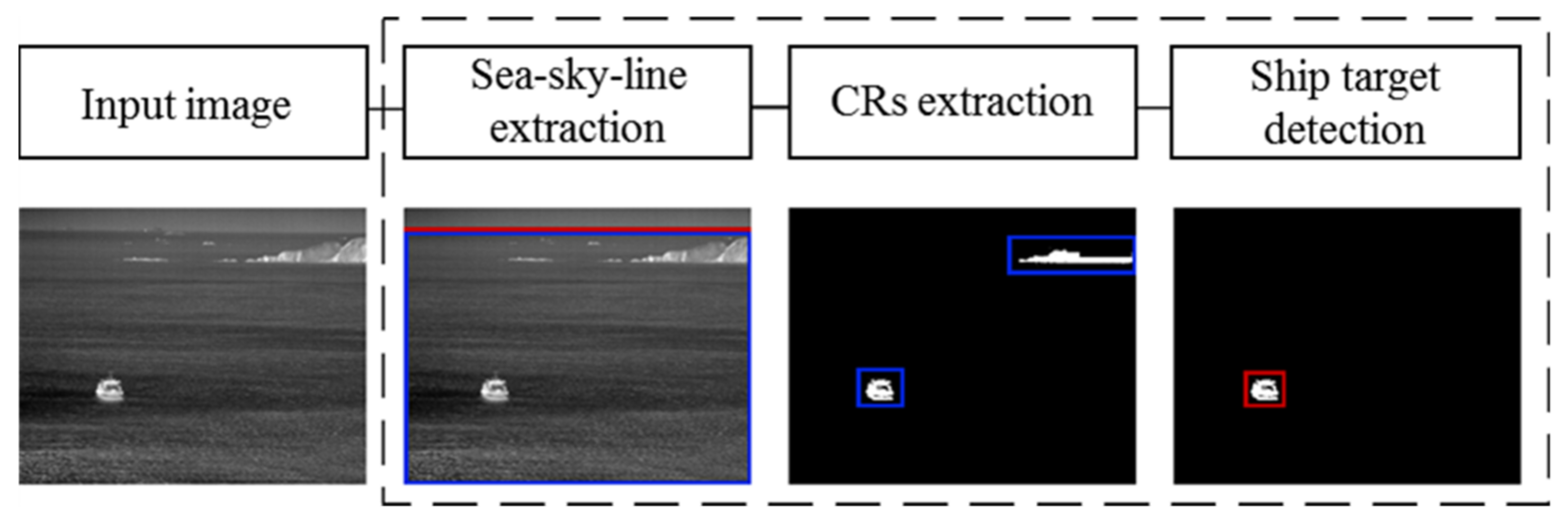
2. Materials and Methods

In this section, the detection framework of the proposed method is illustrated in Figure 1. We first extract the sea–sky line from the input image, then extract the CRs in the region below the sea–sky line. Finally, taking into account the distinct shape feature differences between ships, and interferences like islands and clutter, a set of feature-based thresholds is adopted to separate targets from CRs.

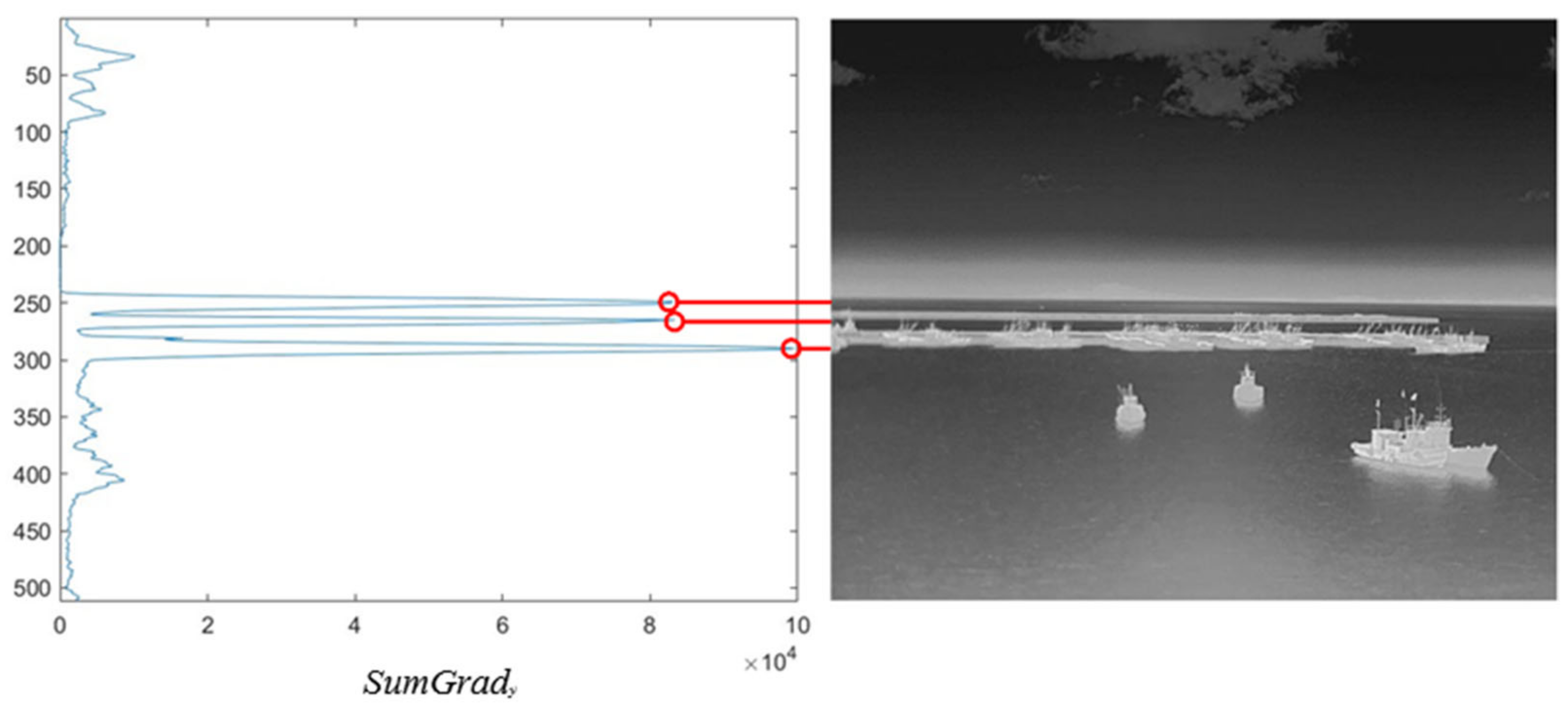
2.1. Multiscale Gradient Feature-Based Sea–Sky Line Extraction

In the images captured by forward-looking infrared cameras, ships are typically located below the sea–sky line. Therefore, the extraction of the sea–sky line in the image can exclude the interference from the sky and shore background and simultaneously reduce the area to be detected from the global image to the area below the sea–sky line. The sea surface exhibits a different radiation intensity and depth of field from the sky and shore background. As a result, the grayscale difference between the areas above and below the sea–sky line in the infrared image is distinct and can be characterized using gradient features. However, due to the low spatial resolution of infrared images, neighboring pixels exhibit a certain degree of correlation. Consequently, the sea–sky line may not be sufficiently prominent when calculating the gradient image using a small-scale gradient operator. In our method, interlacing in both rows and columns is used to increase the scale of gradient calculations, which can be described as Equation (1):

$$\left\{\begin{array}{l}gra{d}_x(i,j)=0.5\times \left|f(i-d_1,j)-f(i+d_1,j)+f(i-d_2,j)-f(i+d_2,j)\right|\\ gra{d}_y(i,j)=0.5\times \left|f(i,j-d_1)-f(i,j+d_1)+f(i,j-d_2)-f(i,j+d_2)\right|\end{array}\right.,$$

(1)

where grad_x(i, j), grad_y(i, j) represent the gradient value in the horizontal and vertical direction, respectively. f(i, j) is the intensity value of the pixel (i, j) in the input image.

As shown in Figure 2, the results of large-scale gradient map are presented, in which the values of d₁ and d₂ are set as 3 and 4, respectively. It is evident that the sea–sky lines in the vertical gradient images are significantly enhanced, appearing as generally long, approximately horizontal straight lines that traverse the entire image. Consequently, the vertical gradient images can be cumulated along the horizontal direction to highlight the position of the sea–sky line, which can be represented as Equation (2):

$$SumGra{d}_y(j)={\displaystyle \sum _{i=1}^{width}gra{d}_y}(i,j),$$

(2)

where width represents the number of the columns in the original image.

According to Equation (2), the results of SumGrad_y are presented in Figure 3, in which three local maximum values are highlighted. From the above results, it is observed that when there is more interference near the actual sea–sky line, the value of SumGrad at the location of the real sea–sky line may not be the highest but is still one of the three peaks. Therefore, SumGrad_y can serve as an effective basis for extracting the candidate positions of the sea–sky line. The extraction process for Pos(i), the candidate position of the sea–sky line, is shown in Figure 4.

The candidate positions derived from the previous processes may contain both cloud and clutter disturbances as well as the real sea–sky line, and so, further screening is necessary. As illustrated in Figure 2, cloud interference in the original image typically exists in the top area, while clutter interference occurs in the bottom area, with the real sea–sky line located in between. The grayscale changes more dramatically above the clouds and below the sea clutter, while it changes relatively gently above and below the sea–sky line. Therefore, a criterion for discriminating the sea–sky line can be proposed: the gradient values above the real sea–sky line are smaller, while the gradient values below it are larger. In contrast, the gradient values are larger above the cloud and smaller below it. Additionally, the gradient values are larger both above and below the sea clutter.

We select the areas above and below the candidate locations within the ω-rows range to calculate the gradient sum. Specifically, g₁ and g₂ denote the sum of the horizontal gradient, while g₃ and g₄ represent the sum of the vertical gradient, which can be written as Equations (3) and (4):

$$g_1={\displaystyle \sum _{d=1}^{\omega }{\displaystyle \sum _{i=1}^{width}gra{d}_h(i,j-d)}},g_2={\displaystyle \sum _{d=1}^{\omega }{\displaystyle \sum _{i=1}^{width}gra{d}_h(i,j+d)}},$$

(3)

$$g_3={\displaystyle \sum _{d=1}^{\omega }{\displaystyle \sum _{i=1}^{width}gra{d}_v(i,j-d)}},g_4={\displaystyle \sum _{d=1}^{\omega }{\displaystyle \sum _{i=1}^{width}gra{d}_v(i,j+d)}}$$

(4)

Then, two feature quantities for measuring the gradient features of the area near the candidate positions are defined as follows:

$$f_1=\frac{g_2}{g_1},f_2=\frac{g_4}{g_3},$$

(5)

where f₁ and f₂ represent the ratio of the horizontal gradient sum of the region below and above the candidate location and the ratio of the vertical gradient sum, respectively. Larger values of f₁ and f₂ indicate greater gradient differences between the regions above and below the candidate positions. According to the aforementioned criterion, the calculated f₁ and f₂ at the real sea–sky line position should be the largest of all candidate positions, which can be represented as Equation (6):

$$Skyline=find(f_1(Pos)+f_2(Pos))==\max (f_1(Pos)+f_2(Pos))$$

(6)

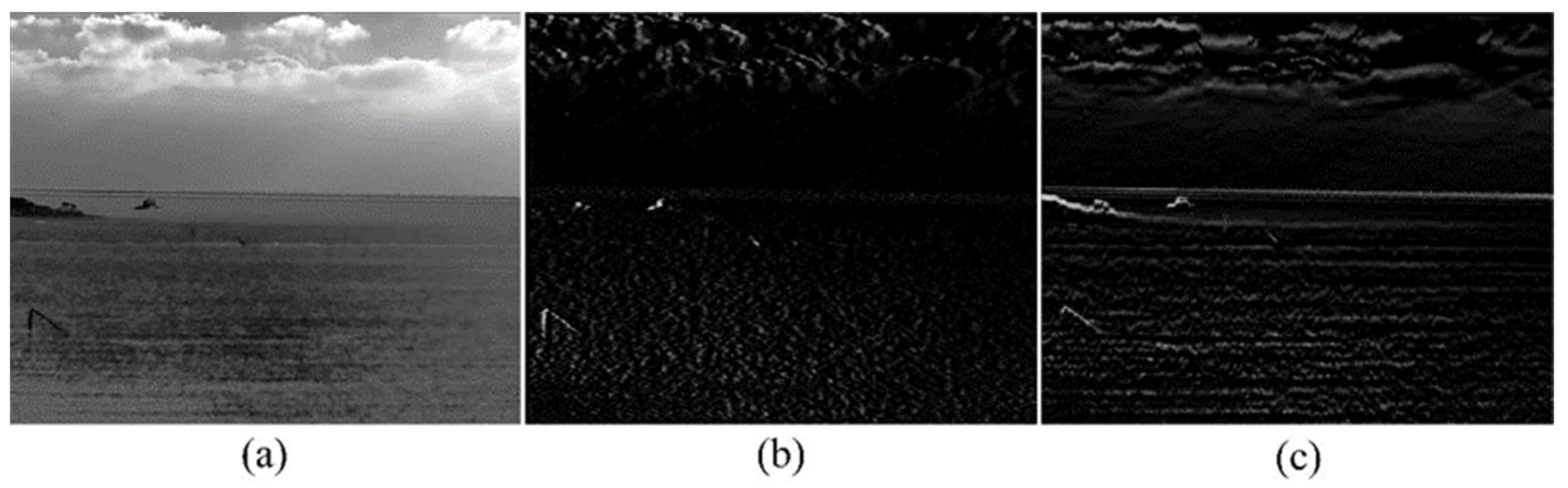
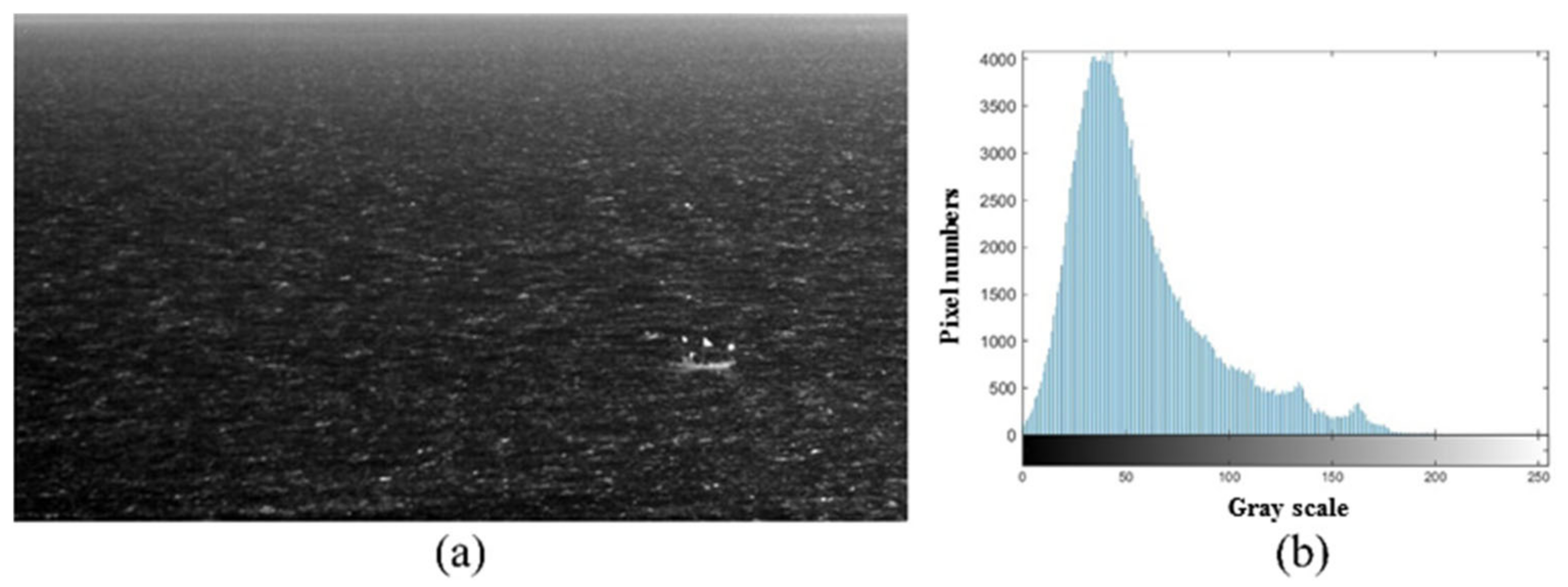
2.2. Candidate-Region Extraction Based on Grayscale and Edge Features

The images of the sea surface area excluding the sky and land are shown in Figure 5a, where the sea surface background occupies most of the pixels in the image and the ship target area is relatively small. There is a significant difference in grayscale distribution between the ship and the background. As is shown in Figure 5b, the histogram of the image of the sea surface area exhibits the distinct characteristics of a unimodal distribution, and the pixels of the sea surface background occupy most of the area.

The maximum entropy method [18] can calculate the segmentation threshold based on the intra-class grayscale probability of pixels, which can determine a reasonable segmentation threshold for the histogram with unimodal distribution and improve the segmentation effect when there exists significant contrast between the target and the background. However, this method involves multiple logarithmic operations when calculating the entropy values of the foreground and background, resulting in a time complexity of O(N²). In the case where the grayscale level of the image is 256, a total of 256² or 65,536 logarithmic operations are required. According to fractal theory, both entropy and correlation can be utilized to measure images; however, the time complexity of the latter is only O(N), meaning that when the grayscale of the image is 256, only 256 × 2 or 512 logarithmic operations are required. Therefore, correlation is employed here as a substitute replacing the entropy used to determine coarse segmentation [19].

Assuming that the sea surface area image has the number of rows H and the number of columns W and that the number of occurrences of the grayscale i in the histogram is h_i, the probability p_i of each grayscale can be calculated as:

$$p_i=h_i/(H·W)$$

(7)

Using the threshold T to split the image into background class B and foreground class O, the probability of foreground class and background class can be written as:

$${\omega }_o(T)={\displaystyle \sum _{i=T+1}^{256}{p}_i},$$

(8)

$${\omega }_b(T)={\displaystyle \sum _{i=1}^T{p}_i}=1-{\omega }_o$$

(9)

Supposing that X = {x₀, x₁, x₂,…} is a set of discrete random variables where p_i represents the probability of the variable x_i, the correlation of X can be defined as

$$C(X)=-\ln {\displaystyle \sum _{i\ge 0}{p}_i{}^2},$$

(10)

The sum of the correlations of the foreground and background after the segmentation, and the optimal segmentation threshold selection criterion, can be written as:

$$C(T)=-\ln {{\displaystyle \sum _{i=1}^T(\frac{p_i}{{\omega }_b(T)})}}^2-\ln {\displaystyle \sum _{T+1}^{256}{(\frac{p_i}{{\omega }_o(T)})}^2},$$

(11)

$$T=\arg \underset{1\le T\le 256}{\max }\{C(T)\}$$

(12)

Therefore, a coarsely segmented image can be obtained by using the following Equation (13):

$$B{W}_{MC}(i,j)=\left\{\begin{array}{l}1,I(i,j)>T\\ 0,otherwise\end{array}\right.$$

(13)

Since the coarse segmentation based on Equations (11)–(13) only takes grayscale features into consideration and ignores spatial information, it may result in the presence of significant clutter and isolated noise in the segmented image, as shown in Figure 6b. Taking into account the fact that ships in sea surface scenarios are generally closed connected regions with discernible edge contours, edge features can be adopted to further improve segmentation results. Here, we choose the Robert operator (Equation (14)), which allows us to calculate the cross gradient and extract the edge profile in the sea surface image; the edge feature image is calculated according to the following Equation (15):

$$Rober{t}_{{45}^{°}}=\left(\begin{array}{cc}0& -1\\ 1& 0\end{array}\right),Rober{t}_{{135}^{°}}=\left(\begin{array}{cc}-1& 0\\ 0& 1\end{array}\right),$$

(14)

$$I_{Edge}(i,j)=\left|f(i,j+1)-f(i+1,j)\right|+\left|f(i+1,j+1)-f(i,j)\right|$$

(15)

In order to remove false edges, the image I_Edge needs to be segmented using a threshold, which is calculated by using Equation (16):

$$T_e=\rho \cdot (Mean(I_{Edge})+Std(I_{Edge})),$$

(16)

where Mean and Std represent the mean value and standard deviation, respectively. The mean value is used as the basis of the threshold, while the standard deviation is able to characterize the number of edges present in the image, and finally, a control parameter ρ is employed to achieve adaptive segmentation. The final binary edge feature image can be calculated as:

$$B{W}_{Edge}=\left\{\begin{array}{l}1,I_{Edge}(i,j)>T_e\\ 0,otherwise\end{array}\right.$$

(17)

On the basis of the above results, we define here edge intensity E_n as a feature quantity to measure the edge features in the local area: the window of r × r size is moved in steps of r/2 across the binary edge feature map BW_Edge, from the top left to the bottom right, and the original image can be decomposed into image patches. Then, the number of non-zero pixels in each image block is counted as the edge intensity E_n according to Equation (19):

$$B{W}_{Edge}=[B{W}_1,B{W}_2,\cdot \cdot \cdot ,B{W}_n\cdot \cdot \cdot ,B{W}_N],$$

(18)

$$E_n=\#\{(i,j)\in B{W}_n\left|B{W}_{Edge}(i,j)=1\right.\},$$

(19)

where BW_n is the nth local image patch and #{} represents a counting operation.

Compared with the isolated noise points and residual sea surface clutter, ships tend to exhibit distinct edge contour characteristics, that is, they have large values of E_n. Therefore, the value of the edge intensity can be used to determine whether there is a candidate target in the local image patch:

$$B{W}_n=\left\{\begin{array}{l}1,E_n>\xi \\ 0,otherwise\end{array}\right.$$

(20)

After judging the edge intensity of all local image patches, those marked as 1 are clustered and remapped into the image matrix to obtain ROI images:

$$I_{ROI}(i,j)=\left\{\begin{array}{l}1,\forall (i,j)\in (B{W}_n=1)\\ 0,otherwise\end{array}\right.$$

(21)

The ROI images and the coarse-segmented images (based on Equation (13)) are then logically combined to obtain the final CRs:

$$I_{CR}(i,j)=B{W}_{MC}\&\&I_{ROI}(i,j)$$

(22)

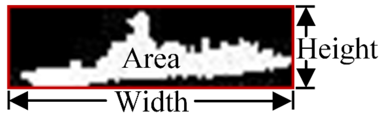
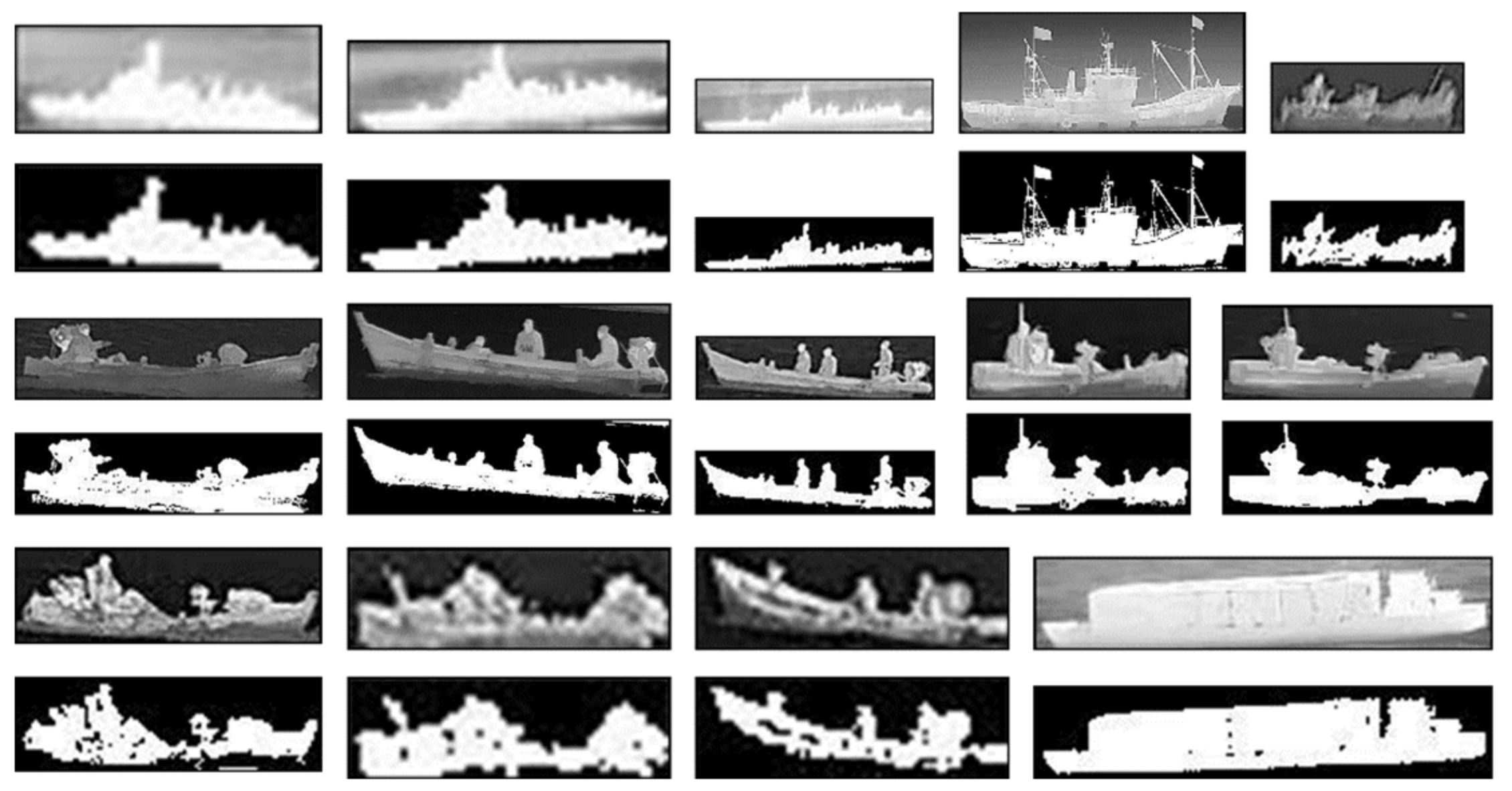
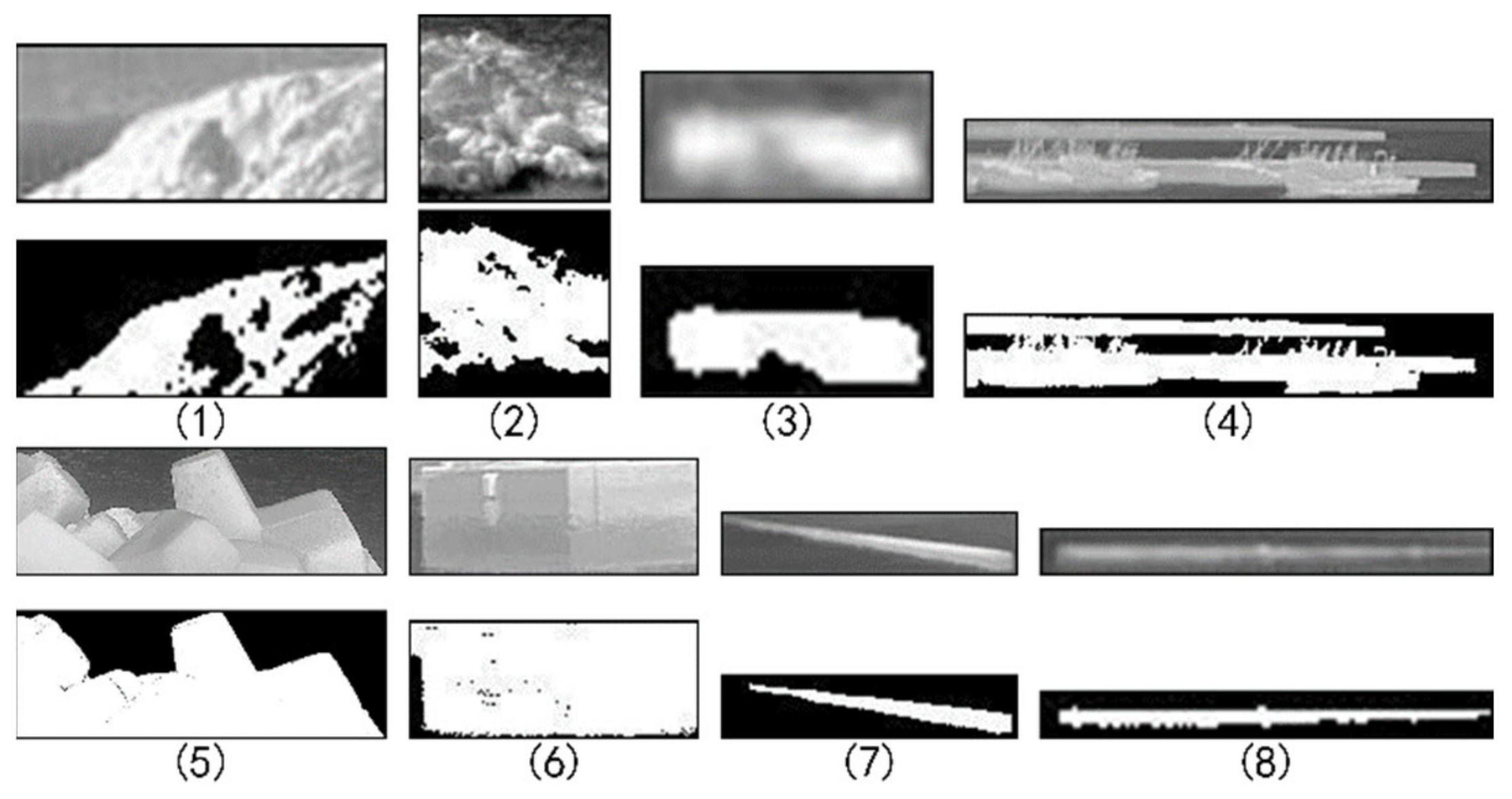
2.3. Ship Targets Extraction Based on Shape Features

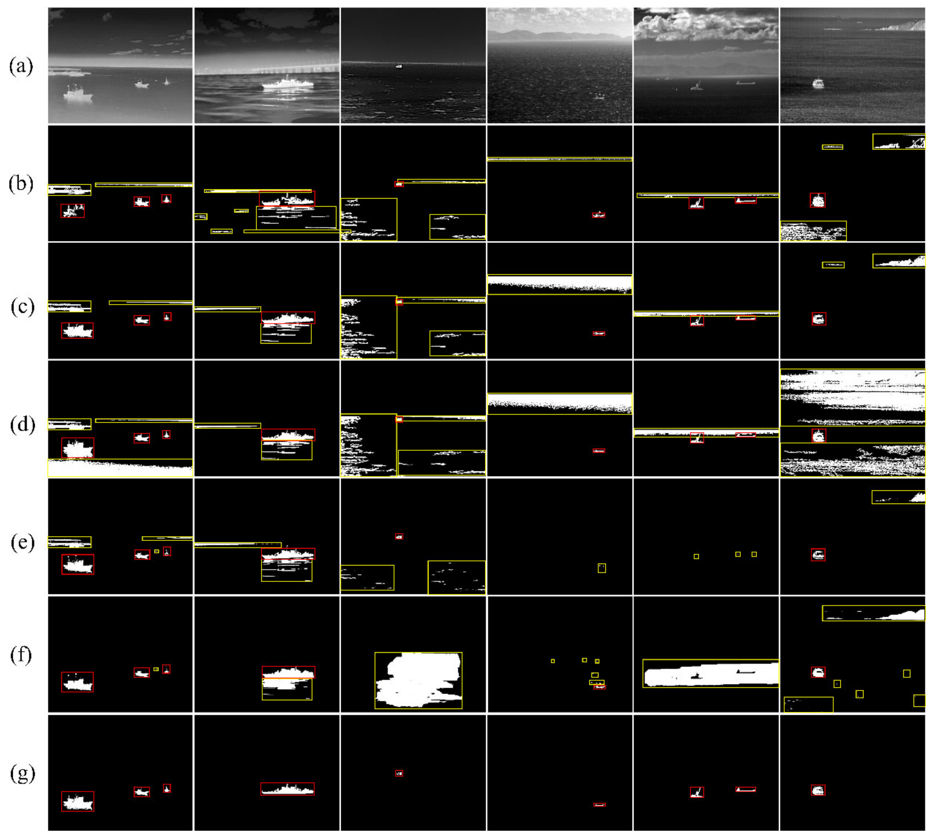
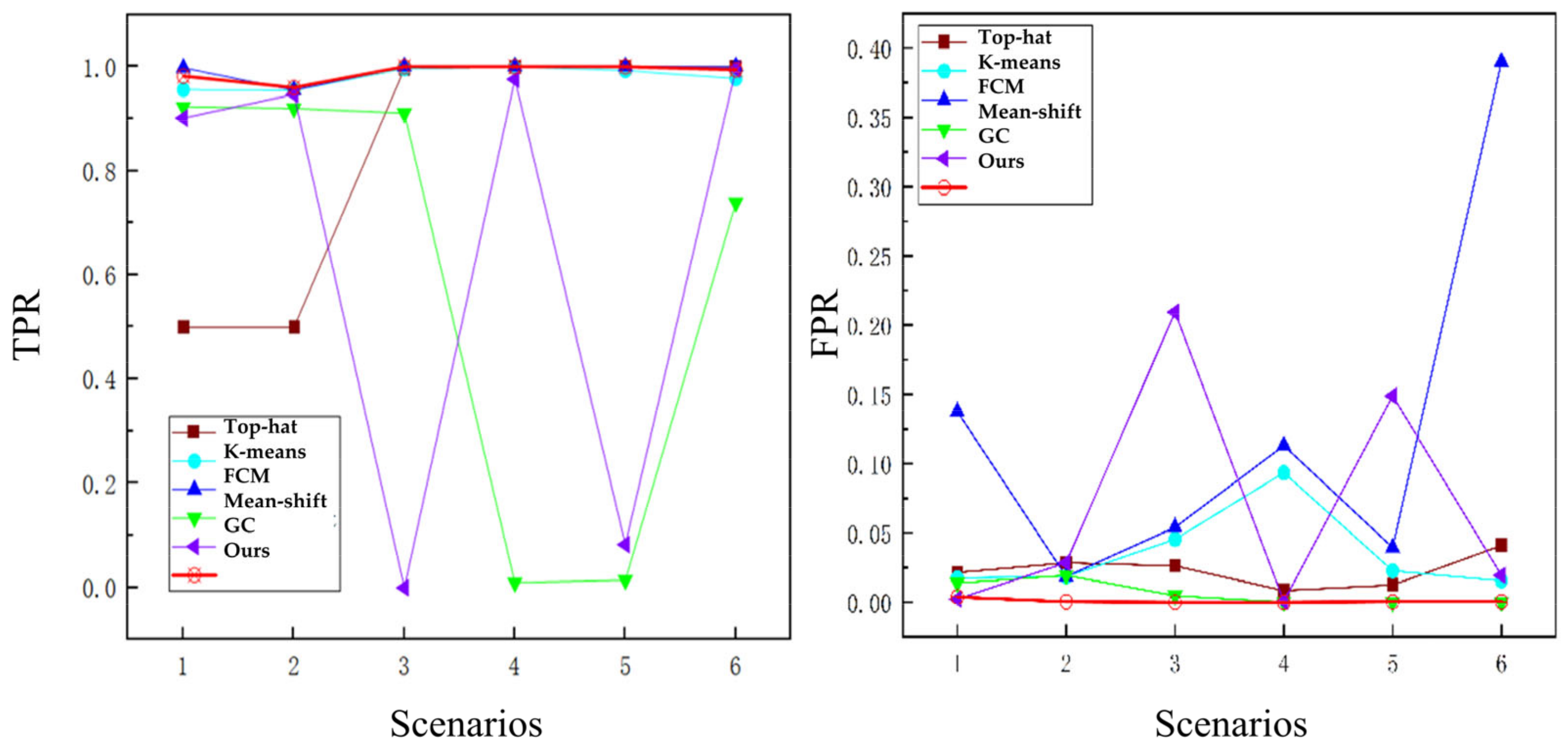
In complex sea surface scenarios, apart from the ships, there might still exist a series of interferences in the extracted CRs, such as sea clutter, islands, reefs, and buildings along the shore, which can lead to false alarms. Therefore, it is necessary to distinguish all the CRs to accurately detect the real ship targets. Shape is one of the most important features of infrared targets, and ship targets tend to have more regular shapes in the sea surface scene. In contrast, interferences are more random and have varied shape characteristics. Here, we choose aspect ratio F_WH, compactness F_z, duty cycle F_D, and signal-to-clutter ratio F_C as the shape characteristics to measure the ships:

$$F_{WH}(i)=\frac{Width}{Height},F_Z(i)=\frac{{(Perimeter)}^2}{Area},F_D(i)=\frac{Area}{Rectangle},F_C(i)=\frac{{\mu }_T-{\mu }_B}{{\sigma }_B},$$

(23)

where Width and Height are the size, Perimeter and Area represent the circumference and the area of the CRs, Rectangle is the area of the bounded rectangle of the CRs, and μ_T and μ_B are the average gray value of the target area and background area with σ_B as the standard deviation, respectively, as shown in Figure 7.

The key to identifying ships using shape features is to establish an appropriate range of parameters that can accurately distinguish between targets and other disturbances on the sea surface. In order to ensure the effectiveness and stability of the parameter range, we utilize here the infrared offshore ship dataset provided by IRay Technology Co., Ltd. (Yantai, Shandong, China), which contains more than 1000 infrared images of ships. After screening and deduplication, a total of 300 ships in five categories—warships, cruise ships, cargo ships, fishing boats, and yachts—are selected as positive samples to calculate and count the feature quantities according to Equation (23). Some of the ship slices and their binary images are shown in Figure 8. The statistical results are shown in

Table 1. The statistical results of the shape features of the 300 ships.

Feature Quantity	Minimum	Mean	Maximum
$F_{WH}$	1.0402	4.2566	13.4242
$F_Z$	17.6075	65.4393	137.6387
$F_D$	0.3827	0.5514	0.8213
$F_C$	0.1035	0.2141	0.3948

.

It should be noted that the objects of this paper are tangible ships occupying a certain area, so CRs of less than 30 pixels will be excluded. After obtaining the statistical results, the constraint ranges of the feature quantities are set as follows:

$$F_{WH}\_L=1.0402F_{WH}\_H=13.4242,$$

(24)

$$F_Z\_L=17.6075F_Z\_H=137.6387,$$

(25)

$$F_D\_L=0.3827F_D\_H=0.8213,$$

(26)

$$F_C\_L=0.1035F_C\_H=0.3948$$

(27)

The corresponding discriminant method is shown in Figure 9:

In order to prove the effectiveness of the constraint range and discriminant method proposed, the disturbing substances in different sea surface scenarios are selected as negative samples, and their feature quantities are calculated and then evaluated according to the above method. The selected negative samples are shown in Figure 10, with the calculated feature quantities displayed in

Table 2. The feature quantities of the negative samples and judgment results.

Num.	FWH	FZ	FD	FC	Judgment Results
(1)	2.3889	36.4018	0.8717	0.2739	FD > FD_H, Non-target
(2)	0.9667	40.8619	0.8291	0.3412	FD > FD_H, Non-target
(3)	3.3333	23.3506	0.8979	0.2714	FD > FD_H, Non-target
(4)	6.5526	226.3472	0.5453	0.2561	FZ > FZ_H, Non-target
(5)	2.9632	185.8927	0.5574	0.2166	FZ > FZ_H, Non-target
(6)	2.5098	21.7075	0.9448	0.3397	FD > FD_H, Non-target
(7)	5.0800	87.2140	0.2626	0.1184	FD < FD_L, Non-target
(8)	19.6000	145.2449	0.5775	0.0737	FWH > FWH_H, Non-target

. It is observed that one or more of the feature quantities of the negative samples do not fall within the constraint range and are therefore determined to be non-targeted. This empirical analysis confirms that the proposed method based on constraint ranges and discriminant features can effectively distinguish between real ship targets and other interferences present on the sea surface.

3. Results

Here, different sea surface scene images were selected for testing, in which scenes 1–2 were collected using medium-wave thermal imagers without coolers, and scenes 3–6 were collected using medium-wave refrigerated thermal imagers, with the resolutions set as 640 pixels × 512 pixels. All the experiments were carried out in MATLAB R2018b, on a computer with Intel(R) Core(TM) i5 CPU and 8 GB memory. To provide a comprehensive assessment, we compared our method with five other algorithms: top-hat, K-means clustering, fuzzy C-means clustering (FCM), mean shift, and grab-cut (GC). The results of all the tested algorithms, including our method and the five comparison algorithms, are presented in Figure 11. These results allow for a visual comparison and analysis of the segmentation outcomes obtained by each algorithm on the tested sea surface scene images.

Figure 11a shows the original infrared image in different scenarios. Interferences such as buildings, reefs, and sea clutter in the sea surface area can disturb the detection of the real ship targets. It can be seen from Figure 11b that the top-hat can detect all the real ship targets in different scenarios, while there still exist a large number of false alarms. Moreover, depending on the selected structural elements’ size, some detected ship targets may appear incomplete. The K-means, a cluster algorithm with strong spatial correlation, adopting the Euclidean distance between gray values, achieves relatively complete segmentation results, while it generates numerous false alarms in complex areas. Unlike the K-means, the FCM is a fuzzy clustering algorithm, into which membership is introduced to classify different pixels. As is shown in Figure 11d, the FCM is highly sensitive to noise. While targets in relatively flat areas can be separated from the background, this method generates the highest number of false alarms among all the methods. By utilizing merge operations based on the grayscale features of the local area, the mean-shift can reduce false alarms caused by small-scale interferences. However, if the grayscale difference between the ship and the background is small, this method is prone to missed detections and sometimes fails to detect the real targets. The GC, combining the ideas of K-means clustering and background modeling, can perform clustering and determine whether pixels are the target or not by establishing background and foreground models using the Gaussian mixture model. However, manual selection of the candidate area is required, as all the unselected area will be considered as background, and the final segmentation result is dependent on the box selection in scenarios where only parts of the sea surface area, including all the ships, are manually selected. As shown in Figure 11f, the ships in the first scenario were extracted completely, while in other scenarios, some targets were absorbed by the background. Among the above comparison methods, iterative calculation is inevitable in all the methods except for the top-hat, and as a result, the calculation amount is huge, and real-time processing cannot be achieved. Nevertheless, our method can detect and segment all the targets and remove false alarms in CRs with single determination. Figure 11g gives the results of our method, and it can be seen that the segmented ship targets exhibit complete shape and contour, showing clear advantages over other methods evaluated.

4. Discussion

In order to quantitatively evaluate the performance of each algorithm, two evaluation indicators, true positive rate (TPR) and false positive rate (FPR), are selected for comparison. TPR and FPR are calculated as follows:

$$\mathrm{TPR}=\frac{\mathrm{TP}}{\mathrm{TP}+\mathrm{FN}},\mathrm{FPR}=\frac{\mathrm{FP}}{\mathrm{FP}+\mathrm{TN},}$$

(28)

where TP and FN represent the number of the detected and undetected pixels of the real targets, with FP, the number of misjudged pixels as the target, and TN, the number of correctly judged pixels as the target.

In order to quantitatively evaluate the detection performance of each algorithm, a reference image containing the ground truth labels for real targets and background pixels is manually annotated. The test results of each method are compared with the reference image and calculated by Equation (28).

Table 3. The comparison results of all the algorithms. The bold represent the best results in different scenarios.

		Top-Hat	K-Means	FCM	Mean-Shift	GC	Our Method
S1	TPR	0.4992	0.9558	0.9973	0.9225	0.9010	0.9817
	FPR	0.0215	0.0177	0.1376	0.0138	0.0022	0.0038
S2	TPR	0.4992	0.9547	0.9547	0.9196	0.9466	0.9598
	FPR	0.0285	0.0186	0.0186	0.0194	0.0286	0.0004
S3	TPR	0.9960	0.9960	1.0000	0.9101	0.0000	1.0000
	FPR	0.0263	0.0454	0.0541	0.0047	0.20947	0.0000
S4	TPR	1.0000	1.0000	1.0000	0.0097	0.97573	1.0000
	FPR	0.0084	0.0935	0.1132	0.0001	0.0006	0.0000
S5	TPR	1.0000	0.9922	1.0000	0.0146	0.0828	1.0000
	FPR	0.0124	0.0227	0.0394	0.0000	0.1490	0.0003
S6	TPR	1.0000	0.9772	1.0000	0.7392	0.9952	0.9937
	FPR	0.0410	0.0155	0.3902	0.0060	0.0195	0.0003

presents the comparison results. The definition of the TPR and FPR indicates that the larger the calculated TPR value and the smaller the FPR value, the better the performance of the detection algorithm. That is, it has a low false-alarm rate while having high detection accuracy. The comparison results in Table 3 and Figure 12 demonstrate that the top-hat performs well in scenarios 4–6, with a relatively flat background, but shows a higher false-alarm rate in the more complex scenarios 1–3. The calculation results of TPR indexes obtained by K-means and FCM are similar, both being close to 1, indicating that both methods can completely extract targets, but there still exists the problem of a high false-alarm rate, especially for the KCM. The mean-shift has a small FPR across all the selected scenarios, but its TPR indicator is also small, especially in scenarios 4 and 5, where targets are missed, in which the TPR values are close to 0. The GC algorithm shows unstable TPR and FPR values; although the detection rate is high in some scenarios, some targets are still missed in other scenarios, and the TPR value is close to or equal to 0, which proves that there exists instability because manual selection is inevitable for the GC. In contrast, the proposed method consistently achieves both ideal TPR and FPR across different scenarios, indicating that it can accurately detect ships in both simple and complex sea surface scenarios, unaffected by various disturbances. In summary, our method has significant advantages over the other five methods in terms of both detection accuracy and low false-alarm rate and can complete the task of accurate infrared detection of ships under a complex sea surface background. Moreover, the calculation of the selected feature quantities is simple; thus, it can achieve highly efficient detection.

5. Conclusions

In this paper, based on the idea of “step-by-step accuracy”, we propose a novel multiscale feature-based infrared ship-detection method (MSFISD). The proposed method can efficiently and effectively achieve infrared ship detection in complex scenarios, which may provide assistance in applications such as night surveillance or remote piloting. First, CRs are extracted from the whole image by extracting the sea–sky line and ROI and are refined by incorporating the edge features of the ship to reduce false alarms. Finally, by analyzing the shape features, the ship targets are finally accurately extracted. Experimental results demonstrate that compared with the other five methods, our method has a higher detection accuracy with a lower false-alarm rate and shows excellent detection performance. However, our method still has limitations. Firstly, in scenes with large-scale interferences, such as islands or bright and dark bands, it is a challenging task to accurately extract the sea clutter. In these scenarios, large areas of islands or reefs may obscure parts of the sea–sky line in images, resulting in ocean boundaries with potentially intricate shapes. Secondly, under certain lighting conditions in which the sea surface exhibits severe fluctuations, it becomes difficult to distinguish clutter, which resembles the grayscale and shape of ships. In future work, we will extend the method of sea–sky line extraction to a more universal marine area extraction and improve and innovate both the single-frame detection and multi-frame detection algorithms to achieve more accurate, stable, and robust infrared ship detection.

References

1. Prasad, D.; Rajan, D.; Rachmawati, L.; Rajabaly, E.; Quek, C. Video Processing from Electro-Optical Sensors for Object Detection and Tracking in a Maritime Environment: A Survey. IEEE Trans. Intell. Transp. Syst. 2016, 18, 1993–2016. [Google Scholar] [CrossRef]
2. Zhang, Z.; Shao, Y.; Tian, W.; Wei, Q.; Zhang, Y.; Zhang, Q. Application Potential of GF-4 Images for Dynamic Ship Monitoring. IEEE Geosci. Remote Sens. Lett. 2017, 14, 911–915. [Google Scholar] [CrossRef]
3. Bai, X.; Zhou, F.; Jin, T.; Xie, Y. Infrared Small Target Detection and Tracking under the Conditions of Dim Target Intensity and Clutter Background. Proc. SPIE 2007, 6786, 683–691. [Google Scholar] [CrossRef]
4. Wang, B.; Motai, Y.; Dong, L.; Xu, W. Detecting Infrared Maritime Targets Overwhelmed in Sun Glitters by Antijitter Spatiotemporal Saliency. IEEE Trans. Geosci. Remote Sens. 2019, 57, 5159–5173. [Google Scholar] [CrossRef]
5. Li, Y.; Li, Z.; Zhu, Y.; Li, B.; Xiong, W.; Huang, Y. Thermal Infrared Small Ship Detection in Sea Clutter Based on Morphological Reconstruction and Multi-Feature Analysis. Appl. Sci. 2019, 9, 3786. [Google Scholar] [CrossRef]
6. Gao, C.; Deyu, M.; Yang, Y.; Wang, Y.; Zhou, X.; Hauptman, A. Infrared Patch-Image Model for Small Target Detection in a Single Image. IEEE Trans. Image Process. 2013, 22, 4996–5009. [Google Scholar] [CrossRef] [PubMed]
7. Zhou, A.; Xie, W.; Pei, J. Background Modeling in the Fourier Domain for Maritime Infrared Target Detection. IEEE Trans. Circuits Syst. Video Technol. 2020, 30, 2634–2649. [Google Scholar] [CrossRef]
8. Zhou, A.; Xie, W.; Pei, J. Background Modeling Combined with Multiple Features in the Fourier Domain for Maritime Infrared Target Detection. IEEE Trans. Geosci. Remote Sens. 2021, 60, 1–15. [Google Scholar] [CrossRef]
9. Zhou, A.; Xie, W.; Pei, J. Maritime Infrared Target Detection Using a Dual-Mode Background Model. Remote Sens. 2023, 15, 2354. [Google Scholar] [CrossRef]
10. Fang, L.; Zhao, W.; Li, X.; Wang, X. A Convex Active Contour Model Driven by Local Entropy Energy with Applications to Infrared Ship Target Segmentation. Opt. Laser Technol. 2017, 96, 166–175. [Google Scholar] [CrossRef]
11. Fang, L.; Wang, X.; Wan, Y. Adaptable Active Contour Model with Applications to Infrared Ship Target Segmentation. J. Electron. Imaging 2016, 25, 041010. [Google Scholar] [CrossRef]
12. Liu, J.; Zhou, F.; Chen, X.; Bai, X.; Sun, C. Iterative Infrared Ship Target Segmentation Based on Multiple Features. Pattern Recognit. 2014, 47, 2839–2852. [Google Scholar] [CrossRef]
13. Liu, J.; Bai, X.; Sun, C.; Zhou, F.; Li, Y. Infrared Ship Target Segmentation through Integration of Multiple Feature Maps. Image Vis. Comput. 2016, 48, 14–25. [Google Scholar] [CrossRef]
14. Bai, X.; Chen, Z.; Zhang, Y.; Liu, J.; Lu, Y. Spatial Information Based FCM for Infrared Ship Target Segmentation. In Proceedings of the 2014 IEEE International Conference on Image Processing, ICIP 2014, Paris, France, 27–30 October 2014; Volume 46, pp. 5127–5131. [Google Scholar] [CrossRef]
15. Li, L.; Jiang, L.; Zhang, J.; Wang, S.; Chen, F. A Complete YOLO-Based Ship Detection Method for Thermal Infrared Remote Sensing Images under Complex Backgrounds. Remote Sens. 2022, 14, 1534. [Google Scholar] [CrossRef]
16. Han, Y.; Liao, J.; Lu, T.; Pu, T.; Peng, Z. KCPNet: Knowledge-Driven Context Perception Networks for Ship Detection in Infrared Imagery. IEEE Trans. Geosci. Remote Sens. 2022, 61, 1–19. [Google Scholar] [CrossRef]
17. Wu, T.; Li, B.; Luo, Y.; Wang, Y.; Xiao, C.; Liu, T.; Yang, J.; An, W.; Guo, Y. MTU-Net: Multi-Level TransUNet for Space-Based Infrared Tiny Ship Detection. IEEE Trans. Geosci. Remote Sens. 2023, 61, 1–15. [Google Scholar] [CrossRef]
18. Kapur, J.N.; Sahoo, P.; Wong, A.K.C. A New Method for Gray-Level Picture Thresholding Using the Entropy of the Histogram. Comput. Vis. Graph. Image Process. 1980, 29, 273–285. [Google Scholar] [CrossRef]
19. Yen, J.-C.; Chang, F.-J.; Chang, S. New Criterion for Automatic Multilevel Thresholding. Image Process. IEEE Trans. 1995, 4, 370–378. [Google Scholar] [CrossRef]
Figure 1. Framework of the proposed method. The red line shows the position of the extracted sea-sky-line, and the blue bounding box represent CRs where ship might exists.
Applsci 14 00246 g001
Figure 2. Large-scale gradient map. (a) Original image. (b) Horizontal gradient map. (c) Vertical gradient map.
Applsci 14 00246 g002
Figure 3. Result of SumGrady.
Applsci 14 00246 g003
Figure 4. Flowchart of the candidate positions for extraction of the sea–sky line.
Applsci 14 00246 g004
Figure 5. (a) Image and (b) histogram of the sea surface area.
Applsci 14 00246 g005
Figure 6. Process of extracting the CRs and the results. (a) Input preprocessed image. (b) Coarse-segmented image. (c) Binary edge feature map BWMC. (d) ROI map. (e) CRs map.
Applsci 14 00246 g006
Figure 7. Shape features of the ship.
Applsci 14 00246 g007
Figure 8. Positive samples and binary slices of different categories of ships.
Applsci 14 00246 g008
Figure 9. Flow chart of ship discrimination.
Applsci 14 00246 g009
Figure 10. Eight kinds of disturbing substances and binary slices.
Applsci 14 00246 g010
Figure 11. Processed results of different algorithms. (a) Original image. (b) Top-hat. (c) K-mean. (d) FCM. (e) Mean-shift. (f) GC. (g) Our method. The red boxes show the detected targets, and the yellow boxes represent the false alarms.
Applsci 14 00246 g011
Figure 12. TPR and FPR curves of different scenarios.
Applsci 14 00246 g012