Abstract
Reconfigurable intelligent surfaces (RISs) are acknowledged as one of the key technologies for the next-generation communication systems due to their low cost, high-energy efficiency, and the ability to intelligently control the wireless propagation environment. In this paper, we present a hybrid active–passive reconfigurable intelligent surface (HAPR) for cooperative transmission system, where HAPR can intelligently change its operating mode according to the channel environment, eliminating the “multiplicative fading” effect of traditional passive RIS (P-RIS) and higher power consumption of active RIS (A-RIS), and combining the advantages of both to effectively improve the system performance. First, we investigate the ideal reflection coefficient of RIS reflecting elements (REs) under the condition of a limited power budget. Using the compound Simpson formula, the closed-form approximation expression for the system outage probability (OP) has been derived. Finally, Monte Carlo simulation is used to confirm the accuracy of the expression. The simulation results demonstrate that HAPR has a better performance than both A-RIS and P-RIS, which can achieve a lower OP.
1. Introduction
With the approach of the beyond fifth generation mobile network (B5G)/6G era, the massive increase in wireless devices and smart terminals has made the traditional network environment increasingly complex, bringing serious communication problems [1]. Gratefully, the emergence of reconfigurable intelligent surfaces (RISs) presents an effective solution to these problems [2]. In recent years, RISs, which are considered one of the sixth generation wireless systems’ main technologies, have attracted wide attention in academia and industry because of their ability to change communication performance by using the implied randomness in the propagation environment [3]. RIS is an electromagnetic artificial surface made up of many near-passive reflecting elements (REs), which independently and efficiently adjusts the amplitude and phase of the incident signal through a controller. The controller can be programmed to reconfigure the electromagnetic signal, thus eliminating the need for elaborate decoding, encoding and radio frequency (RF) processing operations [4,5,6]. Moreover, passive RIS is reliant on tunable electronic circuits (such as varactors or PIN diodes) with low power consumption to change the phase, so the power consumption is almost zero [7]. As RIS is lightweight, it can be installed on a wide range of scattering surfaces, like buildings, roadside signage, windows, walls, etc. [8,9].
From the introduction of the RIS concept to the present day, a large number of studies and ideas have emerged regarding the performance analysis of RIS-assisted communication systems. In [10], the basic performance of RIS-assisted single-input single-output (SISO) communication systems under mixed Rayleigh and Rice fading channels were investigated, and expressions for the ergodic capacity (EC) and the outage probability (OP) were obtained using the central limit theorem (CLT) by assuming that the REs were sufficiently large. In parallel, the authors discovered that using RIS with N REs enabled the system achieve an effective signal-to-noise ratio (SNR) gain of . In [11], the authors proposed a wireless single-cell system with RIS assistance that demonstrated that passive RIS systems were less costly than conventional massive multiple-input multiple-output (MIMO) systems or multiple-antenna amplify-and-forward (AF) relaying with significantly improved energy efficiency, coverage, and achievable rates for wireless communication systems. The statistical channel state information (CSI)-based RIS-assisted MIMO system for secure transmission was studied in [12], confirming that there was an increase in the ergodic secrecy rate as the number of RIS REs increased. In addition, RIS can be integrated with various wireless technologies, such as millimeter wave (mmWave), non-orthogonal multiple access (NOMA), free space optics (FSO), visible light communication (VLC), unmanned aerial vehicle (UAV), and two-way communication, through which different communication objectives can be achieved [13,14,15,16,17,18].
While passive RIS has been proven to have many advantages that are unmatched by other technologies, passive RIS also has some shortcomings. For example, passive RIS-assisted systems may be limited by “multiplicative fading” effects. To be specific, the reflected signal needs to travel over a channel that is cascaded and made up of transmitter-RIS and RIS-receiver channels [19], and the path loss of this cascaded channel is a relationship in which the two channel losses are multiplied, rather than added. The “multiplicative fading” effect has the dire consequence that, in many cases with strong direct links, the expected capacity gain cannot be achieved using RIS [20]. If we want to increase the gain in the RIS-assisted system to a feasible level, the passive RIS necessitates a high number of REs, which results in an oversized RIS surface, which is not a viable solution in practical situations. Moreover, these passive REs are still limited by the power budget, which hinders the existing capability of passive RIS [21]. To mitigate the “multiplicative fading” effect, in [19], the notion of active RIS (A-RIS) is put forward, whereby it not only adjusts the phase of the incident signal, but also amplifies the incident signal to normal levels, as opposed to passive RIS. Additionally, active RIS still benefits from passive RIS’s advantages without the requirement for complicated and power-hungry RF chain components. When the total number of REs was low, the author of [7] observed that active RIS performed better than passive RIS when comparing the two under an identical power limitation. Ref. [20] revealed that in MIMO systems, comparatively speaking, active RIS could reach up to 67% sum-rate gain compared with passive RIS, while passive RIS was capable of only a meager 3% sum-rate gain, which was almost negligible. Ref. [22] studied the position of active RIS in wireless systems, and revealed that moving active RIS closer to the receiver was a good idea. The security performance of the active RIS-assisted wireless communication system was discussed in [23], where the authors found that the dependability of the signal transmission and the secrecy outage probability (SOP) could both be considerably increased by using active RIS. Notwithstanding the fact that active RIS performs better than passive RIS in particular, every active RE enhances the incident signal through a power amplifier, resulting in greater power consumption. Based on existing research, we are aware that improving the system’s performance will result from adding more REs to RIS, but when there are too many active RIS elements, it will lead to a high power consumption, which is contrary to our original intention of using RIS. In [24], the concept of an active RIS sub-connected architecture was proposed, where multiple REs control the phase shifts independently, but share the same power amplifier. Although this architecture is more energy efficient compared with controlling each RE with a single amplifier, each sub-connected architecture still requires 256 REs to achieve optimal energy efficiency (EE).
Recently, a decode-and-forward-scheme-based hybrid RIS was investigated in [25], which greatly increased the complexity of the RIS system. With the aim of making active RIS require a small amount of REs to reach the desired SNR at the receiver, a new model of wireless communication system, the hybrid active–passive RIS (HAPR) collaborative transmission system, is proposed in this paper. It is envisioned that each RE of the RIS are, at the same time, supported by a passive load impedance (positive resistor) and an active load impedance (negative resistor), which are independent of each other and have their own switches to control the operation. Depending on the wireless communication environment, each RE chooses whether to operate with active load impedance support or with passive load impedance support. HAPR combines the advantages of A-RIS and P-RIS to significantly reduce the number of REs while meeting established communication requirements. The information that follows is a list of this paper’s main contributions:
- Firstly, we introduce HAPR into a wireless communication system to assist the transmission. In this model, we identify the value of the amplification factor that maximizes the SNR of the receiver.
- Secondly, we study the OP of HAPR and obtain the close-form approximation expression by utilizing the compound Simpson formula. In addition, the expressions of active RIS and passive RIS are calculated and compared with the above expressions.
- Finally, we verify the correctness of our derived formulations by Monte Carlo simulation and further analyze the simulation results. Numerical results reveal that our proposed HAPR system outperforms the conventional passive and active RIS systems mentioned above and requires fewer REs to achieve the target OP than the two conventional schemes.
Notations: Lowercase letters indicate scalar quantities. is the set of complex real numbers. denotes the expectation of x. stands for the complex Gaussian distribution with mean and variance . denotes the Gamma function. denotes the lower incomplete Gamma function. is the upper incomplete Gamma function. denotes the modified Bessel function of the second kind. denotes the Meijer-G function with orders m, n, p, and q.
2. System Model
Figure 1 shows an illustration of the hybrid active–passive RIS collaborative transmission system. In this network, there is a single-antenna transmitter (S), a hybrid active–passive RIS, and a single-antenna receiver (D), where HAPR is deployed on the surface of a building between the two ends of the communication. It is impossible to connect the direct link between S and D because of adverse propagation conditions. The hybrid active–passive RIS has N REs, each consisting of passive load impedance, active load impedance, and two switches, of which Switch 1 controls the passive load impedance and Switch 2 controls the active load impedance. Only one switch can be on at a time. Switch 1 is open and Switch 2 is closed, which means that each element is a passive element and we call HAPR working in passive mode; on the contrary, Switch 1 is closed and switch 2 is open, indicating that each element is an active element and HAPR is working in active mode. The states of Switch 1 and Switch 2 are programmed and controlled by the RIS controller, as well as being intelligently changed in real time according to the channel environment. More specifically, the controller chooses the mode with the greatest SNR to reflect the signal. Assuming CSI for all links is known and available, e.g., channel estimation could be performed by deploying active sensors on the HAPR [26,27]. Therefore, by modifying the reflection coefficient matrix , where and stand for reflection coefficient and phase shift, respectively, HAPR can automatically rearrange the radio channel based on the available CSI.
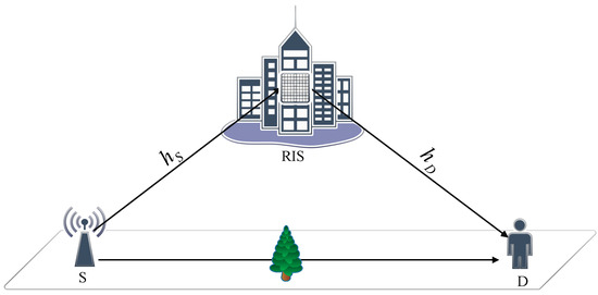
Figure 1.
Hybrid active–passive RIS for cooperative communication system.
The channel from S to HAPR is marked as , and that from HAPR to D is denoted as , where and . and are the amplitudes of the respective channel coefficients, which are mutually independent -m random variables (RVs), written as , . And and are the phase shifts of the respective channels.
2.1. Active Mode
During active mode, Switch 1 is “on”, Switch 2 is “off”, and all REs of HAPR are active elements. The transmit signal at S is x, with . In the meantime, the transmit power of S is defined as . The transmit signal from S that passes through the HAPR-assisted link reaches D, and the received signal at D is represented as follows:
where stands for the additive white Gaussian noise (AWGN) at D, and is the noise caused by the active RE. Hence, SNR at D could be expressed as
The first part is focused on the optimal phase design. Given that HAPR can dynamically change the incident signal’s phase for maximum SNR, from [14] we learned that the optimal phase design is as follows,
Referring to [19], the high altitude of S and HAPR lead to the presence of line-of-sight (LOS) links, and each RE has the same large-scale path loss, so the equal-gain amplification strategy is adopted in this paper as follows,
The reflection coefficient a is the second optimization problem we needed to pay attention to. The power consumption expression of the reflective amplifier in each active element was similar to that of the classical power amplifier,
where , , and are the power consumption of switching and control circuit, DC biased power consumption of each active element, and the output power of the reflective amplifier, respectively. As the active RIS amplification signal works in the linear region, the output power is associated with the incident power [19], which can be
In addition, is the reciprocal of the amplification efficiency. Considering the practical situation, RE has a pre-fixed power budget, which means that its amplification power is limited. At the same time, under active code, the reflection coefficient . Therefore, the optimization problem of the reflection coefficient is expressed as
The optimal reflection coefficient could be obtained as follows,
where . Because of realistic factors, the reflection coefficient is hardly equal to , so we adopt the more general case of in the follow-up research.
Under the condition of a high SNR, the typical calculation expression of the SNR at D is approximately:
2.2. Passive Mode
In passive mode, Switch 1 is “off”, Switch 2 is “on”, and all HAPR REs are passive. The received signal at D is represented as
The SNR at D is as follows when using the reflection coefficient and the aforementioned ideal phase design to maximize the SNR,
3. Performance Analysis
We initially analyze the performance of passive RIS and active RIS systems before investigating the performance of the hybrid active–passive RIS system, and compare the three. In this subsection, we derive the cumulative distribution functions (CDFs) for the end-to-end (e2e) SNR of the three RIS systems initially, and then derive the closed-approximation expression of outage probabilities by CDFs.
3.1. OP of the Full Active RIS System
For , , and according to and , we obtain the probability density function (PDF) and CDF of and , respectively, as follows,
where and . For the convenience of the subsequent calculation, we take and as the integer values here.
In the next step, using (17), and making and , the CDF of can be indicated as
The above equation can be further expressed as
By replacing with the integral variable t and bringing in the above integral, CDF of can be written as
Making use of ([28], (8.353.4)),
3.2. OP of the Full Passive RIS System
The outage probability of passive RIS can be written as
where . can be obtained by using the convolution formula. Its integral expression is processed with ([28], (3.471.9) (6.592.2)). The result is displayed as follows
where denotes the Meijer-G function with the order 2, 1, 1, and 3 [28].
The outage probability of passive RIS is
3.3. OP of the Hybrid Active–Passive RIS System
As previously mentioned, the HAPR system enables flexible switching of operating modes based on the channel conditions. That is, when the instantaneous SNR of all active REs exceeds that of all passive elements, RIS chooses to reflect signals using only active REs; conversely, it employs only passive REs for reflection. The e2e SNR of the hybrid HAPR system can be expressed as follows,
Then, the outage probability of the system can be written as
Theorem 1.
By a series of mathematical means, is provided by
where
, , , , and , , are the equipartition points of the original integration interval of , and respectively.
Proof of Theorem 1.
See Appendix A for details. □
4. Simulation Results
In the following section, we validate the derived formulas for mathematics utilizing Monte Carlo simulations and compare the outage probabilities of the three RIS systems. The system parameters are configured as follows: dBm, where and are the transmitting power and the total power of HAPR, respectively. The noise generated by the active RE is . The receiving noise is . The outage threshold is dB.
Firstly, we examine how the quantity of REs affects the passive RIS’s OP. For various values of N, the OP curves of the passive RIS-assisted system are displayed, as shown in Figure 2. It can be seen that the OP is smaller as increases, and the increase in N can also significantly reduce the OP and improve the system performance, a conclusion that is in perfect agreement with the theoretical values we have derived.
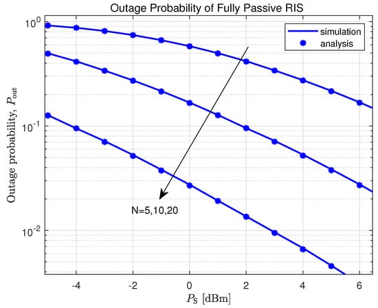
Figure 2.
OP versus for P−RIS with different numbers of N.
In Figure 3, we present the OP curves of the active RIS-assisted system under different N, It can be seen that the factors affecting the OP of the system are similar to those of the passive RIS-assisted system, in that the OP is reduced by increasing and N.
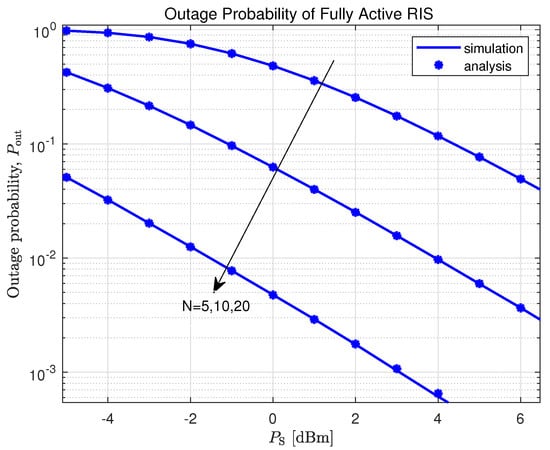
Figure 3.
OP versus for A−RIS with a different number of N.
In Figure 4, the OPs of the HAPR system are compared for . The results indicate that as and the quantity of REs rise, the OPs of the HAPR system continue to fall. Furthermore, we compare Figure 2, Figure 3, and Figure 4, which clearly reveal that HAPR requires a lower number of REs than A-RIS and P-RIS to achieve the same target OP value. This proves that HAPR requires a small physical size to achieve the desired communication target, which is advantageous in space-constrained situations. Compared with traditional RISs, HAPR has a wider range of application scenarios.
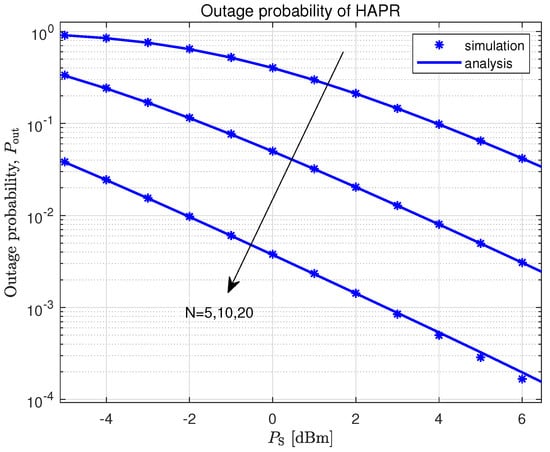
Figure 4.
OP versus for HAPR with different number of N.
In Figure 5, we compare the OP curves of the three RISs when and dBm. As the OP curves of the three RISs at and follow the same trend as at , except that the OPs are smaller, we only provide the simulations at here for the sake of overall aesthetics. Comparing these three curves, we find that the OP of the HAPR system is always lower than that of the A-RIS system and the P-RIS system, regardless of the value of . We also know from the figure that HAPR requires less than the two RISs to achieve the same OP, which means that the transmitter consumes less power and reduces the power consumption of the system, making it more energy efficient. Meanwhile, we also find an attractive phenomenon that the OP curves of A-RIS and P-RIS intersect near dBm. In other words, when is small, the OP of P-RIS is lower than that of A-RIS, in which case a better communication performance can be obtained by using P-RIS; however, when increases to greater than dBm, it is more sensible to use A-RIS to assist in signal transmission. This is because the array gain of the P-RIS is , while the gain of the active RIS is less than , so the SNR of the P-RIS is greater than that of the A-RIS when is small. As increases, A-RIS has enough power to amplify the signal, and this improves the gain, at which point A-RIS performs significantly better than P-RIS.
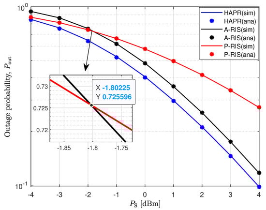
Figure 5.
OP of A−RIS, P−RIS, and HAPR under the same parameter setting .
5. Conclusions
In order to eliminate the “multiplicative fading” effect of passive RIS and the high-power consumption of active RIS, we provide a novel idea of hybrid active–passive RIS cooperative communication in this work. We arrive at the closed approximation expression for the outage probability of the HAPR system under the -m fading channel, obtain the number of HAPR reflective elements N as a function of the outage probability, and, by employing Monte Carlo simulations, verify that our mathematical expression is reliable. The simulation results demonstrate that HAPR has the advantages of a low power consumption, high gain, and high reliability compared with active and passive RIS.
Author Contributions
Conceptualization, W.W.; methodology, W.W.; software, W.W.; validation, W.W.; formal analysis, W.W.; investigation, W.W.; resources, W.W.; writing—original draft preparation, W.W.; writing—review and editing, W.W and K.S.; visualization, W.W.; supervision, K.S. All authors have read and agreed to the published version of the manuscript.
Funding
This work was supported, in part, by the National Natural Science Foundation of China under Grant 6190124, and, in part, by the Frontier Exploration Projects of Longmen Laboratory under Grant LMQYTSKT033.
Institutional Review Board Statement
Not applicable.
Informed Consent Statement
Not applicable.
Data Availability Statement
The data presented in this study are available on request from the corresponding author. The data are not publicly available due to privacy restrictions.
Conflicts of Interest
The authors declare no conflict of interest.
Abbreviations
The following abbreviations are used in this manuscript:
| RIS | Reconfigurable Intelligent Surface |
| HAPR | Hybrid Active–Passive Reconfigurable Intelligent Surface |
| RE | Reflecting elements Surface |
| OP | Qutage probability |
| CSI | Channel state information |
| CDF | Cumulative distribution functions |
| SNR | Signal-to-noise ratio |
Appendix A. The CDF Derivation of SNR for HAPR Systems
Let be the random variable x and be the random variable y, can be further written as
where D is the common region of curves and , the specific divisions are shown in Figure A1.
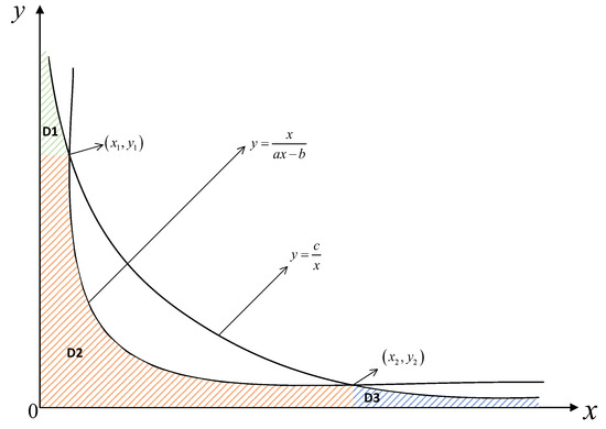
Figure A1.
OP versus for HAPR with a different number of N.
It can be found that coordinates and at the intersection of two curves are
The integral region in (A4) can be divided into three, and their double integrals are denoted, respectively, as follows,
where is the joint probability density of x and y, and as x and y are independent of each other, can be obtained directly from (13) and (14), as shown below
The integral with respect to x can be obtained by using Equations (3.381.1) and (8.353.6) in [28],
The second integral in (A12) can be replaced by
The integral of can be found using the Equation (3.471.9) in [28] as
In order to solve for the integral of , we employ the compound Simpson formula [29], which is expressed in a general form as follows,
where n is the number of equal parts of , is the step size, and interval points is used to construct the interpolation type product formulas, is the midpoint of the interval of .
Here, we split integral interval of (A14) into parts equally, the integral interval points are denoted as , where . Therefore, by substituting (A16) into the second integral of (A14), the approximate expression of the integral can be evaluated as follows,
where . Introduce (A13), (A15), and (A17) into (A12), the closed approximate expression for is
Moving forward, we evaluate the integral of the second region,
Using Equation (3.381.1) and Equation (8.353.6) in [28], we obtain the integral result with respect to y, which is
Likewise, the first integral in (A21) can be evaluated by using Equation (3.381.1) in [28], and the result of the integral is obtained as
Create a variable substitution for the second integral in (A21), that is, set , and rewrite it as
And then using the Equation (1.111) in [28],
By dividing into equal parts and using (A16), the approximate expression of the integral in (A25) can be obtained as
where . Bringing (A22), (A25), and (A26) into (A21), the approximate expression for is written as
Finally, we solve for the integral of the third region,
The integral solution of is the same process as that of . Using Equation (3.381.1) and Equation (8.353.6) in [28] first, we obtain
The second integral is equivalent to
Using the integral of in Equation (3.471.9) in [28], the solution is
References
- Córdoba, J.O.; Zarca, A.M.; Skármeta, A. Unmanned Aerial Vehicle Multi-Access Edge Computing as Security Enabler for Next-Gen 5G Security Frameworks. Intell. Autom. Soft Comput. 2023, 37, 2307–2333. [Google Scholar]
- Zhao, J.; Li, S.; Xu, X.; Yan, H.; Zhang, Z. Adaptive resource allocation of secured access to intelligent surface enhanced satellite–terrestrial networks with two directional traffics. AEU-Int. J. Electron. Commun. 2023, 170, 154746. [Google Scholar] [CrossRef]
- Boulogeorgos, A.-A.A.; AAlexiou, A. Ergodic Capacity Analysis of Reconfigurable Intelligent Surface Assisted Wireless Systems. In Proceedings of the 2020 IEEE 3rd 5G World Forum (5GWF), Bangalore, India, 10–12 September 2020; pp. 395–400. [Google Scholar]
- Yang, L.; Meng, F.X.; Wu, Q.Q.; da Costa, D.B.; Alouini, M.-S. Accurate Closed-Form Approximations to Channel Distributions of RIS-Aided Wireless Systems. IEEE Wirel. Commun. Lett. 2020, 9, 1985–1989. [Google Scholar] [CrossRef]
- Yang, L.; Meng, F.X.; Zhang, J.Y.; Hasna, M.O.; Renzo, M.D. On the Performance of RIS-Assisted Dual-Hop UAV Communication Systems. IEEE Trans. Veh. Technol. 2020, 69, 10385–10390. [Google Scholar] [CrossRef]
- P. de Figueiredo, F.A. Unlocking the Power of Reconfigurable Intelligent Surfaces: From Wireless Communication to Energy Efficiency and Beyond. Appl. Sci. 2023, 13, 11750. [Google Scholar] [CrossRef]
- Zhi, K.D.; Pan, C.H.; Ren, H.; Chai, K.K.; Elkashlan, M. Active RIS Versus Passive RIS: Which is Superior With the Same Power Budget? IEEE Commun. Lett. 2008, 10, 142–149. [Google Scholar] [CrossRef]
- Nor, A.M.; Fratu, O.; Halunga, S. Fingerprint Based Codebook for RIS Passive Beamforming Training. Appl. Sci. 2023, 13, 6809. [Google Scholar] [CrossRef]
- Luo, J.; Dai, H.; Wang, B.; Li, C. Design of Beamforming Algorithm for Ultra-reliable and Low-latency Communication in Heterogeneous Networks Based on IRS Assistance. J. Electron. Inf. Technol. 2023, 7, 2289–2298. [Google Scholar]
- Tao, Q.; Wang, J.W.; Zhong, C.J. Performance Analysis of Intelligent Reflecting Surface Aided Communication Systems. IEEE Commun. Lett. 2020, 24, 2464–2468. [Google Scholar] [CrossRef]
- Wu, Q.; Zhang, R. Intelligent Reflecting Surface Enhanced Wireless Network via Joint Active and Passive Beamforming. IEEE Trans. Wirel. Commun. 2019, 18, 5394–5409. [Google Scholar] [CrossRef]
- Liu, J.; Zhang, J.; Zhang, Q.; Wang, J.; Sun, X.H. Secrecy rate analysis for reconfigurable intelligent surface-assisted MIMO communications with statistical CSI. China Commun. 2021, 18, 52–62. [Google Scholar] [CrossRef]
- He, Z.-Q.; Yuan, X.J. Cascaded Channel Estimation for Large Intelligent Metasurface Assisted Massive MIMO. IEEE Wirel. Commun. Lett. 2020, 9, 210–214. [Google Scholar] [CrossRef]
- Hou, T.W.; Liu, Y.W.; Song, Z.Y.; Sun, X.; Chen, Y.; Hanzo, L. Reconfigurable Intelligent Surface Aided NOMA Networks. IEEE J. Sel. Areas. Commum. 2020, 38, 2575–2588. [Google Scholar] [CrossRef]
- Yang, L.; Guo, W.; Ansari, I.S. Mixed Dual-Hop FSO-RF Communication Systems Through Reconfigurable Intelligent Surface. IEEE Commun. Lett. 2020, 24, 1558–1562. [Google Scholar] [CrossRef]
- Yang, L.; Yan, X.Q.; da Costa, D.B.; Tsiftsis, T.A.; Yang, H.-C.; Alouini, M.-S. Indoor Mixed Dual-Hop VLC/RF Systems Through Reconfigurable Intelligent Surfaces. IEEE Wirel. Commun. Lett. 2020, 9, 1995–1999. [Google Scholar] [CrossRef]
- Do, T.N.; Kaddoum, G.; Nguyen, T.L.; da Costa, D.B.; Haas, Z.J. Aerial Reconfigurable Intelligent Surface-Aided Wireless Communication Systems. In Proceedings of the International Symposium on Personal, Indoor and Mobile Radio Communications (PIMRC), Toronto, ON, Canada, 5–8 September 2021; 32nd ed.. IEEE: Helsinki, Finland, 2021; pp. 525–530. [Google Scholar]
- Atapattu, S.; Fan, R.F.; Dharmawansa, P.; Wang, G.P.; Evans, J.; Tsiftsis, T.A. Reconfigurable Intelligent Surface Assisted Two-Way Communications: Performance Analysis and Optimization. IEEE Trans. Commun. 2020, 68, 6552–6567. [Google Scholar] [CrossRef]
- Long, R.Z.; Liang, Y.-C.; Pei, Y.Y.; Larsson, E.G. Active Reconfigurable Intelligent Surface-Aided Wireless Communications. IEEE Trans. Wirel. Commun. 2021, 20, 4962–4975. [Google Scholar] [CrossRef]
- Zhang, Z.J.; Dai, L.L.; Chen, X.B.; Liu, C.H.; Yang, F.; Schober, R.; Poor, H.V. Active RIS vs. Passive RIS: Which Will Prevail in 6G? IEEE Trans. Commun. 2023, 71, 1707–1725. [Google Scholar] [CrossRef]
- Huang, C.W.; Zappone, A.; Alexandropoulos, G.C.; Debbah, M.; Yuen, C. Reconfigurable Intelligent Surfaces for Energy Efficiency in Wireless Communication. IEEE Trans. Wirel. Commun. 2019, 18, 4157–4170. [Google Scholar] [CrossRef]
- You, C.S.; Zhang, R. Wireless Communication Aided by Intelligent Reflecting Surface: Active or Passive? IEEE Trans. Wirel. Commun. 2021, 10, 2659–2663. [Google Scholar] [CrossRef]
- Khoshafa, M.H.; Ngatched, T.M.N.; Ahmed, M.H.; Ndjiongue, A.R. Active Reconfigurable Intelligent Surfaces-Aided Wireless Communication System. IEEE Commun. Lett. 2021, 25, 3699–3703. [Google Scholar] [CrossRef]
- Liu, K.Z.; Zhang, Z.J.; Dai, L.L.; Xu, S.H.; Yang, F. Active Reconfigurable Intelligent Surface: Fully-Connected or Sub-Connected? IEEE Commun. Lett. 2022, 26, 167–171. [Google Scholar] [CrossRef]
- Wang, W.; Ji, B.; Song, K. RIS-Assisted Cooperative Transmission System with Adaptive Reflection Scheme. In Proceedings of the 2023 IEEE 6th International Conference on Electronic Information and Communication Technology (ICEICT), Qingdao, China, 21–24 July 2023; IEEE: Nanjing, China, 2023; pp. 1129–1134. [Google Scholar]
- Alexandropoulos, G.C.; Vlachos, E. A Hardware Architecture for Reconfigurable Intelligent Surfaces with Minimal Active Elements for Explicit Channel Estimation. In Proceedings of the ICASSP 2020-2020 IEEE International Conference on Acoustics, Speech and Signal Processing (ICASSP), Barcelona, Spain, 4–8 May 2020; IEEE: Barcelona, Spain, 2020; pp. 9175–9179. [Google Scholar]
- Taha, A.; Alrabeiah, M.; Alkhateeb, A. Enabling Large Intelligent Surfaces With Compressive Sensing and Deep Learning. IEEE Access 2021, 9, 44304–44321. [Google Scholar] [CrossRef]
- Gradshteyn, I.S.; Ryzhik, I.M. Table of Integrals, Series, and Products; Academic Press: Burlington, MA, USA, 2007; Volume 20, pp. 1157–1160. [Google Scholar]
- Abramowitz, M.; Stegun, I.A. (Eds.) Handbook of Mathematical Functions with Formulas, Graphs, and Mathematical Tables; National Bureau of Standards Applied Mathematics Series 55. Tenth Printing; Government Printing Office: Washington, DC, USA, 1972; p. 1076.
Disclaimer/Publisher’s Note: The statements, opinions and data contained in all publications are solely those of the individual author(s) and contributor(s) and not of MDPI and/or the editor(s). MDPI and/or the editor(s) disclaim responsibility for any injury to people or property resulting from any ideas, methods, instructions or products referred to in the content. |
© 2023 by the authors. Licensee MDPI, Basel, Switzerland. This article is an open access article distributed under the terms and conditions of the Creative Commons Attribution (CC BY) license (https://creativecommons.org/licenses/by/4.0/).