Gradient-Oriented Prioritization in Meta-Learning for Enhanced Few-Shot Fault Diagnosis in Industrial Systems

Abstract

In this paper, we propose the gradient-oriented prioritization meta-learning (GOPML) algorithm, a new approach for few-shot fault diagnosis in industrial systems. The GOPML algorithm utilizes gradient information to prioritize tasks, aiming to improve learning efficiency and diagnostic accuracy. This method contrasts with conventional techniques by considering both the magnitude and direction of gradients for task prioritization, which potentially enhances fault classification performance in scenarios with limited data. Our evaluation of GOPML’s performance across varied fault conditions and operational contexts includes extensive testing on the Tennessee Eastman Process (TEP) and Skoltech Anomaly Benchmark (SKAB) datasets. The results indicate a consistent level of performance across different dataset divisions, suggesting its utility in practical industrial settings. The adaptability of GOPML to specific task characteristics, particularly in environments with sparse data, represents a notable contribution to the field of meta-learning for industrial fault diagnosis. GOPML shows promise in addressing the challenges of few-shot fault diagnosis in industrial systems, contributing to the growing body of research in this area by offering an approach that balances accuracy and generalization with limited data.

1. Introduction

With the rapid advancement of industrial automation and informatization, fault diagnosis technology increasingly plays a pivotal role in ensuring the reliable operation of equipment and the safety of industrial systems [1]. Particularly in complex industrial environments, such as chemical, manufacturing, and energy sectors, the ability to accurately and swiftly identify and address faults is key to enhancing production efficiency and preventing accidents [2,3,4]. The recent surge in big data and Internet of Things (IoT) technologies has catalyzed the extensive deployment of sensors in industrial systems, resulting in a massive influx of data [5,6]. This data serve not only to record the operational status of equipment, but also to offer unparalleled opportunities for fault diagnosis. However, the high reliability of industrial equipment renders fault data relatively rare in comparison with data from normal operations, leading to a significant data imbalance, particularly in the context of few-shot fault diagnosis [7,8]. Given these circumstances, traditional machine learning and deep learning methods, which generally depend on abundant labeled data to train effective models, face substantial challenges [9,10,11,12]. Consequently, investigating potent few-shot learning techniques capable of accurately diagnosing faults in data-scarce environments has emerged as a crucial research area in industrial intelligence.

In the realm of few-shot learning, notable advancements and representative technologies or papers have emerged, particularly for addressing challenges in data-scarce environments. Methods such as data augmentation [13], synthetic data generation [14], transfer learning [15], self-supervised learning [16], and meta-learning [17] have been instrumental. These methods have demonstrated success in various fields, including object detection, image segmentation, and image classification, subsequently influencing fault diagnosis practices.

Focusing on the domain of fault diagnosis, few-shot learning has seen significant technological progress. Data augmentation techniques, particularly sampling methods and synthetic data generation, have been primarily employed to enhance fault data. Research in the field of rolling bearing fault diagnosis has shown that the use of compressed sensing for limited fault data augmentation can significantly improve diagnostic accuracy [18]. Furthermore, several studies have demonstrated that combining data augmentation with deep learning can effectively diagnose faults in rotating machinery [19,20], thereby enhancing both the precision and robustness of the diagnosis. Beyond data augmentation, alterations in model architecture have shown promise. Noteworthy among these is the development of a novel bidirectional gated recurrent unit (BGRU) for effective and efficient fault diagnosis [21]. Additionally, research has introduced few-shot fault diagnosis methods based on attention mechanisms, utilizing spectral kurtosis filtering and particle swarm optimization in conjunction with stacked sparse autoencoders [22]. The Siamese neural network, which learns through sample pair comparisons, is another innovative approach to the few-shot problem [23]. Transfer learning has played a significant role in enhancing the efficiency and accuracy of machine fault diagnosis, especially in cases where there are a scarcity of labeled data or low-precision sensors are utilized for data collection. Transfer learning has played a significant role in enhancing the efficiency and accuracy of machine fault diagnosis, especially in cases where there is a scarcity of labeled data or low-precision sensors are utilized for data collection [24,25]. However, these methods often require retraining the entire network for new tasks, limiting their practical adaptability in industrial settings. Additionally, varying operational conditions in practical engineering can diminish the effectiveness of these diagnostic methods under new circumstances. Hence, the need to identify fault categories across different working conditions remains a critical aspect of ongoing research in few-shot learning within fault diagnosis.

Meta-learning, as an adaptable approach to the few-shot problem, emphasizes the acquisition of learning capabilities rather than the learning process itself [26]. This strategy, pivotal in practical industrial applications, necessitates only minimal adjustments to accommodate new tasks [27]. Contrary to direct learning of a predictive mathematical model, meta-learning endeavors to understand the process of learning a generalized model [17]. Viewing feature extraction as direct data learning, the meta-learner gains insight by evaluating this process, enabling task completion with minimal samples. Among the various optimization-based meta-learning methods, model-agnostic meta-learning (MAML) seeks an initial parameter set sensitive to new tasks [28,29]. This approach allows for an enhanced performance following a gradient update on a small dataset of new tasks, demonstrating its potential in rapidly adapting to novel challenges.

In industrial systems, fault diagnosis relies on complex time-series signals gathered from equipment operating under varying conditions. The scarcity of fault samples and the diversity of working conditions pose challenges in discerning intricate fault information. To address this, the article introduces a novel gradient-oriented prioritization meta-learning (GOPML) approach. This method is designed to enhance the adaptability of meta-learning in recognizing few-shot fault conditions across diverse operational scenarios. GOPML optimizes knowledge adaptability, crucial for accurately identifying faults in data-rich yet sample-scarce environments.

The principal contributions of this work are encapsulated as follows:

• We introduce a novel gradient-oriented prioritization meta-learning (GOPML) approach that demonstrably mitigates overfitting in few-shot learning scenarios. By refining sensitive initialization parameters and harnessing the robust adaptability of knowledge, GOPML gains a distinct edge in tackling few-shot problems under varying operational conditions.
• This study advocates a strategic task sequencing strategy inherent to GOPML, bolstering the stability of the diagnostic performance amidst fluctuating operational conditions. The strategy draws inspiration from curriculum learning, methodically arranging tasks from the simplest to the most complex, thus endorsing a more stable, stepwise learning process. This structured learning trajectory is conducive to the development of a generalized knowledge representation, enhancing convergence efficiency with a reduced number of samples.
• The robustness of the GOPML algorithm is rigorously validated through extensive experiments on the Tennessee Eastman Process (TEP) and Skoltech Anomaly Benchmark (SKAB) datasets. The findings confirm GOPML’s adeptness in adapting to new categories in few-shot scenarios and its consistent diagnostic accuracy across varied working conditions. Comparative analysis further underscores the superiority of GOPML over contemporary state-of-the-art methods.

The article is organized to present a coherent exploration of the GOPML methodology in the following section, then empirical case studies are discussed to substantiate the method’s efficacy, culminating in a synthesis of insights in the concluding section.

2. Proposed Method

In this section, we delve into the proposed methodologies for meta-learning within the domain of fault diagnosis. Meta-learning stands as a transformative approach that empowers models to adapt quickly to new tasks, leveraging a small amount of data. Initially, we clarify the core principles and the task-oriented framework of meta-learning, providing clarity for its application in complex learning scenarios. The model-agnostic meta-learning (MAML) algorithm is presented as a foundational optimization-based meta-learning method. It has been pivotal in demonstrating how models can be tuned to new tasks efficiently using just a few iterations. Progressing further, we propose the gradient-oriented prioritization in meta-learning (GOPML) as an enhanced approach. GOPML refines the concept of task prioritization by incorporating gradient directions and magnitudes into the learning process, aiming to optimize the model’s performance across various tasks.

2.1. Rethinking the Meta-Learning Paradigm

In the deep learning domain, the standard approach necessitates voluminous datasets to effectively train models with a high predictive accuracy. This stands in stark contrast with the innate human ability to acquire and generalize new concepts from minimal exposure. An illustrative example of this is a child’s ability to differentiate between species, such as cats and dogs, after only a handful of observations. Meta-learning, or learning to learn, takes inspiration from this human cognitive trait and aims to emulate it within the realm of machine learning. This paradigm shift towards designing algorithms that require fewer examples to adapt and learn new skills embodies the core principle of meta-learning.

Meta-learning algorithms aspire to facilitate the acquisition of generalizable knowledge from a limited set of training examples, enabling the model to apply this knowledge to novel tasks. The objective is to construct a computational framework that allows machines to observe the strategies employed by various machine learning algorithms across a diverse set of tasks, assimilate the underlying patterns, and utilize this consolidated experience to solve new, unseen problems. Consider a machine learning classification task defined by a dataset $D=\{(x_1,y_1),\dots ,(x_n,y_n)\}$, where x denotes the input sample and y its corresponding label. The goal is to optimize the model parameters $\theta$, such that the model $y=f_{\theta }\left(x\right)$ minimizes the loss function over the dataset, formulated as follows:

$${\theta }^{*}=\underset{\theta }{\mathrm{argmin}}\mathcal{L}(D;\theta ,\omega )$$

(1)

Here, $\mathcal{L}$ represents the loss function and $\omega$ the learning strategy. In meta-learning, this is extended to a series of tasks $D_{\mathrm{train}}=\{(D_{\mathrm{train}}^1,D_{\mathrm{test}}^1),\dots ,(D_{\mathrm{train}}^m,D_{\mathrm{test}}^m)\}$, classified into training and testing phases, where the model’s efficacy is evaluated across these tasks using the expected loss:

$${\omega }^{*}=\underset{\omega }{\min }{\mathbb{E}}_{\tau \sim p\left(T\right)}\left[\mathcal{L}(D;\omega )\right]$$

(2)

In this equation, $p\left(T\right)$ refers to the distribution over all tasks and $\omega$ encapsulates the meta-knowledge, which is the knowledge representation that the model aims to generalize across different tasks.

The meta-learning framework employs a dual-layer learning structure. The meta-level (outer layer) is dedicated to learning a generalized knowledge representation ($\omega$), which evolves as it encounters new tasks. The task-level (inner layer) mirrors traditional machine learning models, focusing on updating the model with respect to individual tasks through training and testing. Every task, whether a training or testing instance, utilizes the meta-learner to facilitate a learning process that incorporates both the training data $D_{\mathrm{train}}$ and the testing data $D_{\mathrm{test}}$. To differentiate the primary dataset D used for the overall learning process from the meta-task specific data, we introduce the terms ‘support set’ for the training data and ‘query set’ for the testing data of the meta-tasks.

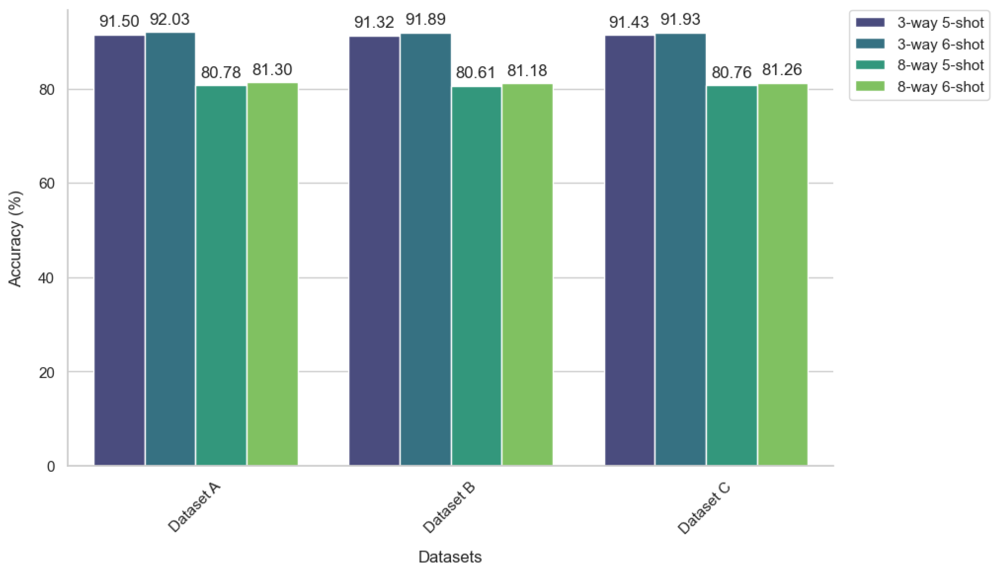
The meta-learner is trained on the support set and evaluated on the query set, with the objective of classifying samples into N categories. In an N-way classification, the meta-task is to classify data into N distinct categories. The term K-shot refers to the number of examples in the support set for each category, which results in $N\times K$ samples for training in each meta-task. Because of the random selection process, some overlap between the support and query sets of different tasks is expected, which does not compromise the model’s generalization capability due to the intrinsic fast adaptation feature of meta-learning. As long as there are distinctive differences in the training samples of each task, complete independence of tasks is not a prerequisite for effective meta-learning.

2.2. Model-Agnostic Meta-Learning (MAML) Framework

Building on the foundational concepts of meta-learning, the model-agnostic meta-learning (MAML) algorithm sets out to optimize the initialization parameters within the outer layer of the model. These parameters are crafted to be sufficiently broad-ranging, enabling the model to rapidly achieve an optimal performance on new tasks with limited data, following a minimal number of gradient updates. This process is pivotal from the standpoint of representational learning, as MAML seeks out internal representations that are universally applicable and easily transferable across a variety of tasks. The MAML algorithm undertakes the explicit training of parameters, representing the model with a function $f_{\theta }$, contingent upon the parameter $\theta$. The architecture of the model is delineated into two iterative loops: the inner loop focuses on specific task adaptation, and the outer loop targets generalization across tasks, with the parameter $\theta$ serving as the shared nucleus between them. Within the inner loop, the loss function for the subtask is calculated, precipitating an update of the parameters tailored to the new task. Post gradient descent, the model’s parameter $\theta$ is updated to ${\theta }_i^{\prime }$, as delineated by the equation:

$${\theta }_i^{\prime }=\theta -\alpha {\nabla }_{\theta }{\mathcal{L}}_T\left(f_{\theta }\right)$$

(3)

where $\alpha$ signifies the inner learning rate.

The outer loop encapsulates the meta-optimization process. It reassesses the inner loop’s optimized parameters ${\theta }_i^{\prime }$ against the novel task. This step facilitates the computation and subsequent update of the initial parameter $\theta$’s gradient:

$$\theta \leftarrow \theta -\beta {\nabla }_{\theta }\sum _{\tau \sim p\left(T\right)}{\mathcal{L}}_{\tau }\left(f_{{\theta }^{\prime }}\right)$$

(4)

Here, $\beta$ denotes the learning rate for the outer loop. The meta-learning model’s optimal parameters, tailored to the task distribution $p\left(T\right)$, emerge from the alternating optimization of the inner and outer loops. The meta-optimization’s overarching goal is to minimize the loss function across tasks:

$$\underset{\theta }{min}\sum _{\tau \sim p\left(T\right)}{\mathcal{L}}_{\tau }\left(f_{\theta }\right)=\sum _{\tau \sim p\left(T\right)}{\mathcal{L}}_{\tau }\left(f_{\theta -\alpha {\nabla }_{\theta }{\mathcal{L}}_T\left(f_{\theta }\right)}\right)$$

(5)

This iterative process, oscillating between the inner loop’s task-specific focus and the outer loop’s generalization-centric perspective, ensures the adaptability of the learned parameters to new, related challenges, embodying the quintessence of meta-learning: enabling a model to learn from the process of learning.

The MAML framework epitomizes the adaptability and flexibility required in rapidly evolving learning environments, demonstrating the profound potential of meta-learning algorithms to revolutionize the landscape of machine learning.

2.3. Gradient-Oriented Prioritization in Meta-Learning (GOPML)

In the domain of optimization-based meta-learning, precise initialization of model parameters forms the bedrock for swift and effective adaptation to new tasks. This pivotal step not only charts the trajectory of learning, but also determines the efficiency with which a model generalizes from a limited dataset. Hence, the strategic selection and sequencing of tasks are imperative in steering the learning process. Moving beyond random selection, a methodical approach to task organization exploits the inherent diversity and correlation among tasks to foster a more robust learning experience. Within this strategic framework, the arrangement of tasks is intentional, aiming to enhance the model’s adaptability to a variety of learning scenarios. Such an orderly engagement with tasks is designed to alleviate the uncertainties often linked with task relevance and complexity, seeking an equilibrium between reinforcing existing knowledge and integrating new, challenging concepts.

As we evolve towards a more sophisticated meta-learning paradigm, the emphasis shifts towards harnessing the subtle interplay of task characteristics. It is at this juncture that the gradient-oriented prioritization meta-learning (GOPML) algorithm distinguishes itself through the insightful analysis of gradient profiles from the loss function. The magnitude and direction of gradients are posited as crucial indicators of a task’s learning potential. The GOPML algorithm, through an integrated assessment of gradient information, purposefully orchestrates the learning process, concentrating on tasks anticipated to significantly enhance model performance. By quantifying gradient magnitudes and assessing the alignment of gradients across tasks, the learning path is tailor-made to ensure efficient and effective acclimatization to new challenges. Figure 1 encapsulates the sequential flow of the GOPML algorithm, demonstrating how each task is processed through the system. The diagram explicitly illustrates the gradient computation and the subsequent task prioritization, which are pivotal to the algorithm’s ability to adapt to and excel in new challenges. The orchestrated learning process, depicted in the figure, ensures that the most impactful tasks are prioritized, thus maximizing the model’s performance across a variety of tasks. The methodology unfolds as follows:

• Task Sampling: Tasks $T_i$ are sampled from a predetermined distribution $p\left(T\right)$, each comprising $N\times K$ data points to construct a dataset $D=\{x^{\left(i\right)},y^{\left(i\right)}\}$, correlating inputs x with labels y.
• Embedding Computation: Each task $T_i$ is processed to compute an embedding $E_{T_i}$, capturing its distinctive features.
• Gradient Computation and Task Prioritization: The gradient of the task-specific loss function $L_{T_i}$ with respect to model parameters $\theta$ is computed. The magnitude $G_{\mathrm{mag}}\left(T_i\right)$ and alignment $G_{\mathrm{align}}(T_i,T_j)$ of these gradients are assessed using:

  $$G_{\mathrm{mag}}\left(T_i\right)=\parallel {\nabla }_{\theta }{\mathcal{L}}_{T_i}\left(f_{\theta }\right)\parallel$$

  (6)

  $$G_{\mathrm{align}}(T_i,T_j)=\frac{{\nabla }_{\theta }{\mathcal{L}}_{T_i}\left(f_{\theta }\right)·{\nabla }_{\theta }{\mathcal{L}}_{T_j}\left(f_{\theta }\right)}{\parallel {\nabla }_{\theta }{\mathcal{L}}_{T_i}\left(f_{\theta }\right)\parallel \parallel {\nabla }_{\theta }{\mathcal{L}}_{T_j}\left(f_{\theta }\right)\parallel }$$

  (7)
  Tasks are then prioritized based on a score derived from their gradient magnitude and alignment:

  $$T_{\mathrm{score}}\left(T_i\right)=\gamma G_{\mathrm{mag}}\left(T_i\right)+\delta \sum _{j\ne i}{G}_{\mathrm{align}}(T_i,T_j)$$

  (8)
• Gradient Aggregation and Parameter Update: Gradients within each task cluster are aggregated based on prioritization scores, followed by a parameter update using gradient descent, modulated by step size hyperparameter $\alpha$.
• Global Parameter Update: After local updates, global adjustment of $\theta$ is performed using step size hyperparameter $\beta$, to integrate learning from all tasks.
• Model Evaluation: The model, with updated parameters $\theta$, is evaluated against new tasks, iterating until a satisfactory performance is achieved.

GOPML’s strategic framework for task selection and sequencing enhances the model’s ability to adapt and generalize. By focusing on the most impactful tasks, determined by gradient information, GOPML aims for more efficient learning and improved performance across diverse tasks. This approach, outlined in Algorithm 1, marks a shift towards a refined meta-learning paradigm, where the nuanced interplay of task characteristics is leveraged to amplify the learning potential, paving the way for enhanced generalization and mastery of new categories.

Algorithm 1 Gradient-oriented prioritization meta-learning (GOPML)

Require:  $p\left(T\right)$: distribution over tasks Require:  $\alpha ,\beta ,\gamma ,\delta$: step size and scoring hyperparameters

1: Randomly initialize $\theta$ 2: while convergence not achieved do 3:     Sample batch of tasks $T_i\sim p\left(T\right)$ 4:     for all $T_i$ do 5:           Generate task embedding $E_{T_i}$ using deep learning model 6:           Sample $N\times K$ datapoints $D=\{x^{\left(i\right)},y^{\left(i\right)}\}$ from $T_i$ 7:           Compute task-specific loss $L_{T_i}$ and gradient ${\nabla }_{\theta }{L}_{T_i}$ 8:           Compute gradient magnitude: $G_{\mathrm{mag}}\left(T_i\right)=\parallel {\nabla }_{\theta }{L}_{T_i}\parallel$ 9:     end for 10:   Perform clustering on $E_{T_i}$ to identify groups of similar tasks 11:   for each cluster do 12:         for all $T_i,T_j$ in the cluster do 13:               Compute gradient alignment: $G_{\mathrm{align}}(T_i,T_j)=\frac{{\nabla }_{\theta }{L}_{T_i}·{\nabla }_{\theta }{L}_{T_j}}{\parallel {\nabla }_{\theta }{L}_{T_i}\parallel \parallel {\nabla }_{\theta }{L}_{T_j}\parallel }$ 14:         end for 15:         for all $T_i$ in the cluster do 16:              Compute task score: $T_{\mathrm{score}}\left(T_i\right)=\gamma G_{\mathrm{mag}}\left(T_i\right)+\delta {\sum }_{j\ne i}{G}_{\mathrm{align}}(T_i,T_j)$ 17:         end for 18:         Aggregate gradients within the cluster based on $T_{\mathrm{score}}$ 19:         Compute parameters with gradient descent: ${\theta }^{\prime }=\theta -\alpha {\sum }_{T_i\in \mathrm{cluster}}{\nabla }_{\theta }{L}_{T_i}$ 20:     end for 21:     Update $\theta \leftarrow \theta -\beta {\nabla }_{\theta }{\sum }_{T_i\sim p\left(T\right)}{L}_{T_i}$ 22:     Evaluate model on unseen tasks and adjust $\theta$ if necessary 23: end while

3. Case Study

To evaluate the proposed GOPML approach, we applied it to the TEP dataset and SKAB dataset. The experiments conducted on these datasets aimed to assess the efficacy of the method in small sample scenarios and under fine-grained working conditions. The results demonstrate that the method exhibited a high accuracy in small sample fault diagnosis. Moreover, it showed a commendable performance in the transferability of fault diagnosis across various scenes.

3.1. TEP Dataset

3.1.1. Datasets Description

The Tennessee Eastman process (TEP), detailed by Downs and Vogel [30,31], is a comprehensive dataset widely studied in the diagnosis of chemical process faults. The process schematic is depicted in Figure 2. TEP comprises five main subsystems: a reactor, a condenser, a vapor–liquid separator, a recycle compressor, and a product stripper, among others. Each time-series sample in the TEP dataset contains 52 features, including 41 process measurements and 11 manipulated variables, recorded every three minutes. The TEP dataset includes a normal operation set with 500 samples and 21 fault conditions in the training subset, each with 480 samples. Correspondingly, the testing subset contains 960 samples per condition, with fault information being injected after 8 h of operation.

Because of the scant descriptions of the last six fault types in the dataset, only the first 15 fault categories are applied in the GOPML fault diagnosis.

Table 1. Fault types in the Tennessee Eastman Process evaluated by GOPML.

Variable	Fault State	Disturb
IDV1	A/C feed ratio, B composition constant	Step change
IDV2	B composition, A/C ratio constant	Step change
IDV3	D feed temperature	Step change
IDV4	Reactor cooling water inlet temperature	Step change
IDV5	Condenser cooling water temperature	Step change
IDV6	A feed loss	Step change
IDV7	C header pressure loss	Step change
IDV8	A, B, C feed composition	Random variants
IDV9	D feed temperature	Random variants
IDV10	C feed temperature	Random variants
IDV11	Reactor cooling water inlet temperature	Random variants
IDV12	Condenser cooling water valve	Random variants
IDV13	Reaction kinetics	Slow drift
IDV14	Reactor cooling water valve	Sticking
IDV15	Condenser cooling water valve	Sticking

This table lists the 15 fault types identified in the Tennessee Eastman Process (TEP) that were used to evaluate the GOPML algorithm.

elaborates on the 15 fault categories. The 15 scrutinized faults in TEP are unique from each other. Among these, Figure 3 displays the visualization of certain variables from normal samples and IDV2 samples in the training subset. Conventional diagnostic methods face challenges when there are no samples available for training the model for certain faults. Thus, the proposed GOPML approach to fault diagnosis is notably significant and practically applicable.

To align with the preprocessing requirements of the GOPML algorithm, the TEP dataset was methodically segmented using a sliding window methodology. The process utilized the windows of 40 consecutive data points, each reflecting a 2 h operational period, with a step size of 20 points to maintain temporal consistency. This arrangement ensured that each window adequately captured the complex dynamics of the process for a comprehensive learning experience. The GOPML algorithm then utilized this structured data to identify patterns and anomalies within the process. In total, each of the 15 fault categories was divided into 23 windows, yielding a collective 345 unique intervals for analysis. Additionally, for the testing subset, the initial 8 h of normal operational data were excluded, focusing the analysis on the subsequent samples where anomalies were introduced.

3.1.2. Experimental Setup

The N-way K-shot experimental protocol was adopted as a standardized approach for few-shot fault diagnosis. For the construction of a classification task, N categories were initially selected at random. Within each category, K examples were randomly drawn to form the support set, and Q examples to construct the query set. This sampling strategy was iterated to yield 10,000 training tasks and 100 testing tasks, ensuring broad validation of the GOPML algorithm. The learning process entailed a two-tier structure: the task-level inner layer and the meta-level outer layer, with learning rates for inner updates ($\alpha$) and outer learning ($\beta$) set at 0.01 and 0.001, respectively. Five inner update steps were designated for initial learning, followed by 10 steps for fine-tuning. This extensive task generation aimed to cover the TEP dataset’s diverse operating conditions and fault scenarios, enhancing the algorithm’s capability to generalize across varied learning contexts.

The base network for the TEP dataset was structured as a sequential model consisting of various layers designed to capture the temporal dependencies and features relevant for fault diagnosis, as delineated in

Table 2. Parameters of each module for the TEP dataset.

Layer Number	Module 1
L1	Conv1D (3, 64)
L2	ReLU
L3	BN
L4	Maxpool1D (2)
L5	LSTM (100)

. The parameter selection for this dataset, particularly regarding the Conv1D layer, was driven by the need to accurately model the dataset’s specific fault types and operational conditions. The smaller filter size in Conv1D was optimally suited for the TEP dataset’s requirements, where it is crucial to capture finer details of temporal sequences indicative of specific fault types. This precise parameter tuning enabled the GOPML algorithm to detect and classify a wide range of fault scenarios, thereby increasing the reliability and accuracy of fault diagnosis in the TEP dataset’s context. The network comprised five layers, forming an integral module of the architecture. Layer 1 (L1) featured a one-dimensional convolutional layer with 64 filters of size 3, processing the input data. This was succeeded by Layer 2 (L2), applying the rectified linear unit (ReLU) activation function for non-linearity. Subsequent layers performed batch normalization (BN) and max pooling operations, while the final layer integrated a long short-term memory (LSTM) network with 100 units, essential for capturing temporal sequence information in time-series data. The base learner’s structure for each module configuration within the network was uniformly designated as ‘Module 1’, with the last layer being a fully connected (FC) dense layer for the output layer, facilitating fault classification tasks, as presented in

Table 3. Structure of the base learner for TEP dataset.

Module Number	Base Learner
1	Module 1
2	Module 1
3	Module 1
4	Module 1
5	FC (Dense Layer)

.

3.1.3. Comparative Study on Few-Shot Fault Classification

In practical fault diagnosis, few-shot analysis often resorts to transfer learning methods. To benchmark against these methods, two deep neural networks renowned for their learning capabilities, namely VGG-11 [32] and Resnet-18 [33], were selected as the backbone architectures for knowledge transfer. During this process, fault data from the source domain were utilized to pretrain the base network, followed by fine-tuning with fault data from the target domain. Preliminary experiments indicated that fine-tuning the entire network achieved greater accuracy compared with merely adjusting the classifier. Hence, the experimental results of transfer learning were all based on the fine-tuning of the entire network. Crucially, to ensure a fair comparison, all comparative methods employed an N-way K-shot experimental setup.

In the domain of few-shot learning applications, the GOPML algorithm demonstrated its efficacy in fault diagnosis by optimizing the entire parameter set $\theta$ through a bi-level gradient descent strategy, as evidenced by the results presented in

Table 4. Fault classification results of the three methods.

Methods	3-Way Accuracy 5-Shot	3-Way Accuracy 6-Shot	8-Way Accuracy 5-Shot	8-Way Accuracy 6-Shot
Transfer VGG-11	84.20	89.84	74.14	79.78
Transfer Resnet-18	87.70	92.14	75.90	80.34
GOPML	93.53	97.48	84.01	86.59

. GOPML distinguished itself from traditional transfer learning methods that primarily focus on updating initialization parameters during the pretraining phase. Instead, GOPML employs a comprehensive update strategy across all tasks, thereby focusing on a more generalized initialization of parameters $\theta$ that facilitates rapid adaptation to new tasks.

The empirical results, as detailed in Table 4, underscore the significant accuracy improvements achieved by GOPML in few-shot fault diagnosis tasks. In particular, GOPML’s accuracy reached 93.53% and 97.48% in 3-way 5-shot and 6-shot tasks, respectively, and 84.01% and 86.59% in 8-way tasks for 5-shot and 6-shot scenarios. These figures substantially surpassed those of conventional transfer learning methods and highlighted the robustness of GOPML, especially when the number of training samples was limited. The improvements confirmed the effectiveness of the algorithm’s strategy in optimizing the parameters $\theta$ for better generalization across tasks.

3.1.4. Efficacy of Task Sequencing in GOPML

Task sequencing in GOPML aims to enhance the adaptability of knowledge through a more orderly and systematic learning approach. To validate the effectiveness of task sequencing in GOPML, a comparative analysis was conducted against the baseline algorithm, MAML, which did not incorporate task sequencing. Both algorithms shared a similar internal network architecture, with consistent training strategies and data partitioning. The distinctive factor between the two methods was the integration of task sequencing in GOPML’s external meta-learning layer. The classification results of fault diagnosis, illustrated in

Table 5. Fault classification results of GOPML and MAML on the TEP dataset.

Methods	3-Way Accuracy		8-Way Accuracy
	5-Shot	6-Shot	5-Shot	6-Shot
MAML Accuracy	90.32	92.10	80.75	81.92
GOPML Accuracy	92.53	97.48	84.01	86.59
MAML F1	91.22	92.70	81.13	82.60
GOPML F1	93.58	96.99	82.52	85.93
MAML precision	90.82	91.93	78.40	81.52
GOPML precision	92.01	96.16	81.15	85.31

, reflected the comparative study by varying the number of categories N and the samples per category K across different task setups. It was observed that GOPML surpassed MAML in classification accuracy in all task configurations. Notably, GOPML demonstrated substantial accuracy improvements in the 8-way 6-shot tasks, underscoring its superior learning performance with an increased number of categories and limited samples. This pronounced adaptability in complex few-shot scenarios established GOPML’s potential for real-world fault diagnosis applications.

In addition to accuracy, precision and F1 score were introduced for a more comprehensive evaluation. Precision measures the proportion of true positives to the sum of true positives and false positives, and the F1 score can be regarded as a weighted average of the model’s precision and recall. GOPML surpassed the baseline method on these metrics as well, except in the case of the 8-way 6-shot tasks, where GOPML’s performance was slightly lower, which may be due to the increased number of samples per task. Nevertheless, GOPML’s F1 score and accuracy remained outstanding when dealing with the 8-way 6-shot tasks. The performance of GOPML reflected its adaptability in complex few-shot scenarios, improving the performance because the ordering of tasks from easy to difficult was more in line with the acquisition process of meta knowledge. Standardizing the learning process of meta-learning will lead to better learning outcomes, such as making an orderly task-learning step. This step was conducive to the general knowledge representation learned from previous tasks, which helped the model adapt better to later tasks and thus achieve a better generalization performance.

During the training process, GOPML exhibited a higher resistance to performance degradation when tuning hyperparameters compared with MAML. Specifically, as training progressed, MAML’s accuracy rate rapidly reached saturation and then declined sharply, indicating a failure to achieve optimal training outcomes. In contrast, under identical hyperparameter settings, the training trajectory of GOPML remained stable throughout the training duration. This phenomenon is illustrated in Figure 4, which depicts the training process of both methods in a 3-way 6-shot setting.

Notably, the stair-like and progressive nature of GOPML’s training process ensured minimal difficulty variance between adjacent tasks. This approach effectively mitigated the risk of significant adverse impacts from earlier learned tasks on the subsequent ones. To further validate this characteristic, an extended experiment was conducted in an 8-way 6-shot scenario. The results, as shown in Figure 5, reinforced the consistency and robustness of GOPML’s training performance across more complex task configurations.

3.1.5. Effectiveness in Various Scenario Settings

To accurately identify faults within few-shot practical industrial contexts, it is not merely a question of overcoming the issue of insufficient samples, but also necessitates the capability for scene migration adaptability. When the training and testing sets comprised distinct categories, which were further delineated based on operational conditions, GOPML achieved a notably high precision. This demonstrates GOPML’s adaptability to various fault scenarios under differing operational conditions. However, given that the categories of both the training and testing sets were allocated randomly, it became impractical to ascertain whether the precision was a consequence of the faults in the testing set being readily identifiable. Therefore, to mitigate the influence of randomness in fault category allocation, we repeatedly conducted random selections of fault categories within the training and testing sets. Subsequent experiments were carried out across these varied data divisions (Datasets 1 to 4). The results, depicted in

Table 6. Fault classification results in different scenarios on the TEP Dataset.

Datasets	3-Way Accuracy		8-Way Accuracy
	5-Shot	6-Shot	5-Shot	6-Shot
Dataset 1	93.53	97.48	84.01	86.59
Dataset 2	92.41	96.21	83.58	85.38
Dataset 3	92.52	96.87	83.84	86.49
Dataset 4	93.35	96.37	83.91	85.82

and Figure 6, indicate that GOPML could secure favorable outcomes across different divisions, substantiating the stability of GOPML’s learning capabilities. The generalized knowledge acquired from certain faults could be employed to articulate the impacts on other faults.

3.2. SKAB Dataset

3.2.1. Datasets Description

The Skoltech Anomaly Benchmark (SKAB) [34], extensively utilized in industrial anomaly detection, encompasses a variety of subsystems within a simulated industrial environment. This includes an array of sensors, such as those for temperature, pressure, and flow rates. SKAB’s dataset comprises multiple features in each time-series sample, reflecting diverse sensor readings. It includes a baseline of normal operational data, alongside a series of artificially introduced anomalies to simulate industrial faults (Figure 7). These anomalies, present in both the training and testing subsets, are designed to replicate realistic conditions. SKAB consists of 34 time-series sets, with one anomaly-free set and 33 others transitioning from normal to anomalous states due to induced faults in the pumping system. The detection of anomalies, originating from various sources like valves and pumps, is the primary focus of this dataset. Despite their subtlety, as illustrated in Figure 8, these anomalies highlight the complexity of detection tasks. Originating from measurements of a single system, SKAB’s datasets are characterized by highly correlated channels, where anomalous data form a significant portion of each set.

In preparation for the application of the GOPML algorithm, the SKAB dataset was methodically preprocessed. This involved segmenting the dataset using a sliding window approach, where each window comprised 30 consecutive data points to adequately capture the dynamics of the industrial processes, with a step size of 15 points ensuring temporal overlap. Each of these windows was treated as an individual task, forming a structured dataset $D=\{x^{\left(i\right)},y^{\left(i\right)}\}$ that correlated inputs with their respective labels, vital for representing both normal operations and the 33 different types of anomalies present in SKAB. This task-specific formation allowed for nuanced pattern recognition and adaptation of the GOPML algorithm to the complexities of each anomaly type, enhancing its diagnostic capabilities. Additionally, clustering of these tasks based on feature similarity was conducted, aligning with GOPML’s methodology to facilitate more effective gradient aggregation and parameter updates within the algorithm.

3.2.2. Experimental Setup

The N-way K-shot experimental protocol was adopted for the fault diagnosis tasks within the SKAB dataset, in line with the standards of few-shot learning. For each classification task, N categories were randomly selected from the dataset, from which K examples were chosen to form the support set and Q examples to construct the query set. This sampling strategy resulted in the generation of 10,000 training tasks and 100 testing tasks, providing a comprehensive evaluation of the GOPML algorithm across a wide array of fault scenarios. The learning process was orchestrated across a two-tiered structure: the task-specific inner layer and the meta-level outer layer. The learning rates were set at $\alpha =0.01$ for task-level updates and $\beta =0.001$ for meta-level updates. The initial phase consisted of five inner update steps for preliminary adaptation, followed by 10 fine-tuning steps to refine the model’s performance.

The base learner’s architecture for the SKAB dataset was meticulously designed to capture temporal and feature dependencies crucial for accurate fault diagnosis. The choice of parameters for the SKAB dataset, such as the number and size of filters in the Conv1D layer, was specifically tailored to address the intricate fault patterns and operational variability characteristic of industrial processes. For instance, the larger filter size in Conv1D helped with capturing broader fault signatures, which was critical given the SKAB dataset’s emphasis on complex and varied fault conditions. This particular setup ensured that the GOPML algorithm could effectively discern subtle differences in fault patterns, a key requirement for the accurate diagnosis in diverse industrial scenarios. Each module, detailed in

Table 7. Parameters of each module for the SKAB dataset.

Layer Number	Module 2
L1	Conv1D (5, 64)
L2	ReLU
L3	BN
L4	Maxpool1D (2)
L5	Dropout (0.5)
L6	LSTM (100)

, begins with a Conv1D layer equipped with 64 filters of size 5, followed by a ReLU activation function for non-linearity introduction and batch normalization to stabilize the learning process. Module 2 incorporates a Maxpool1D operation to reduce dimensionality and a dropout layer with a rate of 0.5 to mitigate overfitting. The final layer in the sequence was an LSTM with 100 units, capturing long-term dependencies within the time-series data. The structure of these modules, as outlined in

Table 8. Structure of the base learner for the SKAB dataset.

Sequence Number	Base Learner
1	Module 2
2	Module 1
3	Module 2
4	Module 1
5	FC (Dense Layer)

, consists of alternating sequences of Module 1 and Module 2. The integration of an LSTM layer in the final step was particularly crucial for modeling the temporal sequences characteristic of the SKAB dataset’s time-series data, ensuring a comprehensive understanding of fault patterns over time.

3.2.3. Efficacy of Task Sequencing in GOPML

To verify the effectiveness of task sequencing, GOPML with task-sequencing was compared with the baseline algorithm MAML. The inner network architecture, the dataset’s partition, and the training strategy for both algorithms are consistent. The results of the fault diagnosis on the SKAB dataset are shown in

Table 9. Fault classification results of GOPML and MAML on the SKAB dataset.

Methods	3-Way Accuracy		8-Way Accuracy
	5-Shot	6-Shot	5-Shot	6-Shot
MAML Accuracy	89.30	90.41	78.95	80.07
GOPML Accuracy	91.50	92.03	80.78	81.30
MAML F1	85.62	86.85	77.00	78.22
GOPML F1	86.99	87.76	77.95	78.73
MAML precision	91.36	91.46	80.89	80.98
GOPML precision	93.50	93.07	82.08	81.64

and Figure 9. Under four different task settings, the accuracy rates of the proposed GOPML were 91.50%, 92.03% for the 3-way 5-shot and 6-shot settings, and 80.78% and 81.30% for the 8-way 5-shot and 6-shot settings, respectively. It can be seen that the meta-learning strategy with task sequencing could obtain better results than the one without sequencing. Moreover, when the number of samples in the support set was smaller, the accuracy improved more obviously. It verified the effectiveness of GOPML in few-shot scenarios. Besides accuracy, precision and F1 score were also introduced as evaluation indicators. As shown in Table 9, the F1 score and precision of GOPML were also excellent. To further explain the training process of GOPML, Figure 10 shows how the accuracy in a task changed as the update step increased. To optimize the efficiency of the experiment, the task-level update step in our experiments was set to 5. But, here, more intuitively, the task-level update step in Figure 9 is 10. It can be seen that the accuracy of the proposed GOPML method is improved more obviously and quickly.

3.2.4. Effectiveness in Various Scenario Settings

The experimental results mentioned above were obtained based on the premise that the categories for testing and training were distinct. It has been demonstrated that after learning, GOPML was capable of identifying faults through the use of initial parameter values and a limited number of adjustment steps when faced with new categories. The remarkable adaptability of GOPML to new categories underscored the method’s reliability in practical industrial scenarios. Moreover, to mitigate the influence of random division of data categories, three different random partitions on the SKAB dataset were also conducted. Subsequent experiments were carried out across these varied data divisions (Datasets A to C). The experiments executed under these divisions are summarized in

Table 10. Fault classification results in different scenarios on the SKAB dataset.

Datasets	3-Way Accuracy		8-Way Accuracy
	5-Shot	6-Shot	5-Shot	6-Shot
Dataset A	91.50	92.03	80.78	81.30
Dataset B	91.32	91.89	80.61	81.18
Dataset C	91.43	91.93	80.76	81.26

and Figure 10. These results show that GOPML maintained a balanced performance across different divisions, suggesting that regardless of how the fault categories were distributed, the learning ability of GOPML was consistently effective.

4. Discussion

This study introduced a novel gradient-oriented prioritization meta-learning (GOPML) algorithm, designed to enhance the efficiency and effectiveness of few-shot learning in fault diagnosis tasks. The methodological focus was on leveraging the intrinsic patterns embedded in industrial process data to enable robust fault diagnosis, using datasets such as TEP and SKAB. The GOPML algorithm demonstrated significant improvements over traditional methods in fault classification accuracy, precision, and F1 score, particularly in few-shot scenarios. The use of gradient-based task prioritization within GOPML has proven to be a key factor in its success, indicating that the magnitude and alignment of gradients are critical indicators of a task’s learning potential. This finding aligns with previous studies in meta-learning that have emphasized the importance of task selection and prioritization in improving learning outcomes. Another notable aspect of GOPML is its adaptability to different operational conditions and fault scenarios. The algorithm’s ability to maintain a balanced performance across various dataset divisions is indicative of its robustness and reliability in practical industrial contexts. This adaptability is crucial in fault diagnosis applications, where operational conditions can vary significantly.

The results also underscore the potential of GOPML in addressing the challenges posed by limited data availability in industrial settings. By optimizing the learning process through task sequencing and prioritization, GOPML has shown that it is possible to achieve high levels of diagnostic accuracy with a relatively small number of samples.

5. Conclusions

In this study, the gradient-oriented prioritization meta-learning (GOPML) algorithm has been proposed and evaluated for its applicability to few-shot learning within the realm of fault diagnosis. The algorithm’s structured approach to task prioritization, grounded in gradient analysis, contributes to its capability to adjust to a variety of fault scenarios, which is indicative of its potential utility in industrial settings. The analysis of the performance on the TEP and SKAB datasets demonstrates that GOPML can enhance diagnostic accuracy and precision, while offering a degree of generalization across different operational contexts. The findings suggest that GOPML could play a role in advancing intelligent diagnostic systems, especially in scenarios characterized by data scarcity and operational diversity. This study’s exploration into GOPML’s learning methodology, reflecting a capacity for rapid adaptation from limited data akin to human learning, may offer insights into meta-learning strategies. Looking forward, future research could extend to assess GOPML’s relevance in other fields beyond fault diagnosis and to refine the algorithm for improved handling of complex few-shot learning situations. The potential integration of GOPML with additional machine learning modalities also remains a promising avenue for future investigation, with the possibility of enhancing overall diagnostic methodologies.

References

1. Angelopoulos, A.; Michailidis, E.T.; Nomikos, N.; Trakadas, P.; Hatziefremidis, A.; Voliotis, S.; Zahariadis, T. Tackling faults in the industry 4.0 era—A survey of machine-learning solutions and key aspects. Sensors 2019, 20, 109. [Google Scholar] [CrossRef]
2. Bécue, A.; Praça, I.; Gama, J. Artificial intelligence, cyber-threats and Industry 4.0: Challenges and opportunities. Artif. Intell. Rev. 2021, 54, 3849–3886. [Google Scholar] [CrossRef]
3. Baalisampang, T.; Abbassi, R.; Garaniya, V.; Khan, F.; Dadashzadeh, M. Review and analysis of fire and explosion accidents in maritime transportation. Ocean. Eng. 2018, 158, 350–366. [Google Scholar] [CrossRef]
4. Bi, X.; Qin, R.; Wu, D.; Zheng, S.; Zhao, J. One step forward for smart chemical process fault detection and diagnosis. Comput. Chem. Eng. 2022, 164, 107884. [Google Scholar] [CrossRef]
5. Ahmed, S.F.; Alam, M.S.B.; Hoque, M.; Lameesa, A.; Afrin, S.; Farah, T.; Kabir, M.; Shafiullah, G.; Muyeen, S. Industrial Internet of Things enabled technologies, challenges, and future directions. Comput. Electr. Eng. 2023, 110, 108847. [Google Scholar] [CrossRef]
6. ur Rehman, M.H.; Yaqoob, I.; Salah, K.; Imran, M.; Jayaraman, P.P.; Perera, C. The role of big data analytics in industrial Internet of Things. Future Gener. Comput. Syst. 2019, 99, 247–259. [Google Scholar] [CrossRef]
7. Ren, Z.; Zhu, Y.; Liu, Z.; Feng, K. Few-shot GAN: Improving the performance of intelligent fault diagnosis in severe data imbalance. IEEE Trans. Instrum. Meas. 2023, 72, 3516814. [Google Scholar] [CrossRef]
8. Zhang, T.; Chen, J.; Li, F.; Zhang, K.; Lv, H.; He, S.; Xu, E. Intelligent fault diagnosis of machines with small & imbalanced data: A state-of-the-art review and possible extensions. ISA Trans. 2022, 119, 152–171. [Google Scholar] [PubMed]
9. Bansal, M.A.; Sharma, D.R.; Kathuria, D.M. A systematic review on data scarcity problem in deep learning: Solution and applications. ACM Comput. Surv. (Csur) 2022, 54, 1–29. [Google Scholar] [CrossRef]
10. Alzubaidi, L.; Bai, J.; Al-Sabaawi, A.; Santamaría, J.; Albahri, A.; Al-dabbagh, B.S.N.; Fadhel, M.A.; Manoufali, M.; Zhang, J.; Al-Timemy, A.H.; et al. A survey on deep learning tools dealing with data scarcity: Definitions, challenges, solutions, tips, and applications. J. Big Data 2023, 10, 46. [Google Scholar] [CrossRef]
11. Zhou, Y.; Wang, H.; Wang, G.; Kumar, A.; Sun, W.; Xiang, J. Semi-supervised Multiscale Permutation Entropy-enhanced Contrastive Learning for Fault Diagnosis of Rotating Machinery. IEEE Trans. Instrum. Meas. 2023, 72, 3525610. [Google Scholar] [CrossRef]
12. Zhen, D.; Li, D.; Feng, G.; Zhang, H.; Gu, F. Rolling bearing fault diagnosis based on VMD reconstruction and DCS demodulation. Int. J. Hydromechatron. 2022, 5, 205–225. [Google Scholar] [CrossRef]
13. Perez, L.; Wang, J. The effectiveness of data augmentation in image classification using deep learning. arXiv 2017, arXiv:1712.04621. [Google Scholar]
14. Figueira, A.; Vaz, B. Survey on synthetic data generation, evaluation methods and GANs. Mathematics 2022, 10, 2733. [Google Scholar] [CrossRef]
15. Zhuang, F.; Qi, Z.; Duan, K.; Xi, D.; Zhu, Y.; Zhu, H.; Xiong, H.; He, Q. A comprehensive survey on transfer learning. Proc. IEEE 2020, 109, 43–76. [Google Scholar] [CrossRef]
16. Jaiswal, A.; Babu, A.R.; Zadeh, M.Z.; Banerjee, D.; Makedon, F. A survey on contrastive self-supervised learning. Technologies 2020, 9, 2. [Google Scholar] [CrossRef]
17. Hospedales, T.; Antoniou, A.; Micaelli, P.; Storkey, A. Meta-learning in neural networks: A survey. IEEE Trans. Pattern Anal. Mach. Intell. 2021, 44, 5149–5169. [Google Scholar] [CrossRef]
18. Wang, D.; Dong, Y.; Wang, H.; Tang, G. Limited fault data augmentation with compressed sensing for bearing fault diagnosis. IEEE Sens. J. 2023, 23, 14499–14511. [Google Scholar] [CrossRef]
19. Li, X.; Zhang, W.; Ding, Q.; Sun, J.Q. Intelligent rotating machinery fault diagnosis based on deep learning using data augmentation. J. Intell. Manuf. 2020, 31, 433–452. [Google Scholar] [CrossRef]
20. Khan, A.; Hwang, H.; Kim, H.S. Synthetic data augmentation and deep learning for the fault diagnosis of rotating machines. Mathematics 2021, 9, 2336. [Google Scholar] [CrossRef]
21. Peng, P.; Zhang, W.; Zhang, Y.; Xu, Y.; Wang, H.; Zhang, H. Cost sensitive active learning using bidirectional gated recurrent neural networks for imbalanced fault diagnosis. Neurocomputing 2020, 407, 232–245. [Google Scholar] [CrossRef]
22. Zhang, X.; He, C.; Lu, Y.; Chen, B.; Zhu, L.; Zhang, L. Fault diagnosis for small samples based on attention mechanism. Measurement 2022, 187, 110242. [Google Scholar] [CrossRef]
23. Li, C.; Li, S.; Zhang, A.; Yang, L.; Zio, E.; Pecht, M.; Gryllias, K. A Siamese hybrid neural network framework for few-shot fault diagnosis of fixed-wing unmanned aerial vehicles. J. Comput. Des. Eng. 2022, 9, 1511–1524. [Google Scholar] [CrossRef]
24. Bhuiyan, M.R.; Uddin, J. Deep transfer learning models for industrial fault diagnosis using vibration and acoustic sensors data: A review. Vibration 2023, 6, 218–238. [Google Scholar] [CrossRef]
25. Zabin, M.; Choi, H.J.; Uddin, J. Hybrid deep transfer learning architecture for industrial fault diagnosis using Hilbert transform and DCNN–LSTM. J. Supercomput. 2023, 79, 5181–5200. [Google Scholar] [CrossRef]
26. Vilalta, R.; Drissi, Y. A perspective view and survey of meta-learning. Artif. Intell. Rev. 2002, 18, 77–95. [Google Scholar] [CrossRef]
27. Rajendran, J.; Irpan, A.; Jang, E. Meta-learning requires meta-augmentation. Adv. Neural Inf. Process. Syst. 2020, 33, 5705–5715. [Google Scholar]
28. Finn, C.; Abbeel, P.; Levine, S. Model-agnostic meta-learning for fast adaptation of deep networks. Int. Conf. Mach. Learn. 2017, 70, 1126–1135. [Google Scholar]
29. Fallah, A.; Mokhtari, A.; Ozdaglar, A. Personalized federated learning with theoretical guarantees: A model-agnostic meta-learning approach. Adv. Neural Inf. Process. Syst. 2020, 33, 3557–3568. [Google Scholar]
30. Downs, J.; Vogel, E. A plant-wide industrial process control problem. Comput. Chem. Eng. 1993, 17, 245–255. [Google Scholar] [CrossRef]
31. Bathelt, A.; Ricker, N.L.; Jelali, M. Revision of the Tennessee Eastman Process Model. IFAC-PapersOnLine 2015, 48, 309–314. [Google Scholar] [CrossRef]
32. Simonyan, K.; Zisserman, A. Very deep convolutional networks for large-scale image recognition. arXiv 2014, arXiv:1409.1556. [Google Scholar]
33. He, K.; Zhang, X.; Ren, S.; Sun, J. Deep Residual Learning for Image Recognition. In Proceedings of the IEEE Conference on Computer Vision and Pattern Recognition (CVPR), Las Vegas, NV, USA, 27–30 June 2016; pp. 770–778. [Google Scholar]
34. Katser, I.D.; Kozitsin, V.O. Skoltech Anomaly Benchmark (SKAB). Kaggle 2020. Available online: https://github.com/waico/SKAB (accessed on 8 May 2023).
Figure 1. Conceptual overview of GOPML for intelligent few-shot fault diagnosis.
Applsci 14 00181 g001
Figure 2. Flow chart of the Tennessee Eastman Process.
Applsci 14 00181 g002
Figure 3. The visualization of certain variables from normal samples and IDV2 samples in the training subset.
Applsci 14 00181 g003
Figure 4. The 3-way 6-shot accuracy in the outer loop.
Applsci 14 00181 g004
Figure 5. The 8-way 6-shot accuracy in the outer loop.
Applsci 14 00181 g005
Figure 6. Comparative fault classification accuracy across various scenarios in the TEP dataset.
Applsci 14 00181 g006
Figure 7. Front panel and composition of the water circulation, control and monitoring systems: 1—inverter; 2—a water pump; 3—emergency stop button; 4—electric motor; 5—compactRIO; 6, 7— solenoid valve; 8—a tank with water; 9—a mechanical lever for shaft misalignment. Not shown parts: vibration sensor; pressure meter; flow meter; thermocouple [34].
Applsci 14 00181 g007
Figure 8. Visualization of a fault scenario in SKAB—simulation of fluid leaks and fluid additions.
Applsci 14 00181 g008
Figure 9. Comparative accuracy in the inner loop for different task configurations.
Applsci 14 00181 g009
Figure 10. Comparative fault classification accuracy across various scenarios in the SKAB dataset.
Applsci 14 00181 g010