Quantitative Testing and Analysis of Non-Standard AEB Scenarios Extracted from Corner Cases

Abstract

Existing testing methods for Automatic Emergency Braking (AEB) systems mostly rely on standard-based qualitative analysis of specific scenarios, with a focus on whether collisions occur. To explore scenarios beyond the standard conduct, a comprehensive testing model construction and analysis, and provide a more quantitative evaluation of AEB performance, this study extracted three typical hazardous driving scenarios from the KITTI (The Automated Driving dataset was created by the Karlsruhe Institute of Technology in Germany and the Toyota Institute of Technology in the United States) naturalistic driving dataset using kinematic data. A DME (Data Missing Estimation) scene construction method was proposed, and these scenarios were simulated and reconstructed in PRESCAN (PRESCAN is an automotive simulation software owned by Siemens, Munich, Germany). A C-AEB (Curve-Automatic Emergency Braking) testing model was developed and tested based on simulations. Finally, a BCEM (Boundary collision evaluation model) was proposed to quantitatively evaluate AEB performance. The focus of the analysis was on the identified cornering scenario A (severely failed AEB scenario). A C-AEB testing model was constructed based on the DME scene construction method for this cornering AEB failure scenario, and it was evaluated using the BCEM. The study found that the average performance degradation rate (performance degradation rate refers to the ratio of AEB performance in the current scenario compared to the standard straightaway test) of the AEB system in this cornering scenario reached 75.44%, with a maximum performance degradation rate of 89.47%. It was also discovered that the severe failure of AEB in this cornering scenario was mainly caused by sensor system perception defects and limitations of traditional AEB algorithms. This fully demonstrates the effectiveness of our testing and evaluation methodology.

1. Introduction

Testing and verification of intelligent connected vehicles are crucial steps in the research and development of autonomous and assisted-driving vehicles and hold great significance for their development and implementation. Currently, autonomous driving testing is primarily categorized into virtual simulation testing, closed-site testing, and open-road testing based on the testing environment. Testing methods are further divided into use case-based testing, scenario-based testing, and public road testing. Scenario-based testing has emerged as a widely accepted approach within the industry for addressing the challenges of testing autonomous driving vehicles [1].

The term “scenario” originally found its application in the development of software systems that served to describe system usage, requirements, and environmental elements to facilitate the creation of more feasible systems [2,3,4,5,6].

However, in the realm of autonomous driving, a clear and unified definition of “scenario” is currently lacking. The concept of scenario was initially introduced to autonomous driving testing by Schieben [7]. Subsequently, Elrofa et al. proposed a definition of scenario as “the continuous variation of the dynamic environment surrounding the test vehicle within a specific time range, including the behavior of the test vehicle in that environment” [8]. Koskmies suggested that “a scenario is an informal description of a series of events that occur when a system performs a specific task” [9]. In the PEGASUS project, functional scenarios, logic scenarios, and concrete scenarios were introduced to account for the varying requirements of scenarios during the concept development, system development, and testing phases of autonomous driving product development [10].

To ensure sufficient diversity in the tested scenarios, it is crucial to establish a comprehensive test scenario library that encompasses a wide range of typical scenarios. Currently, several countries and institutions are involved in this endeavor. For instance, Germany’s PEGASUS and KITTI, the US’s NHTSA Automated Driving Test Framework project, UC Berkeley’s BDD100K, China’s “Kunlun Plan,” and Baidu’s Apollo Space are actively contributing to this effort [11]. These test scenario libraries draw data from three primary sources: real-world data, simulated data, and expert knowledge. Among these, real-world natural driving data stand out due to their abundant resources and widespread utilization.

Presently, hazardous scenario assessment methods can be broadly categorized into three types: time parameters, distance parameters, and deceleration parameters [12]. In the context of rear-end scenarios, the Time to Collision (TTC) is a commonly used indicator for evaluating the risk and likelihood of collisions [13,14,15]. However, as the relative speeds of the vehicles approach zero, the TTC value tends towards infinity. Hence, the reciprocal of TTC is typically employed to assess the severity of following-car scenarios [16]. Time Headway (THW) refers to the time interval between the host vehicle and the preceding vehicle, calculated by dividing the distance between them by the host vehicle’s speed. It represents the time required for the host vehicle to collide with the preceding vehicle along a straight line in the lane, assuming the preceding vehicle’s speed is zero. THW provides a measure of potential hazards and complements TTC in characterizing obvious dangers. It is commonly used to evaluate the severity of following-car scenarios and establish the alarm threshold for Advanced Driver Assistance Systems (ADAS) [17,18,19]. However, relying solely on TTC or THW has certain limitations when assessing the risk of following car scenarios.

TTC alone is insufficient for identifying hazardous scenarios in stable following processes with short distances and low relative speeds. Additionally, THW is influenced by factors such as vehicle type and driving ability and does not consider the preceding vehicle’s speed. To assess the danger level of the following car scenarios more accurately, it is necessary to consider additional factors, such as preceding vehicle speed, acceleration, and deceleration. Recent research has proposed new evaluation indicators like the Safety Distance Index (SDI) and Safety Time Index (STI), which comprehensively consider various factors in the following scenarios and have been validated in practical scenarios.

To address the limitations of TTC and THW, Kondoh et al. [20] proposed a method that calculates a danger perception coefficient by applying a reciprocal weighting approach. Furthermore, with the advancements in autonomous driving and artificial intelligence technology, various hazard assessment algorithms for hazardous driving conditions have been proposed. For example, Wang et al. [21] quantified the risk level using metrics such as maximum deceleration, average deceleration, and percentage decrease in vehicle kinetic energy. They also utilized classification and regression trees to study the relationship between the risk level and driver characteristics, surrounding vehicles, and road environment.

Satzoda [22] comprehensively evaluated the risk level between the host vehicle and the preceding vehicle during lane-changing processes by using the ratio of relative distance to safe distance. Fu et al. [23] developed a graded hazard assessment model for multiple key points during the vehicle braking process, utilizing an adaptive cuckoo search algorithm and BP neural network. The Responsibility-Sensitive Safety (RSS) model [24] proposed a minimum safe distance between the target vehicle and the following vehicle, assuming the worst-case scenario of the target vehicle suddenly applying the brakes. However, the RSS model’s conservative approach limits its use in risk assessment.

Professor Zhuxi Chan’s team from Tongji University proposed the use of time margin as an indicator for evaluating potential risks in the following scenarios [25]. Time margin enables the partitioning of the hazard area and earlier detection of rear-end collision risks, making it suitable for describing risks in stable following processes.

In summary, this article aims to extract typical hazardous scenarios from the KITTI dataset using a natural driving data extraction method. Inspired by the use of the five-point method for camera relative motion estimation [26], the five-point sampling method will be employed to simulate and reconstruct these typical hazardous scenarios in PRESCAN (8.5.0) and SIMULINK (R2020a). Our proposed boundary collision evaluation model will be used to quantitatively evaluate the performance of automatic emergency braking systems.

2. Extraction of Dangerous Scenes

2.1. Selection of Data Sets

The natural driving dataset plays a crucial role in scenario establishment. The KITTI dataset [27] was jointly established by the Karlsruhe Institute of Technology in Germany and the Toyota Technical Institute in the United States. The dataset’s primary collection platform includes two color cameras, two grayscale cameras, a 64-line 3D LiDAR, four optical lenses, and a GPS navigation system [28]. Here, we mainly use the vehicle’s motion information collected by GPS to filter the scenarios and use the images captured by the cameras to judge and reconstruct the scenarios.

2.2. Extraction of Dangerous Scenarios Based on Natural Driving Data

The method proposed by SHRP2 [28] and Zhu et al. [25] for screening hazardous driving conditions from naturalistic driving data was adopted in this study. The data were screened for hazardous driving conditions along both longitudinal and lateral dimensions, as shown in

Table 1. Screening conditions for dangerous conditions.

Trigger Class		Description
Longitudinal condition	Longitudinal deceleration	The longitudinal deceleration is less than or equal to −5 m/s2
	Longitudinal acceleration	The longitudinal acceleration is greater than or equal to 5 m/s2
	Longitudinal deceleration gradient	The velocity is higher than 5 m/s, and the longitudinal deceleration gradient is less than −10 m/s3
Transverse condition	Lateral acceleration	The absolute value is greater than 7 m/s2
	Lateral acceleration derivative	If the velocity is greater than 5 m/s, the absolute derivative of the lateral acceleration is greater than or equal to 10 m/s3

.

The method route for scenario screening is as follows (Figure 1):

The deceleration gradient can be used to measure the change in acceleration and, consequently, the speed at which the vehicle’s motion state changes. In the event of an emergency, the vehicle’s motion state undergoes significant changes within a short period. Here, the longitudinal deceleration gradient is primarily selected as the main screening criterion for hazardous scenarios.

The IMU data (IMU Data is the data collected by IMU sensors) in the KITTI dataset records the vehicle’s motion information at each timestamp, including dimensions, longitude, altitude, roll angle, pitch angle, yaw angle, longitudinal velocity, lateral velocity, x-axis acceleration, y-axis acceleration, and z-axis acceleration. According to the query results, the collection frequency of the KITTI dataset is 10 Hz, that is, the interval between every two timestamps is 0.1 s, from which the acceleration gradient corresponding to each timestamp can be calculated.

The KITTI dataset contains five folders: 2011_09_26, 2011_09_28, 2011_09_29, 2011_09_30, and 2011_10_03. Taking the 2011_09_26 dataset as an example, the screening was performed, and Figure 2 shows the screening results of the 2011_09_26 dataset.

The analysis results indicate that there are hazardous scenarios in this dataset that meet the longitudinal conditions. Detailed analysis was conducted for each sub-dataset, and the corresponding images were located to identify the corresponding scenarios.

Setting $\Delta a_x$ < −10 and $V_x$ > 5 as the criteria, screening was performed on the above five datasets, and the potential hazardous scenarios in this dataset were identified, as shown in

Table 2. Data of dangerous scenarios.

Serial Number	${\mathit{V}}_{\mathit{x}}$	${\mathit{a}}_{\mathit{x}}$	$\Delta {\mathit{a}}_{\mathit{x}}$	Owning Data Set
1	12.18	−0.26	−15.89	2011_09_26
2	10.3	0.48	−12.56	2011_09_26
3	5.00	−0.36	−12.6	2011_09_26
4	19.06	−0.04	−15.39	2011_09_26
5	6.59	1.28	−15.94	2011_09_26
6	9.72	0.65	−10.84	2011_09_28
7	7.54	−0.6	−14.24	2011_09_30
8	7.31	−0.71	−11.06	2011_09_30

:

Each data set is located through the time stamp, and after analysis, data from groups 4, 5, 6, 7, and 8 are eliminated. The corresponding scene has no traffic participants and belongs to the acceleration gradient change caused by terrain change.

Retrieve the images corresponding to sequence 1 based on the timestamp and collect all the images captured 5 s before and 5 s after the corresponding timestamp to reconstruct the scene. The image frames corresponding to the selected scenes are shown in Figure 3, Figure 4 and Figure 5.

3. Simulation Scenario Construction and Testing

PRESCAN is used to build the above scenario, and PRESCAN is combined with MATLAB (R2020a) to conduct AEB simulation.

3.1. Simulation Vehicle and AEB System Construction

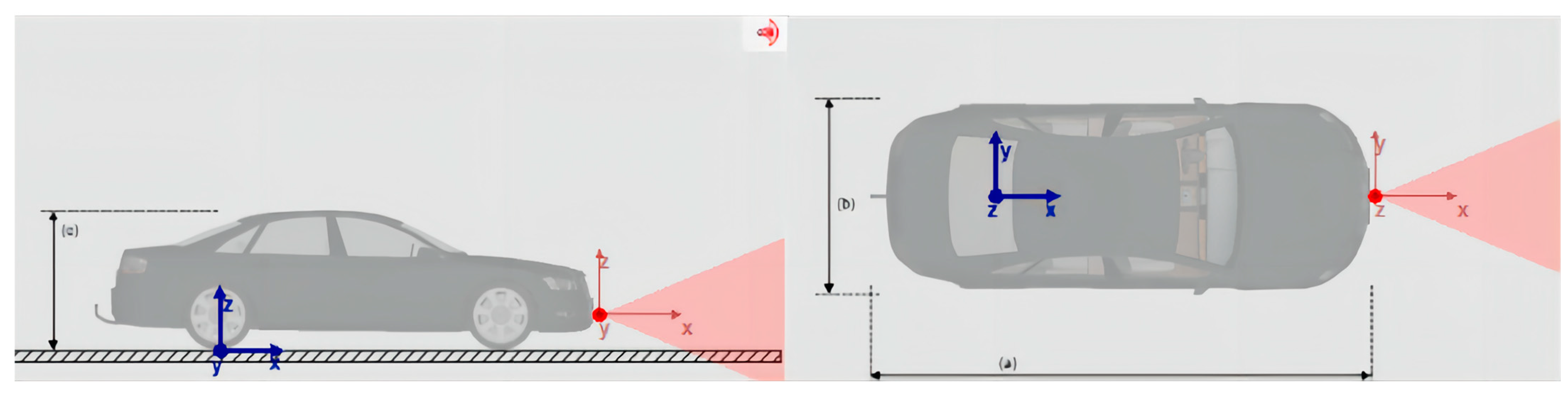
The Audi A8 has been selected as the test vehicle, with the Tesla Model 3 serving as the lead vehicle. To simulate millimeter-wave radar or lidar, two TIS sensors have been employed, with TIS1 designated for long-range sensing and TIS2 for blind-spot sensing. The coordinate origin is depicted in Figure 6, while

Table 3. Sensor parameters.

	Position	Scanning Mode	Sweep Frequency	Range of Perception	Perceived Angle
TIS1	(3.94, 0, 0.37)	Line scan	25 Hz	150 m	9°
TIS2	(3.94, 0, 0.37)	Line scan	25 Hz	30 m	80°

outlines the sensor positions, scanning methods, scanning frequencies, sensing ranges, sensing angles, and other pertinent parameters.

In Simulink, we created a simulation of an ego car. The AEB system model, driver model, sensor model, ego vehicle model, and tire model are all built-in models provided by PRESCAN.

Here, we establish data connections between different modules to form a complete AEB system. The ego vehicle model outputs the relevant kinematic data of the vehicle, including the speed and yaw rate, which are then fed into the path tracking module. This module utilizes PID control to enable the vehicle to track a pre-determined motion trajectory, and subsequently outputs information such as throttle opening to the vehicle’s dynamic model and tire model, thereby simulating realistic vehicle behavior.

The AEB system module receives outputs from both the sensor model and the driver model. The main information includes the speed and yaw angle of the ego vehicle, as well as the distance and angle of the target objects detected by TIS1 and TIS2, the status signals and brake signals output by the driver model, and the engine speed. The AEB system is structured as a three-level system, using the Time-to-Collision (TTC) as the warning threshold. When TTC reaches 2.6 s, the driver is alerted. When TTC reaches 1.6 s, 40% brake pressure is applied. When TTC reaches 0.6 s, full brake pressure is applied. The actions taken at different TTC warning levels are summarized in

Table 4. AEB actions of different warning signals.

Warning Flag	1.6 s Flag	0.6 s Flag	Action
0	0	0	Do nothing
0	0	1	Do nothing
0	1	0	Apply 40% braking force
0	1	1	Apply Max braking force
1	0	0	Apply braking force put on by the driver
1	0	1	Apply braking force put on by the driver
1	1	0	Apply 40% braking force
1	1	1	Apply Max braking force

.

The difference between the Autonomous Emergency Braking (AEB) system and the Pre-emptive Braking System needs to be discussed here. The differences between them are as follows:

• Triggering Mechanism: The AEB system automatically engages the brakes when the vehicle detects an imminent collision. It utilizes sensors and algorithms to monitor obstacles ahead and proactively initiates braking maneuvers when collision risks are identified. On the other hand, the Pre-emptive Braking System applies braking force in advance when potential collisions or hazardous situations are predicted, aiming to reduce collision risks.
• Active vs. Passive Operation: The AEB system is an active safety system that autonomously performs emergency braking without reliance on driver input. In contrast, the Pre-emptive Braking System typically functions as an auxiliary feature, providing warnings or assisting with braking but still requiring appropriate driver actions to avoid collisions.
• Operational Strategy: The AEB system’s strategy is focused on minimizing the severity of collisions by swiftly engaging emergency braking once collision risks are detected. Conversely, the Pre-emptive Braking System employs a strategy of applying braking force in advance to prevent potential collisions, offering additional safety assistance to the driver.

3.2. Scenario Test and Analysis

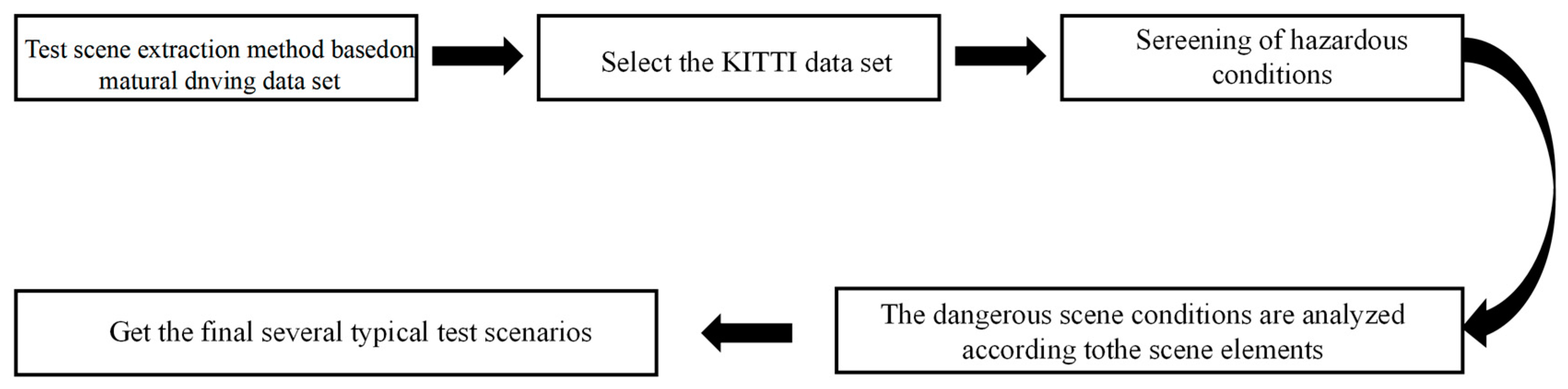
Our proposed methods will be discussed here, including 1. Data Missing Estimation (DME) Scene architecture method, 2. C-AEB (curve AEB) Test method, 3. Boundary collision evaluation model (BCEM) Evaluation model.

We proposed the DME (Data Missing Estimation) method for scene construction, which addresses the lack of accurate data on the positions and distances of relevant traffic participants in the natural driving dataset. Additionally, we propose the C-AEB (Curve-AEB) model for non-standard AEB testing in curved road scenarios and the BCEM (Boundary collision evaluation model) for assessing non-standard AEB performance specifically in curved road scenarios. Subsequently, we create the scenarios in PRESCAN and develop the AEB system using SIMULINK in MATLAB. Finally, we conduct simulation testing and perform evaluation analysis.

• DME (Data Missing Estimation) Scene architecture method

Here, we will construct the selected image scenes in PRESCAN and develop an experimental plan. Since dangerous scenarios are continuous in time, and the natural driving dataset lacks accurate data on the positions and distances of relevant traffic participants, the focus of the scenario testing is on the performance of the AEB system in this scenario rather than the performance of a specific test case within the scenario. Therefore, we assume that the positions of the ego vehicle and obstacle vehicles within the feasible driving area are uniformly distributed in the same scenario. Drawing inspiration from the commonly used 5-point sampling method in biology, we propose a “Data Missing Estimation” for AEB system testing to test the overall scenario. The specific approach is as follows:

For scenarios where the ego vehicle and obstacle vehicle intersect (such as at intersections or merging lanes), we will use the intersection point of the lane centerlines as the collision center point. Two collision points will be arranged equidistantly on either side of the collision center point, resulting in a total of five collision points (the collision point here refers to the coordinate point at which the car collides with the car in front of it in the current scene).

For curved road scenarios, since the trajectories of the ego vehicle and obstacle vehicle overlap, we will divide the curved road into five segments and place a collision point at the center of each segment, resulting in a total of five collision points.

For straight road scenarios, we will set five collision points at equal distances along the road.

2.

C-AEB (curve AEB) Test method

Based on the CN-cap testing standard, we propose a testing methodology specifically designed for curved road scenarios, called C-AEB (Curve-Aware Emergency Braking). In this methodology, the test cases for each scenario are divided into three categories: Lead Vehicle Stationary (CCRs), Lead Vehicle Slow Moving (CCRm), and Lead Vehicle Decelerating (CCRb).

Unlike the testing standard, the Lead Vehicle Stationary category involves the lead vehicle being stationary at five different points. The test vehicle starts from 0 km/h and incrementally increases its speed by 5 km/h until a collision occurs.

In the Lead Vehicle Slow Moving category, the lead vehicle travels at speeds of 10 km/h, 20 km/h, and 30 km/h. The starting position of the test vehicle is not fixed but remains outside the perception range. The final collision point is set at the aforementioned five points.

For the Lead Vehicle Decelerating category, the setup is similar to the Lead Vehicle Slow Moving category. However, there are no restrictions on the initial speed and position of the lead vehicle, as long as it is outside the perception range. Only the final collision point is set at the aforementioned five points.

3.

BCEM (Boundary collision evaluation model) Evaluation model

We propose a boundary collision evaluation model referred to as BCEM (Boundary Collision Evaluation Model). Based on the analyzed physical quantities, we can define the scenario type as T, the stationary lead vehicle scenario as $A_1$, the slow-moving lead vehicle scenario as $A_2$, and the decelerating lead vehicle scenario as $A_3$. The initial speed of the lead vehicle is $V_0$, the safety boundary speed is $V_r$, the maximum safety boundary collision speed is $V_{rmax}$, and the maximum safety boundary collision speed for a straight road is $V_{rdmax}$. The performance decay rate is defined as $\varnothing$, and the AEB system implemented here is designed for straight paths, which have been shown to have the best performance in the experiments, we will use the maximum safety boundary collision speed for the straight road as the evaluation benchmark. The maximum safety boundary speed refers to the minimum collision speed corresponding to the test of five collision points in this scenario, and the minimum speed is taken as the evaluation of its safety performance, because for the AEB system, there is the possibility of unsafe collision, so the name of the boundary is also introduced here. The maximum safety boundary collision speed refers to the speed from 1 km/h on the straight road until the collision occurs. The performance decay rate $\varnothing$ is defined as Equation (1), and the average performance decay rate ${\varnothing }_m$ is defined as Equation (2) to describe the average performance decay of the three test cases: $A_1$, $A_2$, $A_3$, (${\varnothing }_{A1},{\varnothing }_{A2},{\varnothing }_{A3}$ refers to the attenuation rate of the AEB system in the three test scenarios A1, A2, and A3, respectively) in this scenario.

$$\varnothing =\frac{V_{rdmax}-V_{rmax}}{V_{rdmax}}$$

(1)

$${\varnothing }_m=\frac{{\varnothing }_{A1}+{\varnothing }_{A2}+{\varnothing }_{A3}}{3}$$

(2)

We will now proceed to construct experimental cases and conduct simulations for various real-world scenarios.

3.2.1. A Scenario Construction Test and Analysis

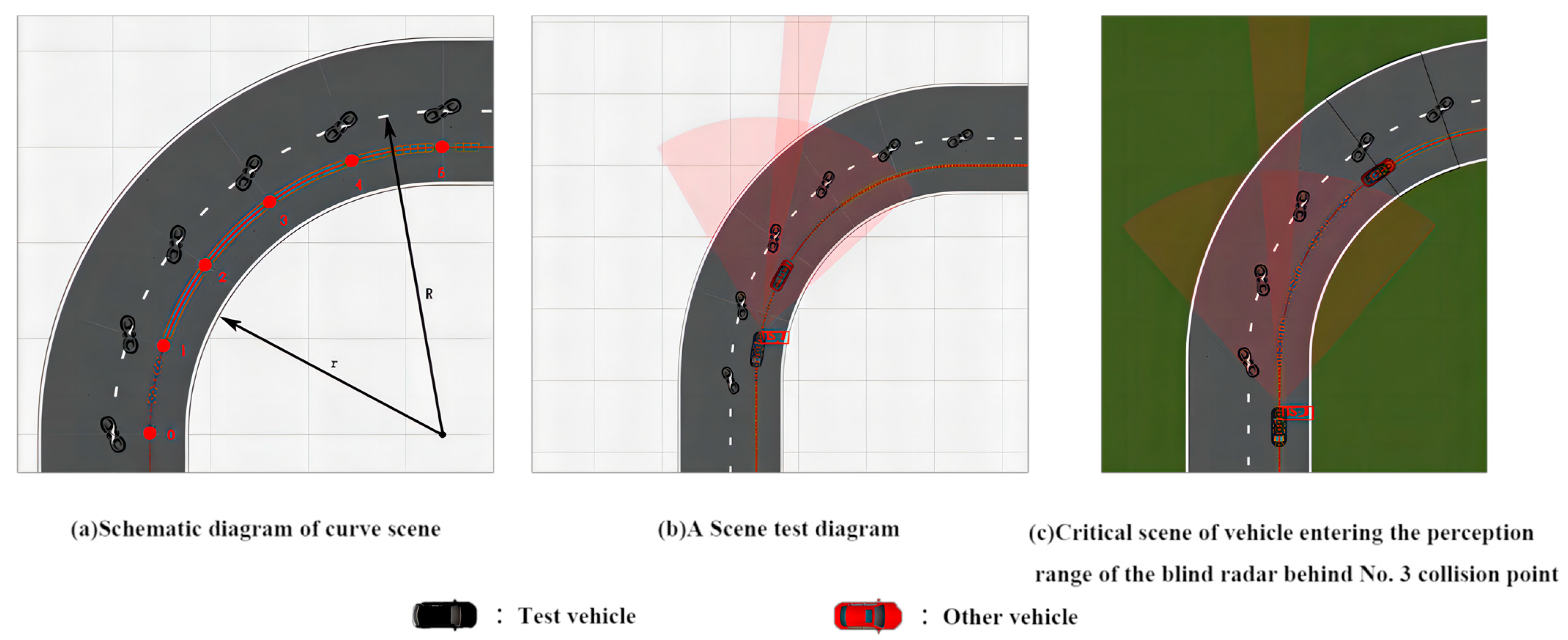
According to Chinese highway standards [29], the radius of a road is 30 m, and the width of a single lane is 3.75 m. We will construct a one-way two-lane road in PRESCAN, as shown in the Figure 7, with R = 33.75 m and r = 30 m. We will divide the 90-degree curve into five segments, with each segment having a curvature of 18 degrees, and set collision points 1, 2, 3, 4, and 5.

Concerning the CN-cap testing standard, we will design the experiment and divide the test cases for this scenario into three categories: stationary lead vehicle, slow-moving lead vehicle, and decelerating lead vehicle. To quantitatively describe the performance boundaries of the AEB system in this scenario, we define the maximum ego vehicle speed at which no collision occurs as the collision boundary speed. We will construct test cases for each of the three lead vehicle scenarios: stationary, slow-moving, and decelerating.

• Stationary lead vehicle:

The lead vehicle will be placed at collision points 1 to 5, and the test vehicle will start from a distance of 200 m from the beginning of the curve to realistically simulate actual traffic scenarios. The test will be conducted at speeds increasing in increments of 5 km/h from 5 km/h to 100 km/h. The collision boundary speed when there is no collision at collision point 0 will be used as the reference data for comparison. The experimental results are shown in the table below (

Table 5. Static scene test results of vehicle in front of curve.

Collision Point	Boundary Impact Velocity (km/h)
0	95
1	40
2	40
3	35
4	40
5	40

, Figure 8):

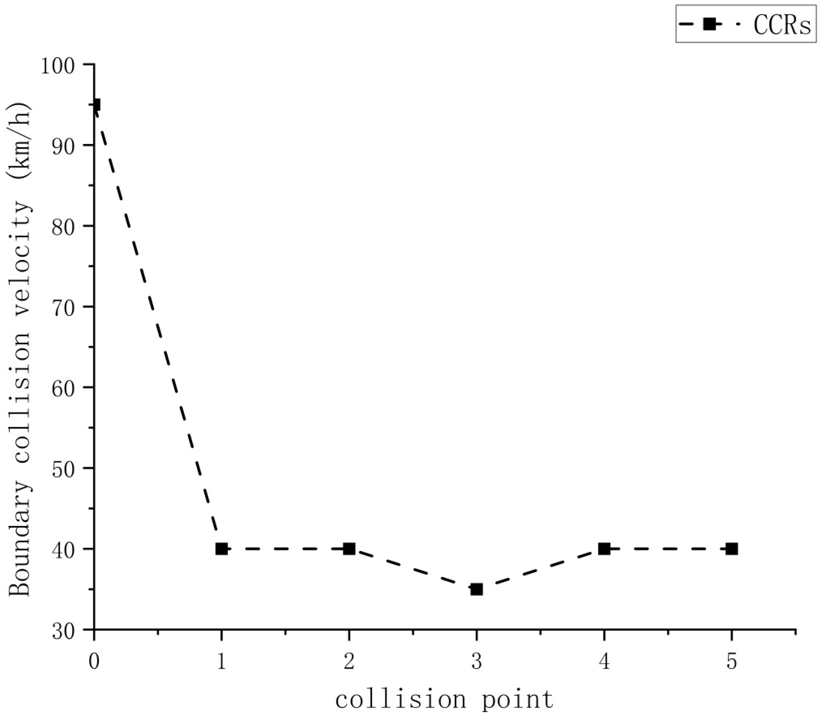
As shown in Table 5, the experimental results indicate that the AEB system’s boundary speed is higher at collision point 0 while it is lower at the collision points on the curved road, with the lowest value at collision point 3 at 35 km/h.

2.

Slow-moving lead vehicle:

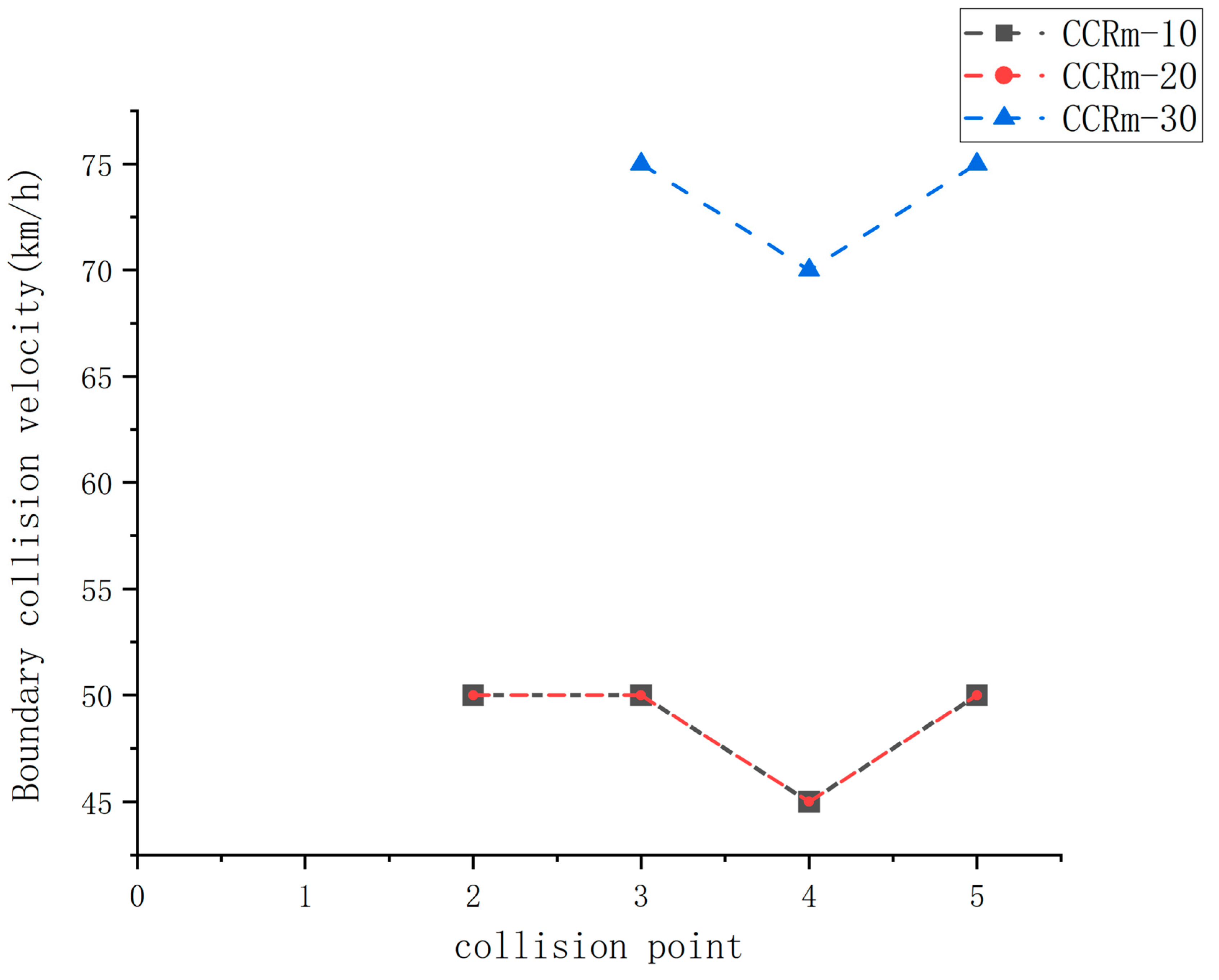
According to Chinese regulations, the speed limit for curved sections of urban roads is 30 km/h. Thus, we will set the lead vehicle’s speed to 10, 20, and 30 km/h, with the starting point at 0. Five collision points will be set at positions 1 to 5 relative to the lead vehicle, and the speed range of the test vehicle will be set to 10–80 km/h. The experimental results are shown in the table below (

Table 6. Test results of slow driving in front of curve.

Ahead Speed	Collision Point	Boundary Impact Velocity (km/h)
10	1	/
	2	50
	3	50
	4	45
	5	50
20	1	/
	2	50
	3	50
	4	45
	5	50
30	1	/
	2	/
	3	75
	4	70
	5	75

Note: “/” indicates that no collision occurred within the set speed range.

, Figure 9):

3.

Decelerating lead vehicle:

In this scenario, the conditions will be the same as the slow-moving lead vehicle scenario, except that the lead vehicle’s speed will be set to 0 at all collision points. The initial speeds of the lead vehicle will still be set to 10 km/h, 20 km/h, and 30 km/h, respectively, for testing. The experimental results are shown in the table below (

Table 7. Test result of front vehicle deceleration scene in curve.

Ahead Speed	Collision Point	Boundary Impact Velocity (km/h)
10	1	/
	2	40
	3	40
	4	40
	5	45
20	1	/
	2	40
	3	40
	4	40
	5	40
30	1	/
	2	40
	3	40
	4	40
	5	40

Note: “/” indicates that no collision occurred within the set speed range.

, Figure 10):

The statistical representation of test results for scenario A is shown in Figure 11, for the stationary lead vehicle scenario, collision point 0 is located at the end of the straight road. When driving on a straight road, the AEB system’s boundary collision speed is 95 km/h. After entering the curved road, collision point 3 spends more time in the blind zone of the sensors and can only be sensed by the supplementary radar at the turning point. Therefore, its boundary collision speed initially increases with the turning angle but then begins to decrease again after exiting the curve. Figure 7c shows a critical scenario where the test vehicle enters the supplementary radar detection range at collision point 3 while the lead vehicle is present.

For the slow-moving lead vehicle scenario, the boundary collision speed for the 10 km/h scenario is 45 km/h, the boundary collision speed for the 20 km/h scenario is 60 km/h, and the boundary collision speed for the 30 km/h scenario is 70 km/h. As the lead vehicle speed increases, the safety boundary of the AEB system also increases.

Since this AEB system is designed based on the TTC (Time-to-Collision) principle, the most important factors affecting the system’s response are the speeds of the lead and test vehicles. Therefore, we can use the difference between the test vehicle’s boundary speed and the lead vehicle’s slow-moving speed to measure the system’s response boundary. Based on safety principles, we will take the minimum value of the five collision points as the boundary collision speed for safety. The safety boundary collision speeds for the 10 km/h, 20 km/h, and 30 km/h scenarios are 35 km/h, 25 km/h, and 40 km/h, respectively. Therefore, the range of the AEB system’s safety boundary collision speed for the curved road in this scenario is 25–40 km/h. Based on safety principles, the maximum safety boundary collision speed for the AEB system in this scenario is the minimum value, which is 25 km/h.

For the decelerating lead vehicle scenario, the boundary collision speeds for the 10 km/h, 20 km/h, and 30 km/h scenarios are 30 km/h, 20 km/h, and 10 km/h, respectively. Based on safety principles, the maximum safety boundary collision speed for the AEB system in this scenario is the minimum value, which is 10 km/h.

The data of each experimental case are summarized in

Table 8. Experimental data of Scene A.

$\mathit{T}$	${\mathit{V}}_0$	${\mathit{V}}_{\mathit{r}}$	${\mathit{V}}_{\mathit{r}\mathit{m}\mathit{a}\mathit{x}}$	$\varnothing$	${\varnothing }_{\mathit{m}}$	${\mathit{V}}_{\mathit{r}\mathit{d}\mathit{m}\mathit{a}\mathit{x}}$
$A_1$	0	35	35	63.16%	75.44%	95
$A_2$	10	35	25
	20	25		73.68%
	30	40
$A_3$	10	30	10
	20	20		89.47%
	30	10

Note: The unit of speed in km/h.

.

The data shows that the average performance decay rate ${\varnothing }_m$ of the AEB system in this scenario is 75.44%. The performance decay rate $\varnothing$ of the AEB system in the decelerating lead vehicle scenario reaches 89.47%. In this situation, the AEB system is essentially ineffective, making this scenario one of the more dangerous scenarios for the AEB system.

3.2.2. B Scenario Construction Test and Analysis

According to Chinese highway standards, the width of a single lane on a highway is 3.75 m. In PRESCAN, a lane can be constructed, as shown in the following diagram (Figure 12), where 0 is the starting point of the ego vehicle and 1, 2, 3, 4, and 5 are the points where the preceding vehicles stop.

Referring to the CN-CAP testing specifications, the tests can be divided into three categories: preceding vehicle static, preceding vehicle slow, and preceding vehicle deceleration. The distance from the starting point to the traffic light stopping point is 100 m. The starting point for the preceding vehicle is 50 m from the starting point. After testing, it was found that the AEB system did not fail under this scenario.

The AEB system does not fail in this scenario.

3.2.3. C Scenario Construction Test and Analysis

In PRESCAN, a lane can be constructed, as shown in the following diagram (Figure 13), where 0 is the starting point of the ego vehicle and 1 is a mid-collision point (the left vertex of the obstacle vehicle’s rectangular bounding box), located 150 m from point 0 (at the detection limit of the long-range radar). Using the 5-point method, points 2, 3, 4, and 5 can be set at intervals of 0.9375 m. (In this scenario, the main test is the AEB system response when the future driving trajectory of the test vehicle is partially obscured, so the positions of these five points are tested for complete occlusion and partial occlusion respectively).

Referring to the CN-CAP testing specifications, as the obstacle vehicle is stationary on the roadside in this scenario, the test case is set as preceding vehicle static. The speed range of the ego vehicle is set to 5–80 km/h, and the preceding vehicle is placed at points 1, 2, 3, 4, and 5. Point 1 is the same as in scenario B, where the preceding vehicle is static. Therefore, this scenario mainly evaluates the experimental effect when the obstacle vehicle is offset, i.e., at collision points 2, 3, 4, and 5.

After testing, it was found that the AEB system did not fail in scenario C. The experimental data is shown in Figure 11. The AEB systems of vehicles at points 2, 3, and 4 completed the processes of warning, partial braking, and full braking, and finally came to a stop. The vehicle at point 5 was not recognized, and the vehicle did not take any action. The collision detection module also did not display a collision.

4. Conclusions

In this paper, we extracted three typical hazardous driving scenarios from the KITTI naturalistic driving dataset using kinematic data. A DME scene construction method was proposed, and these scenarios were simulated and reconstructed in PRESCAN. A C-AEB testing model was developed and tested based on simulations. Finally, a BCEM was proposed to quantitatively evaluate AEB performance. We focused on detailed scene construction, testing, and evaluation of Scenario A, and drew the following conclusions:

(1) The proposed DME (Dynamic Motion Extractor) scene construction method for AEB testing in this paper enables the generation of test cases when there is a lack of motion information from traffic participants. The generated test cases can be used to perform comprehensive testing of the scenarios. The C-AEB testing model, combined with the DME scene construction method, allows for effective testing of AEB in non-standard cornering scenarios. The BCEM evaluation model provides a quantitative assessment of non-standard cornering scenarios, effectively describing the failure of the AEB system in these scenarios.

(2) Among the three typical scenarios, scenario B is more common and is often used in AEB system design testing. Scenario C is a less common scenario but has a lower risk level. In the experiments conducted for scenarios B and C, the AEB system did not fail. However, scenario A is an extreme scenario that may occur in actual traffic environments, in which the preceding vehicle brakes while the ego vehicle is turning. Therefore, improving and optimizing the AEB system in this scenario has practical value. Scenario A is a curved road scenario, and the performance attenuation of the AEB system after entering the curve is significant. The average performance attenuation rate ${\varnothing }_m$ in scenarios with preceding vehicle static, slow, and deceleration is 75.44%, and the performance attenuation rate $\varnothing$ gradually increases in different experimental scenarios with preceding vehicle static, slow, and deceleration. The performance attenuation rate $\varnothing$ for the preceding vehicle deceleration scenario is the highest, reaching 89.47%. Through analysis, the main reason for this is that in curved road scenarios, the preceding vehicle is in the blind zone of the long-range radar and the blind-spot radar. The AEB system cannot provide early warning. This problem can be solved by increasing the perception range of the blind-spot radar or increasing the number of sensors.

In the future, we will use deep learning methods to explore the relationship between kinematic information in natural driving data sets and dangerous scenarios, and at the same time automatically generate test cases based on models that better describe scenarios and conduct tests.