Genetic Programming to Remove Impulse Noise in Color Images

Abstract

This paper presents a new filter to remove impulse noise in digital color images. The filter is adaptive in the sense that it uses a detection stage to only correct noisy pixels. Detecting noisy pixels is performed by a binary classification model generated via genetic programming, a paradigm of evolutionary computing based on natural biological selection. The classification model training considers three impulse noise models in color images: salt and pepper, uniform, and correlated. This is the first filter generated by genetic programming exploiting the correlation among the color image channels. The correction stage consists of a vector median filter version that modifies color channel values if some are noisy. An experimental study was performed to compare the proposed filter with others in the state-of-the-art related to color image denoising. Their performance was measured objectively through the image quality metrics PSNR, MAE, SSIM, and FSIM. Experimental findings reveal substantial variability among filters based on noise model and image characteristics. The findings also indicate that, on average, the proposed filter consistently exhibited top-tier performance values for the three impulse noise models, surpassed only by a filter employing a deep learning-based approach. Unlike deep learning filters, which are black boxes with internal workings invisible to the user, the proposed filter has a high interpretability with a performance close to an equilibrium point for all images and noise models used in the experiment.

1. Introduction

Recently, the notion of color has played a relevant role in a large number of computer vision applications. Color information provides features that are invariant to scale, translation, and rotation changes, which are suitable for image segmentation [1], image classification [2,3], or image retrieval [4,5]. One of the most critical tasks in computer vision applications is image denoising, which involves recovering an image from a degraded noisy version. Various types of noise can affect digital color images, particularly impulse noise [6].

Impulse noise in digital images is a random variation in the intensity of pixels caused by short-duration pulses of high energy. This type of noise can significantly degrade the quality of images and poses various challenges in real-world applications. For example, the impulse noise in dashboard camera footage under low-light conditions [7] can lead to the misinterpretation of videos, making it challenging to accurately identify vehicles involved in incidents. Additionally, impulse noise is a kind of ordinary noise in medical imaging (X-rays, MRIs, and CT scans) [8] that can result in the misinterpretation or disappearance of critical details important in diagnosis.

Impulse noise commonly occurs during the acquisition or transmission of an image caused by imperfections on the device lens, malfunctioning camera photosensors, the aging of the storage material, errors during the compression process, and the electronic instability of the image signal [9]. Addressing impulse noise in real-world applications often involves the use of various image processing techniques to restore the integrity of images. Impulse noise affects color digital images in such a way that the perturbed pixels differ significantly from their local neighborhood in the image domain.

Nature-inspired optimization algorithms have been widely applied in the image processing literature to address various challenges, including optimizing image quality evaluation [10], feature selection [11], and image reconstruction [12]. Of particular note is genetic programming [13], an evolutionary computing technique based on the principle of natural selection, which offers a flexible and adaptive methodology for addressing image processing problems. Like other evolutionary algorithms, the main idea is to transform a population of individuals (programs) by applying natural genetic operations such as reproduction, mutation, and selection [14]. The adaptability and robustness of genetic programming make it well suited for addressing the challenges associated with impulse noise removal, particularly for color digital images.

Outline and Contribution

This paper proposes a novel adaptive filter to remove impulse noise in color images. The contribution of this work is twofold. First, this is the first filter to remove noise in color images by exploiting the correlation among the image channels through the genetic programming paradigm. The filter consists of a two-stage solution comprising detection and correction processes. The detection stage decomposes the input color image into its red-green-blue channels; then, it uses a binary classification model to identify which channel values for each image pixel are perturbed by noise. The correction stage modifies each pixel identified as noisy according to its perturbed channels and neighborhood. Second, the detection stage of the proposed filter is an interpretable model that performs very well under different conditions by considering three impulse noise models: salt and pepper, uniform, and correlated. Experimental results show that the filter is the second closest to an equilibrium point in terms of the performance balance, outperformed only by a filter using a black-box deep learning-based approach.

The remainder of this paper is organized as follows. Section 2 presents the related works on color image denoising methods for impulse noise. Section 3 introduces some preliminary concepts for the problem of color image denoising. Section 4 describes the proposed adaptive filter and the evolutionary process used for its training. Section 5 shows the experimental results obtained from a comparison of the proposed filter with other methods for filtering. Finally, Section 6 presents some concluding remarks.

2. Related Works

A large number of filters for impulse noise removal from color images have been proposed in the literature, e.g., [15]. Two types of filters, robust and adaptive, stand out in scenarios where images are degraded by complex noise patterns or variations in lighting and contrast. Robust filters deal with noisy pixels as a violation of the spatial coherence of the image intensities. The most well-known robust filter is the vector median filter (VMF) [16], a non-linear method that is still a reference in the field. The VMF orders the color input vectors based on their relative magnitude differences in a predefined sliding window. However, robust filters apply a correction procedure to every image pixel, even if the pixels are not noisy. Therefore, filtered images commonly present too much smoothing and extensive blurring [9]. Other methods exploit the sparsity of the image in some transform domains, formulating noise removal as an optimization problem. For example, the generalized synthesis and analysis prior algorithm (GSAPA) proposed in [17] uses the split-Bregman technique to break down the optimization problem with multiple regularization parameters into relatively easy-to-solve subproblems. In [18], an extension of the mean-shift technique was introduced to effectively reduce Gaussian and impulsive noise in color digital images; utilizing a novel similarity measure between pixels and a patch at the block’s center, the technique demonstrates efficiency in restoring heavily disturbed images.

On the other hand, adaptive filters assume that only some image pixels are perturbed by noise. These filters adapt to various image characteristics and noise statistics using different approaches. One of these approaches is the fuzzy peer-group concept, which associates a set of neighboring pixels whose distance to a central pixel does not exceed a threshold founded on fuzzy logic (see, for example, [19]). Under this approach, the fuzzy modified peer-group filter (FMPGF) [20] stands out due to its efficiency. Other approaches use fuzzy logic tools to measure magnitude differences, providing an adaptive framework to distinguish between noise and data. For example, the adaptive fuzzy filter proposed in [21] uses a noise-detection mechanism to select a small portion of input image pixels and convolves them with a set of weighted kernels to create a layer of convolved feature vectors. The feature vectors are then fed into a fuzzy inference system, where fuzzy membership degrees and a reduced set of fuzzy rules play a crucial role in categorizing pixels as either noise-free, associated with edges, or noisy. Another fuzzy inference rule-based filter for impulse noise is the noise adaptive fuzzy switching median (NAFSM) filter [22]. The NAFSM filter uses two-stage processing specialized for salt-and-pepper noise detection and removal, preserving strong edges through spatial averaging. A recent contribution in a similar vein is the adaptive fuzzy filter based on histogram estimation (AFHE) [23]. The AFHE filter dynamically adjusts the window size based on local noise densities using fuzzy-based criteria. Additionally, it incorporates an iterative procedure based on the Gaussian mean for further processing. Another recent development presented in [24] introduces a spatio-temporal filter designed to eliminate impulse noise from videos through the application of fuzzy logic. The distinctive feature of this filter is its ability to leverage both spatial and temporal correlations and color components in a sequential process, allowing it to effectively handle high impulse noise levels, even up to 70%. Other adaptive approaches are based on more straightforward decisions, such as the decision-based algorithm for the removal of impulse noise (DBAIN) [25]. The DBAIN filter processes a noisy image by first detecting salt-and-pepper noise (as its major decision) and then replacing the noisy pixel values with the median of their neighboring pixels. Some comprehensive studies of adaptive filters for impulse noise removal from color images are presented in [15,26].

Machine learning-based techniques have also been applied to remove impulse noise from color images. For example, a support vector machine (SVM)-based filtering technique was proposed in [27]. Later, fuzzy c-means (FCM) clustering combined with a fuzzy-support vector machine (FSVM) was introduced in [28]. Additionally, multiple neuro-fuzzy filters were trained with an artificial bee colony algorithm and combined with a decision tree algorithm in [29] to denoise corrupted images. Also, neural network-based denoising methods are another popular approach. For instance, a convolutional neural network-based denoising method mainly composed of a sparse block, a feature enhancement block, an attention block, and a reconstruction block was described in [30]. Also, a convolutional autoencoder-based feature map domain was combined with low-rank models to improve denoising quality in [31]. Recently, a novel denoising network called DeQCANet was introduced in [32] for removing color random-valued impulse noise. This work implements a quaternion convolutional neural network, incorporating a novel quaternion map construction strategy to enhance color features across channels. The proposed denoising technique exhibits competitive performance compared to other well-established methods for denoising color images. Another recent development is the impulse detection convolutional neural network (IDCNN) introduced in [33], which utilizes a switching filtering technique consisting of a deep neural network architecture to detect noisy pixels, followed by a restoration stage of these pixels through the fast adaptive mean filter. In [34], a neural network architecture was introduced to recognize images affected by random-valued impulse noise, comprising a preprocessing stage and incorporating a pixel distortion detector, a cleaning mechanism, and a neural network complex for image recognition. An overview of deep learning techniques on image denoising can be found in [35]. While convolutional neural networks and deep learning-based approaches excel in performance, they are complex and opaque. Their intricate architectures and complex hierarchical representations in these techniques make it challenging to decipher the exact decision-making process, limiting the transparency and understanding of how the denoising outcomes are achieved. Achieving transparency is crucial for various reasons, especially in applications where interpretability is essential for user trust, accountability, and ethical considerations.

Alternative filtering techniques tackle the challenge of image denoising through an evolutionary computing approach. For instance, in [36], Toledo et al. introduced a denoising method employing a genetic algorithm. In their method, an input noisy image is represented as an individual, and the individuals of the initial population are represented as mutated versions of the image. The evolutionary process applied to the population allows for the continuous refinement and adaptation of the original noisy individual until an enhanced image is found. In a similar vein, in [37], we addressed image denoising by merging output images of robust and adaptive filters to integrate them as an evolving population for a genetic algorithm. Genetic algorithms, in this context, are frequently employed to fine-tune specific filter parameters, essentially framing them as an optimization task. On the other hand, genetic programming has emerged as a highly promising field for the creation of adaptive filters aimed at noise reduction; however, no filters use genetic programming to remove impulse noise from color digital images. Nevertheless, there are a few works that have addressed impulse noise removal for grayscale images, the most relevant being [38,39,40].

Petrovic and Crnojevic [38] used genetic programming to produce two binary classification models for identifying noisy pixels in grayscale images following a cascade approach. While the first model identifies the majority of noisy pixels located within homogeneous regions of the image, the second is trained to specialize in identifying complex cases of noisy pixels (e.g., those with amplitudes close to their local neighborhood). The classification models were trained using test images contaminated with a mixture of two impulse noise models: salt and pepper and uniform. Once the noisy pixels are detected, they are corrected using a conventional $\alpha$-trimmed mean method as part of a two-stage filter. On the other hand, Majid et al. [39] used genetic programming to estimate the optimal value of every noisy pixel in a grayscale image. The estimation combines the useful information of local clean pixels within a small neighborhood with arithmetic operators. In their approach, Majid et al. used the directional derivative to detect pixels perturbed by salt-and-pepper and uniform noise. Their filter was tested using standard images perturbed with a noise density from 10 to 90%. Their experimental results showed that, compared to other approaches, their filter can restore noisy images while preserving edges and fine details, especially in the presence of high impulse noise density. Khmag et al. [40] presented a filter based on a two-step switching scheme to remove both salt-and-pepper and additive white Gaussian noises. Their filter uses a patch-based approach, which decomposes a noisy image into a group of patches and then applies a clustering process to gather all patches with the same features and textures. They use genetic programming to generate an adaptive local filter to denoise each singular class of patches with different textural forms. The restoration process of these filters is performed by applying second-generation wavelet thresholding to the clustered patches. Other applications of genetic programming in image processing can be found in [41]. It is important to emphasize that although many of the techniques developed for monochrome images can be directly applied to color image denoising, the independent processing of color image channels is commonly inappropriate, leading to the generation of strong artifacts. To address this challenge, developing methodologies that effectively exploit the inherent correlation among color channels becomes imperative, ensuring more accurate and artifact-free denoising results in the realm of color image processing.

3. Preliminaries: Color Image Denoising

Let I be an image with red-green-blue (RGB) color space with values from 0 to 255. The image I is represented by a two-dimensional matrix consisting of N pixels. Each color pixel ${\overrightarrow{x}}_i$ is a three-dimensional vector, with one dimension for each color primary or channel, where $i=1\dots N$ indicates the pixel location on the image domain.

3.1. Impulse Noise Models

There are three impulse noise models used for color images in the contemporary literature [42]. These models differ according to the noise correlation of the image channels and how the noise affects the pixels. Let $x_i^q$ be a random variable whose output represents a value corrupted by noise in the q-th channel of pixel ${\overrightarrow{x}}_i$. Then, $x_i^q$ behaves according to the following models:

(a)

Salt-and-pepper noise. The value of $x_i^q$ can only be 0 or 255 with the same probability.

(b)

Uniform impulse noise. The value of $x_i^q$ is chosen independently and uniformly at random from the range $[0,255]$.

(c)

Correlated impulse noise. The value of $x_i^q$ is any number uniformly distributed between 0 and 255 for all $q\in \{1,2,3\}$.

Let p be the probability of the appearance of noise in any pixel ${\overrightarrow{x}}_i$. Then, the amount of noise (or noise density) is distributed randomly over approximately $p\times 100\%$ pixels of the image.

3.2. Image Quality Metrics

In this work, the following metrics are used to objectively measure the quality of the output images after the filtering process: the peak signal-to-noise ratio (PSNR), mean absolute error (MAE), structural similarity index measure (SSIM), and feature similarity index measure (FSIM). These metrics provide quantitative values of how close or far a filtered image $I_F$ is from its original reference image $I_O$.

The PSNR and MAE are the most widely used and straightforward full-reference quality metrics. The advantages of these metrics are that they are simple to calculate, transparent in physical meaning, and independent of visual conditions. The PSNR measures the effectiveness of a filter in removing noise, whereas the MAE evaluates the performance of a filter in preserving the details of an image. The PSNR measure is defined via the mean-square error (MSE) as follows:

$$\mathrm{PSNR}=20{log}_{10}\left(\frac{255}{\sqrt{\mathrm{MSE}}}\right),$$

(1)

$$\mathrm{MSE}=\frac{1}{3N}\sum _{i=1}^N\sum _{q=1}^3{(I_O\left(x_i^q\right)-I_F\left(x_i^q\right))}^2.$$

(2)

The MAE measure is expressed in the following form:

$$\mathrm{MAE}=\frac{1}{3N}\sum _{i=1}^N\sum _{q=1}^3\left|I_O\left(x_i^q\right)-I_F\left(x_i^q\right)\right|.$$

(3)

Note that a high PSNR value means a higher amount of noise removed from the image. Conversely, a low MAE value means fewer lost details in the image. The computational complexity of these two metrics is $O\left(N\right)$ for any color image I.

On the other hand, the SSIM and FSIM are metrics that compute the similarity between restored and original images based on human visual perception. The SSIM compares local patterns of pixel intensities normalized for luminance and contrast, whereas the FSIM makes the comparison based on two low-level features: phase congruency and gradient magnitude. The SSIM is defined as

$$\mathrm{SSIM}(I_O,I_F)=\frac{2{\mu }_{I_O}{\mu }_{I_F}+C_1}{{\mu }_{I_O}^2+{\mu }_{I_F}^2+C_1}·\frac{2{\sigma }_{I_O}{\sigma }_{I_F}+C_2}{{\sigma }_{I_O}^2+{\sigma }_{I_F}^2+C_2}·\frac{{\sigma }_{I_O{I}_F}+C_3}{{\sigma }_{I_O}{\sigma }_{I_F}+C_3},$$

(4)

where the first term signifies the luminance comparison function, assessing the proximity of the mean luminance in both images (${\mu }_{I_O}$ and ${\mu }_{I_F}$). The second term represents the contrast comparison function, gauging the similarity in contrast between the two images, as measured by their standard deviations (${\sigma }_{I_O}$ and ${\sigma }_{I_F}$). The third term indicates the structure comparison function, quantifying the correlation coefficient between the images $I_O$ and $I_F$. The positive constants $C_1$, $C_2$, and $C_3$ are introduced to prevent division by zero.

On the other hand, the FSIM is defined as

$$\mathrm{FSIM}(I_O,I_F)=\frac{1}{N}\sum _{x,y}F(I_O(x,y),I_F(x,y)),$$

(5)

where $F(I_O(x,y),I_F(x,y))$ is a function that measures the similarity between the corresponding pixel values $(x,y)$ in the two images. This function typically takes into account the luminance, contrast, and structure comparisons. The formulation and mathematical details of the SSIM and FSIM can be found in [43] and [44], respectively. Unlike the PSNR and MAE metrics, the SSIM and FSIM are normalized between 0 and 1, with 1 being the best possible result. However, the SSIM and FSIM have a higher computational complexity compared to the PSNR and MAE.

4. Methodology

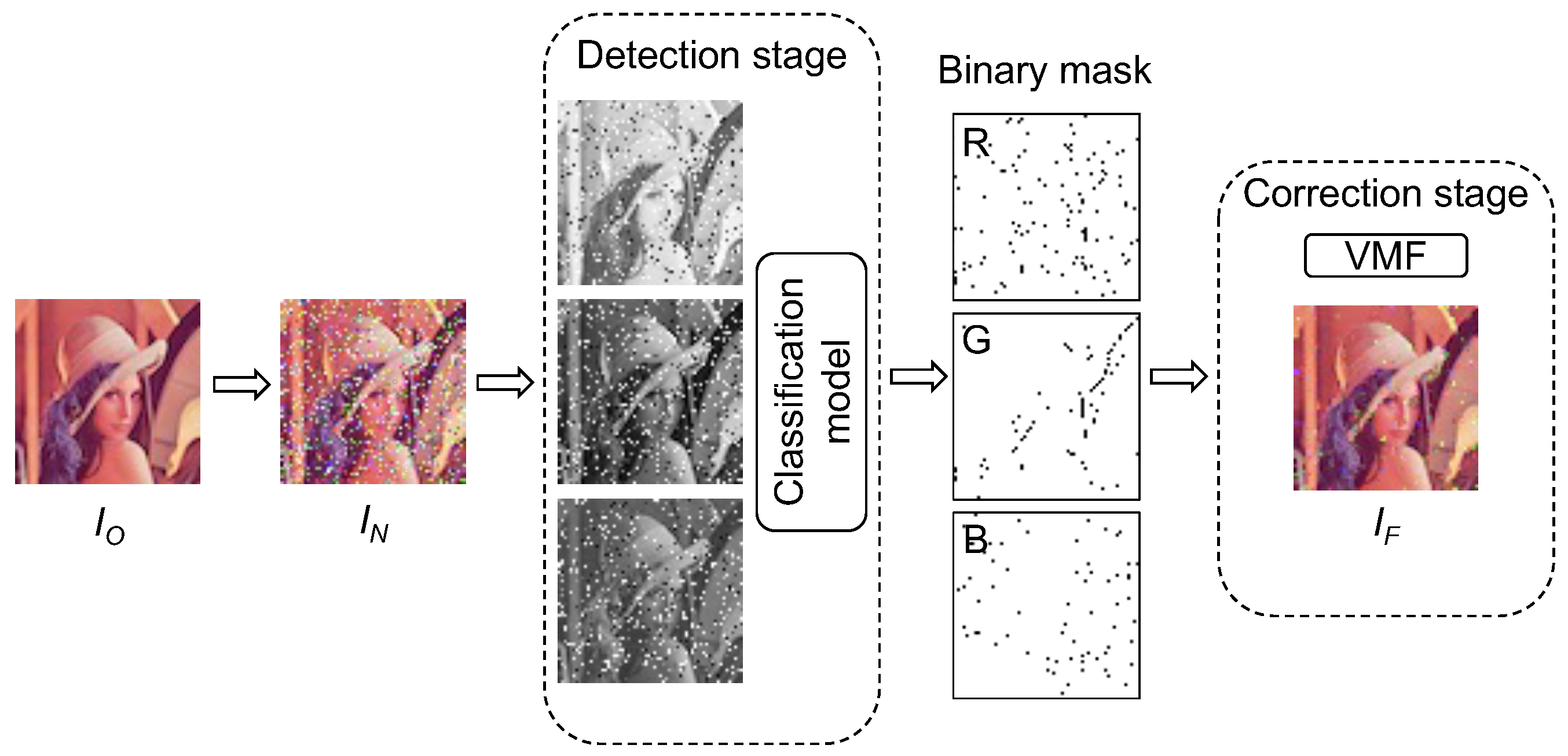
The proposed adaptive filter consists of two main stages for color image denoising: detection and correction. The detection stage takes a color image $I_N$ perturbed by impulse noise as input. In this stage, the color image is split into R, G, and B channels to separately evaluate each pixel in a binary classification model. For each channel, the model produces a binary mask representing the set of pixels classified as noisy.

The correction stage uses a version of a vector median filter applied only to the identified noisy pixels. The correction process of any pixel ${\overrightarrow{x}}_i$ consists of modifying one or more of its RGB channel values according to the pixel intensity values of its neighbors. In this context, the set of neighboring pixels of ${\overrightarrow{x}}_i$, denoted as $\mathcal{N}\left({\overrightarrow{x}}_i\right)$, represents a $3\times 3$ square window centered on ${\overrightarrow{x}}_i$ in the spatial domain of the image. Modifying the pixel value of ${\overrightarrow{x}}_i$ requires computing the sum of the absolute differences of the pixel intensities between ${\overrightarrow{x}}_i$ and its neighborhood. These differences among pixel intensities around ${\overrightarrow{x}}_i$ are denoted as $d_i^{\mathcal{N}\left({\overrightarrow{x}}_i\right)}$ such that

$$d_i^{\mathcal{N}\left({\overrightarrow{x}}_i\right)}=\sum _{\forall {\overrightarrow{x}}_j\in \mathcal{N}\left({\overrightarrow{x}}_i\right)}\left|\right|{\overrightarrow{x}}_i-{\overrightarrow{x}}_j{\left|\right|}_1.$$

(6)

Let $D\left({\overrightarrow{x}}_i\right)$ be the set of the pixel intensity differences between every pair of pixels considering ${\overrightarrow{x}}_i$ and its neighborhood, i.e., $D\left({\overrightarrow{x}}_i\right)=\left\{d_j^{\mathcal{N}\left({\overrightarrow{x}}_i\right)}\right|\forall {\overrightarrow{x}}_j\in \mathcal{N}\left({\overrightarrow{x}}_i\right)\}$. Then, a noisy pixel ${\overrightarrow{x}}_i$ is replaced (in one or more of its channels) with the element with the minimum values from $D\left({\overrightarrow{x}}_i\right)$. If only one channel of pixel ${\overrightarrow{x}}_i$ is identified as noisy (and the other two are not), only the perturbed value of this channel is replaced. On the other hand, if at least two channels are noisy in ${\overrightarrow{x}}_i$, then the pixel is replaced entirely. Since building the set $D\left({\overrightarrow{x}}_i\right)$ requires $O\left(1\right)$ time given a fixed $3\times 3$ window, the correction of the noisy pixels takes $O\left(N\right)$ time to complete. After the correction process, a new color image $I_F$ is generated. Figure 1 illustrates the two stages of the adaptive filter.

Figure 1. The sequence of the adaptive filter’s stages: the detection stage takes as input a noised image $I_N$, splitting it into its color channels, and then it uses a classification model to detect noisy pixels; the correction stage uses a vector median filter to repair only the detected noisy pixels.

4.1. Genetic Programming Design

We use genetic programming to generate the binary classification model for detecting noisy pixels in a color image. In a typical machine learning workflow, the training stage involves using a dataset to produce the classification model, whereas only a single image is required in the proposed evolutionary approach. This approach leverages the versatility and adaptability of the genetic programming design, allowing it to effectively learn and adapt to complex noise patterns using only a single training instance. This training image I has a noised version $I_N$ perturbed by the impulse noise models described in Section 3.1.

In this context, an individual is a classification model used to evaluate any pixel ${\overrightarrow{x}}_i$ of an image I to decide whether ${\overrightarrow{x}}_i$ is noisy. An individual is represented by a parse tree structure with $O\left(m\right)$ nodes selected from a set of primitives consisting of functions and terminals. The internal nodes of the tree consist of a set of functions $F=\{$add(x,y), sub(x,y), mul(x,y), mydiv(x,y), mysigmoid(x)}. Four elements of the set of functions denote the basic arithmetic operations of addition, subtraction, multiplication, and division. In particular, the division operator mydiv(x,y) is protected in the sense that it does not signal “division by zero”. The sigmoid function $\mathtt{mysigmoid}\left(\mathtt{x}\right)=\frac{1}{1+e^{-x}}$ guarantees that the results range between 0 and 1.

Additionally, the leaves of the tree consist of a set of terminals $T=\{$pc_dist, mu_dist, median_dist, sd_dist, pxc} that apply statistics operations to the set of neighboring pixels $\mathcal{N}\left({\overrightarrow{x}}_i\right)$ of pixel ${\overrightarrow{x}}_i$ in image I. Given a fixed $3\times 3$ window size, the computations of these statistics take $O\left(1\right)$ time. Table 1 describes the set of terminals. It should be noted that the selection of the set of primitives (functions and terminals) was mainly carried out through some preliminary experimental tests.

Table 1. Description of the set of terminal primitives T representing the different features of neighboring pixels.

Primitive	Description
pc_dist	The differences among pixel intensities around ${\overrightarrow{x}}_i$, i.e., $d_i^{\mathcal{N}\left({\overrightarrow{x}}_i\right)}$.
mu_dist	Average of the set $D\left({\overrightarrow{x}}_i\right)$.
median_dist	Median of the set $D\left({\overrightarrow{x}}_i\right)$.
sd_dist	Standard deviation of the set $D\left({\overrightarrow{x}}_i\right)$.
pxc	The RGB values of pixel ${\overrightarrow{x}}_i$.
$[-1\dots 1]$	Random values within the range of −1 to 1.

On the other hand, an individual’s fitness represents its ability to correctly detect noisy pixels in an image. For this aim, an image $I_O$ is perturbed using the three impulse noise models, each with a density of 10%, as described in Section 3.1. The produced noisy image $I_N$ is used as input for each individual of the initial population. Each individual of the population independently evaluates each pixel ${\overrightarrow{x}}_i$ of $I_N$ to decide whether ${\overrightarrow{x}}_i$ is perturbed by noise. Evaluating any pixel requires $O\left(m\right)$ time for any individual; therefore, the detection process requires $O\left(mN\right)$ time to complete. The output generated by each individual is a binary mask indicating which pixels are identified as noisy in $I_N$. This binary mask is used in the correction stage to produce the filtered image $I_F$, which is compared to $I_O$ via the image quality metrics PSNR and MAE described in Section 3.2. The results of these metrics are used to compute the individual’s fitness in the detection stage. It is worth noting that only these two metrics were chosen due to their low computational complexity. Figure 2 illustrates this procedure.

Figure 2. The fitness computation process for an individual $I_F$ of the population by comparing $I_F$ to an original reference image $I_O$.

4.2. The Proposed Evolutionary Algorithm

As part of the evolutionary process (also called training), the population of individuals produces offspring through crossover and mutation operators. The offspring have their fitness evaluated and compete for a place in the next generation. This process iterates until a certain number of generations is reached. This evolutionary process is described in Algorithm 1.    

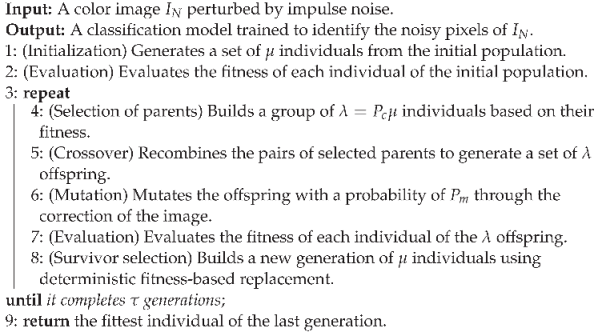
Algorithm 1: The evolutionary process of the detection stage

    Line 1 of Algorithm 1 generates an initial population of $\mu$ random individuals. To generate this population, we use the simplest and most popular full method to produce complete random trees. Each tree is generated recursively by randomly selecting primitives from the sets of functions and terminals. Primitives from the set of functions F are selected as the internal nodes of the tree, whereas those from the set of terminals T are selected as the leaves. The maximum depth of each of the initial trees is constrained to three. Considering random trees of size $O\left(m\right)$, the initial population generation requires $O\left(\mu m\right)$ time.

Lines 2 and 7 of Algorithm 1 perform the fitness evaluation of each individual of the population. The quality metrics MAE and PSNR, described in Section 3.2, are used for this aim. These metrics compare a filtered image $I_F$, produced by the detection and correction stages according to each individual, with its noiseless version $I_O$ (see Figure 2). The MAE indicates a better filter performance with a lower value, and the PSNR does the same with a higher value. Then, maximizing fitness is equivalent to maximizing the ratio between the MAE and PSNR. The fitness evaluation for all the $\mu$ individuals of the population takes $O\left(\mu mN\right)$ time. Note that the SSIM and FSIM are not considered in the fitness evaluation due to their higher computational complexity.

Line 4 of Algorithm 1 performs a random selection of pairs of individuals with replacement until it generates a group of $\lambda =P_c\mu$ individuals, where $P_c$ denotes the crossover ratio. The tournament selection is used to randomly select three individuals from the population and then select the fittest two. Implementing the tournament selection requires $O\left(\mu \right)$ time.

Line 5 of Algorithm 1 recombines pairs of individuals from the group selected by Line 4. A one-point crossover is used, where a random vertex is chosen within two copies of parent individuals, and then they exchange the subtrees rooted at the selected vertices between them. Recombining the entire population requires $O\left(\mu \right)$ time.

Line 6 of Algorithm 1 implements the uniform mutation operator to introduce diversity in the population. This operator takes as input an individual with probability $P_m$, and then it randomly selects a vertex of the tree to replace it with a new random subtree. Each subtree is generated using the full method in $O\left(m\right)$ time. Thus, uniform mutation applied to the $P_m\lambda$ offspring takes $O\left(\mu m\right)$ time.

Line 8 of Algorithm 1 generates a new population through the union of the $\mu$ individuals from the last population and their $\lambda$ offspring. A fitness-based replacement (implemented with a sorting algorithm) is used, guaranteeing the survival of the fittest individuals. The execution time of this step is $O(\mu log\mu )$.

Finally, Algorithm 1 iterates Lines 4–8 until they complete $\tau$ generations. Then, the algorithm returns the fittest individual of the last generation (Line 9). The overall execution time of Algorithm 1 is $O\left(\tau \mu \right(mN+log\mu \left)\right)$.

5. Experimental Results

Experiments were conducted to evaluate the performance of the proposed adaptive filter. The filter was implemented using scikit-image 0.18.3, a Python module that includes a collection of algorithms designed for image processing. Additionally, the evolutionary process (described in Algorithm 1) and its variation operations were implemented using DEAP 1.2.2, an open source evolutionary computation framework. The experiments were carried out on a 3.6 GHz Intel Core i7 (Mac) with four cores, 8 GB of RAM, and OS X 11.5.2.

5.1. Determination of Parameters

The classification model’s training process was performed using a 24-bit color version of the popular image of Lena. This training image, denoted as $I_N$ in Section 4, was simultaneously contaminated by the three impulse noise models with a total density of 30%, i.e., 10% for each of the models described in Section 3.1. Combining the impulse noise models into a single image provides insights into the algorithm’s ability to handle various noise types and densities by evaluating the proposed method’s robustness, generalization capabilities, and potential practical utility in image processing applications.

On the other hand, Table 2 shows the evolutionary settings used by the genetic program during the training process. These settings were estimated via experimentation and validation. A set of preliminary trials was conducted to find the best parameters of Algorithm 1 by considering the tradeoff between time and efficiency; however, similar to other evolutionary techniques, this approach has the limitations expressed in the NFL (no free lunch) by considering that there is no single set of evolutionary settings that will perform optimally on all possible color digital images.

Table 2. Configuration settings of the proposed genetic programming algorithm related to its behavior and performance during the training process.

Parameter	Value
Population size, $\mu$	100
Crossover rate, $P_c$	$0.9$
Mutation rate, $P_m$	$0.1$
Parent selection	Tournament ($k=3$)
Survivor selection	Fitness-based $(\mu +\lambda )$
Completion criteria	When the algorithm reaches $\tau =100$ generations

After model training, a set of trees (representing the individuals of the last generation) was produced. Each of these trees comprises the set of primitives (functions and terminals) described in Section 4.1. The tree identified as the fittest individual is available in a PDF, which can be downloaded from https://bitbucket.org/dfajardod/impulse_noise_gpfilter/src/ (accessed on 20 October 2023).

5.2. Benchmarks

Thirty benchmarking color images were used as test images for the proposed adaptive filter (GP). Each of these images was perturbed by the three impulse noise models with four different densities (5%, 10%, 15%, and 20%), i.e., a total of 360 test color images. These noise densities were selected to ensure a more equitable comparison among the different comparison filters. This decision stems from the recognition that certain filters have been specifically designed for higher noise densities, whereas others may perform more effectively in scenarios with lower noise levels. By evaluating the filters across an intersecting range of noise densities, we aim to conduct a comprehensive and balanced assessment. In this vein, the comparison of filters encompassed a diversity of robust and adaptive filters, some of which are widely used in digital image processing, whereas others use advanced adaptive methods. Filters using fuzzy logic tools to provide adaptiveness to local features were used, such as the fuzzy metric peer-group filter (FMPGF) and the noise adaptive fuzzy switching median (NASFM). Additionally, the decision-based algorithm for removing impulse noise (DBAIN) was also used, a filter designed for highly corrupted color images. Given their performance, the vector median filter (VMF) and the generalized synthesis and analysis prior algorithm (GSAPA) were also considered. Finally, a deep learning approach, the impulse detection convolutional neural network (IDCNN), was also used. The performance metrics used to compare the quality of the resulting images of these filters were the MAE, PSNR, SSIM, and FSIM (described in Section 3.2).

5.3. Performance of the Detection Stage

Experiments were conducted to measure the performance of the binary classification model implemented in the detection stage of the proposed GP filter. To this end, prior information about noisy pixel locations was stored by comparing the 360 test noisy images with their noiseless original counterparts. Later, the detection stage of the proposed GP was applied by classifying pixels as noisy or not noisy. Finally, a comparison of the model predictions with the stored prior information enabled the generation of a confusion matrix containing true positive (tp), true negative (tn), false positive (fp), and false negative (fn) predictions. The performance metrics applied to these predictions were the following: accuracy, precision, recall, specificity, and F1 score.

Accuracy (Acc.) indicates the extent to which the predictions about the condition of the pixels differed from the real conditions, i.e., Acc = (tp + tn)/(tp + tn + fp + fn). Precision (Prec.) indicates how well the classifier performed concerning each pixel’s noisy or noiseless status, computed by tp/(tp + fp). On the other hand, recall (or sensitivity) is the percentage of noisy pixels that were correctly identified, calculated by tp/(tp + fn). Similarly, regarding the noiseless pixels, specificity (Spec.) is calculated by tn/(tn + fp). Finally, the F1 score represents the harmonic mean of precision and recall, i.e., F1 = (Prec·Recall)/(Prec + Recall).

Table 3 shows the average results of the performance metrics regarding the proposed binary classification model. As can be observed, in general, the model increased the accuracy, precision, and F1 score according to the increase in the image’s noise density, whereas the sensibility and specificity decreased in this respect. Note that the model is highly efficient in detecting noisy rather than noiseless pixels. Finally, although the model achieved a better balance between precision and recall in terms of salt-and-pepper noise, better accuracy was obtained in terms of uniform and correlated noise.

Table 3. Average performance of the binary classification model applied to the test images perturbed by salt-and-pepper, uniform, or correlated noise.

		$\mathit{p}=0.05$	$\mathit{p}=0.10$	$\mathit{p}=0.15$	$\mathit{p}=0.20$
Salt and pepper	Acc.	0.7558	0.7462	0.7696	0.7906
	Prec.	0.3668	0.5107	0.6192	0.6963
	Recall	0.9981	0.9939	0.9853	0.9702
	Spec.	0.7191	0.6635	0.6495	0.6412
	F1	0.5306	0.6697	0.7570	0.8086
Uniform	Acc.	0.8217	0.7852	0.7776	0.7826
	Prec.	0.3559	0.4647	0.5479	0.6163
	Recall	0.9829	0.9796	0.9740	0.9667
	Spec.	0.8053	0.7427	0.7081	0.6890
	F1	0.5175	0.6271	0.6991	0.7514
Correlated	Acc.	0.8676	0.8428	0.8354	0.8409
	Prec.	0.3009	0.4139	0.4994	0.5773
	Recall	0.9948	0.9934	0.9909	0.9873
	Spec.	0.8611	0.8266	0.8088	0.8054
	F1	0.4515	0.5738	0.6547	0.7209

Since the correction stage of the proposed GP filter consists of a modified version of the VMF (see Section 4), the average performance comparisons shown in the following section allow us to determine the influence of the detection stage on the efficiency of the GP filter.

5.4. Performance of the Proposed Filter

Table 4 and Table 5 show the average results of the quality metrics obtained after filtering the test images to remove each of the impulse noise models: salt and pepper, uniform, and correlated. Table 4 presents the average values of the MAE and PSNR, whereas Table 5 shows those corresponding to the SSIM and FSIM.

Table 4. Performance comparison of the average MAE and PSNR values of the filters applied to the test images perturbed by salt-and-pepper, uniform, and correlated noise. The best, second-best, and third-best values are indicated in purple, teal, and brown, respectively.

	Filter	$\mathit{p}=0.05$		$\mathit{p}=0.10$		$\mathit{p}=0.15$		$\mathit{p}=0.20$
		MAE	PSNR	MAE	PSNR	MAE	PSNR	MAE	PSNR
Salt and pepper	IDCNN [33]	0.7903	38.1716	1.4747	34.4618	2.4699	29.4046	4.9519	23.0100
	GP	1.0939	35.0095	1.5978	31.5771	2.5213	27.6317	4.1993	23.6414
	DBAIN [25]	0.4772	38.4290	0.7630	36.0019	1.1004	34.0328	1.5002	32.3204
	NAFSM [22]	0.6070	36.1685	0.9462	34.2428	1.2883	32.9280	1.6345	31.8994
	GSAPA [17]	2.6156	31.7966	2.9833	31.0663	3.5351	30.1346	4.2661	29.2487
	FMPGF [20]	2.2195	28.8003	3.8605	24.0488	6.5878	20.4174	10.4068	17.8075
	VMF [16]	3.1961	30.5483	3.8062	27.4112	5.1515	23.2530	8.0343	19.2650
Uniform	IDCNN [33]	0.7684	38.3377	1.3842	35.3368	2.0003	33.3050	2.7118	31.1671
	GP	1.0140	34.4532	1.3874	32.1703	1.9043	30.1309	2.6113	28.2127
	DBAIN [25]	4.8939	20.3859	9.1438	17.5642	13.3550	15.8917	17.5735	14.6853
	NAFSM [22]	4.8221	20.4132	9.2765	17.5368	13.6620	15.8390	18.0242	14.6200
	GSAPA [17]	2.6536	31.7040	2.9988	31.0339	3.4723	30.2954	4.2545	29.2325
	FMPGF [20]	2.2267	29.4335	3.2508	27.5745	4.3313	26.0814	5.5097	24.7540
	VMF [16]	3.1275	31.6515	3.4545	30.3364	3.8811	28.9711	4.4963	27.3815
Correlated	IDCNN [33]	0.3695	42.2402	0.6119	39.4709	0.8544	37.7503	1.0627	36.6582
	GP	0.9586	34.9322	1.2799	32.9630	1.7195	30.9907	2.3007	29.0910
	DBAIN [25]	4.8995	20.3836	9.1560	17.5635	13.3640	15.8837	17.6076	14.6789
	NAFSM [22]	4.8599	20.3924	9.2837	17.5376	13.6712	15.8314	18.0630	14.6114
	GSAPA [17]	2.6684	31.6861	3.0830	30.9442	3.7525	29.8858	4.7601	28.4749
	FMPGF [20]	1.5161	31.8201	1.8178	31.0714	2.1347	30.3423	2.4708	29.6420
	VMF [16]	3.1635	31.5580	3.4802	30.3551	3.8537	29.1292	4.3345	27.7417

Table 5. Performance comparison of the average SSIM and FSIM values of the filters applied to the test images perturbed by salt-and-pepper, uniform, and correlated noise. The best, second-best, and third-best values are indicated in purple, teal, and brown, respectively.

	Filter	$\mathit{p}=0.05$		$\mathit{p}=0.10$		$\mathit{p}=0.15$		$\mathit{p}=0.20$
		SSIM	FSIM	SSIM	FSIM	SSIM	FSIM	SSIM	FSIM
Salt and pepper	IDCNN [33]	0.9902	0.9928	0.9788	0.9846	0.9461	0.9659	0.8297	0.9056
	GP	0.9792	0.9872	0.9681	0.9819	0.9365	0.9682	0.8642	0.9360
	DBAIN [25]	0.9919	0.9957	0.9875	0.9935	0.9819	0.9905	0.9745	0.9864
	NAFSM [22]	0.9888	0.9938	0.9828	0.9908	0.9770	0.9874	0.9712	0.9836
	GSAPA [17]	0.9681	0.9710	0.9610	0.9656	0.9476	0.9576	0.9256	0.9485
	FMPGF [20]	0.9475	0.9647	0.8679	0.9244	0.7452	0.8589	0.6209	0.7855
	VMF [16]	0.9472	0.9680	0.9146	0.9566	0.8162	0.9227	0.6514	0.8505
Uniform	IDCNN [33]	0.9907	0.9930	0.9829	0.9866	0.9729	0.9795	0.9537	0.9693
	GP	0.9748	0.9866	0.9609	0.9824	0.9371	0.9753	0.9010	0.9633
	DBAIN [25]	0.6042	0.8595	0.4702	0.7747	0.3899	0.7143	0.3318	0.6689
	NAFSM [22]	0.6036	0.8591	0.4693	0.7734	0.3888	0.7127	0.3307	0.6674
	GSAPA [17]	0.9672	0.9701	0.9602	0.9651	0.9478	0.9581	0.9195	0.9468
	FMPGF [20]	0.9305	0.9646	0.8891	0.9464	0.8493	0.9265	0.8108	0.9031
	VMF [16]	0.9519	0.9693	0.9413	0.9654	0.9219	0.9587	0.8857	0.9463
Correlated	IDCNN [33]	0.9951	0.9967	0.9923	0.9943	0.9894	0.9919	0.9868	0.9891
	GP	0.9780	0.9864	0.9706	0.9828	0.9563	0.9765	0.9313	0.9665
	DBAIN [25]	0.6352	0.8648	0.4885	0.7770	0.4017	0.7107	0.3399	0.6585
	NAFSM [22]	0.6348	0.8643	0.4876	0.7757	0.4007	0.7089	0.3386	0.6569
	GSAPA [17]	0.9663	0.9692	0.9545	0.9612	0.9278	0.9460	0.8818	0.9218
	FMPGF [20]	0.9728	0.9785	0.9680	0.9748	0.9628	0.9707	0.9572	0.9663
	VMF [16]	0.9533	0.9683	0.9446	0.9637	0.9313	0.9570	0.9080	0.9463

As observed in Table 4 and Table 5, in general, the proposed GP filter ranked second in average values across all quality metrics (MAE, PSNR, SSIM, and FSIM) for the uniform and correlated noise models, closely following the IDCNN filter. This suggests that the GP filter performed well overall compared to the other filters, particularly in conjunction with these noise models. Regarding salt-and-pepper noise, the DBAIN filter excelled across all quality metrics, closely paralleled by the NAFSM and IDCNN filters. This behavior was due to their specialization in detecting and removing this noise model. However, the competitiveness of the NAFSM and DBAIN filters declined for the uniform and correlated noise. Furthermore, the difference in magnitude of their average values for these noise models was significant, becoming more pronounced as the noise became more prevalent, showcasing a specialization that might not generalize well to other noise types. The IDCNN filter, based on a deep learning model, exhibited robustness to variations in the scale, orientation, and lighting conditions of color images, demonstrating its adaptability to different image textures and noise models. VMF, on the other hand, notably produced images with lower-quality values. This is because it did not differentiate between pixels based on their noise levels or the type of noise they exhibited, resulting in excessive blurring in images with large contrasting regions. Finally, the proposed GP filter generally outperformed the GSAPA and FMPGF filters across all noise models, demonstrating competitive performance across different noise models and ranking consistently well compared to other filters.

The average results presented in Table 4 and Table 5 encompass a diverse set of 360 test color images with different features such as size, shape, color texture, light conditions, edge characteristics, etc. The complete set of resulting filtered images, along with their original sizes and denoised versions, is available in the Supplementary Materials. However, four test images with different distinguishable characteristics were selected for illustrative purposes to visually analyze the filters’ efficiency: Baboon, Goldhill, Pepper, and Caps.

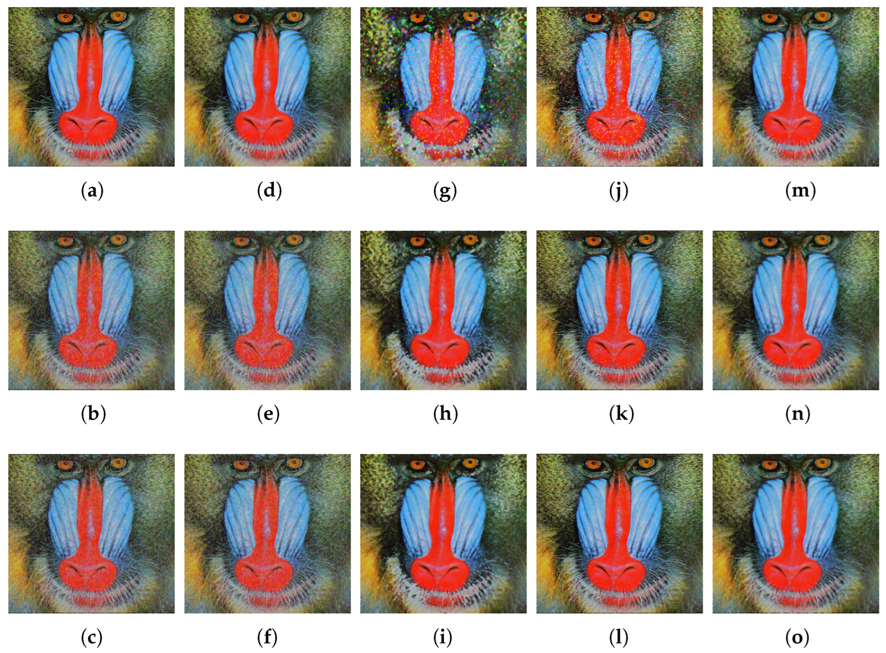
Figure 3 shows the visual results of some of the comparison filters applied to the Baboon image, considering the salt-and-pepper, uniform, and correlated noise models from top to bottom, respectively. Since the Baboon image has more profound and larger textured areas compared to the other test images, robust filters such as the VMF exhibited lower performance. Because of this, the resulting images of this filter were visually omitted. Among the filtered images, Figure 3a closely resembles the version of the image before adding noise. On the other hand, some filtered images show additional artifacts, e.g., Figure 3g. The ICDNN filter (Figure 3j–l) and the proposed GP filter (Figure 3m–o) excelled in noise removal while preserving the details of the images across the three different noise models.

Figure 3. Output images of the five best filters considering the Baboon image perturbed by salt-and-pepper, uniform, and correlated noise, with a noise density of $p=0.20$: (a–c) NAFSM; (d–f) DBAIN; (g–i) FMPGF; (j–l) IDCNN; (m–o) GP.

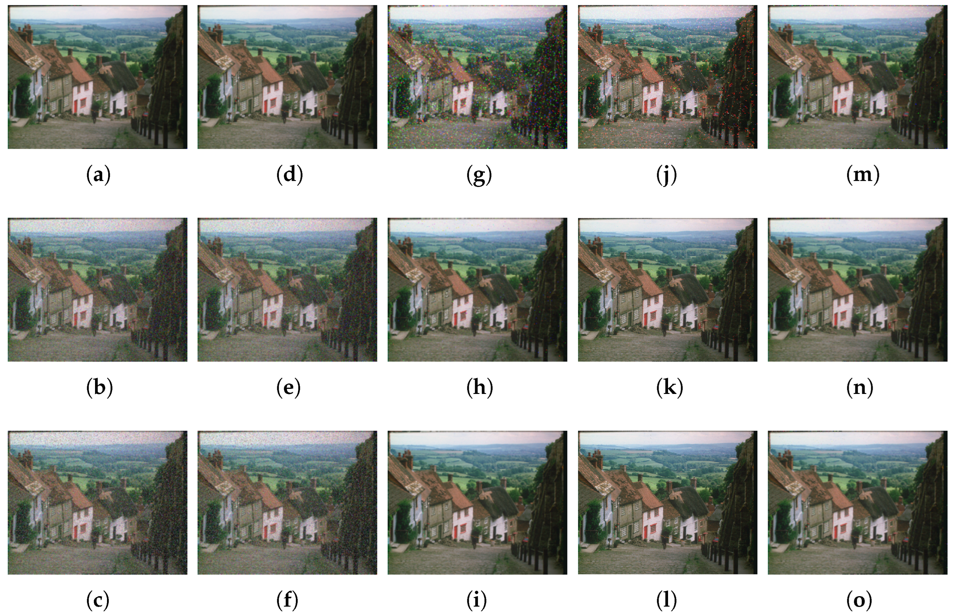
Figure 4 shows the resulting images produced by some of the comparison filters applied to the Goldhill image, arranged according to the three noise models from top to bottom. The Goldhill image has similar color tonalities to the Baboon image but has a few smooth areas and complex geometric patterns, resulting in significant contrast differences. For this reason, the filtered images shown here exhibit similar visual behavior to the filtered Baboon images. As observed in the filtered images, the NAFSM filter performed the best for salt-and-pepper noise (very close to the version of the image before adding noise). Although the IDCNN filter (Figure 4j–l) excelled in noise removal while preserving the details of the images for uniform and correlated noise, the proposed GP (Figure 4m–o) filter maintained consistent performance across the three different noise models. In general, the proposed GP filter ranked second for uniform noise and achieved some of the best MAE values for correlated noise.

Figure 4. Output images of the five best filters considering the Goldhill image perturbed by salt-and-pepper, uniform, and correlated noise, with a noise density of $p=0.20$: (a–c) NAFSM; (d–f) DBAIN; (g–i) FMPGF; (j–l) IDCNN; (m–o) GP.

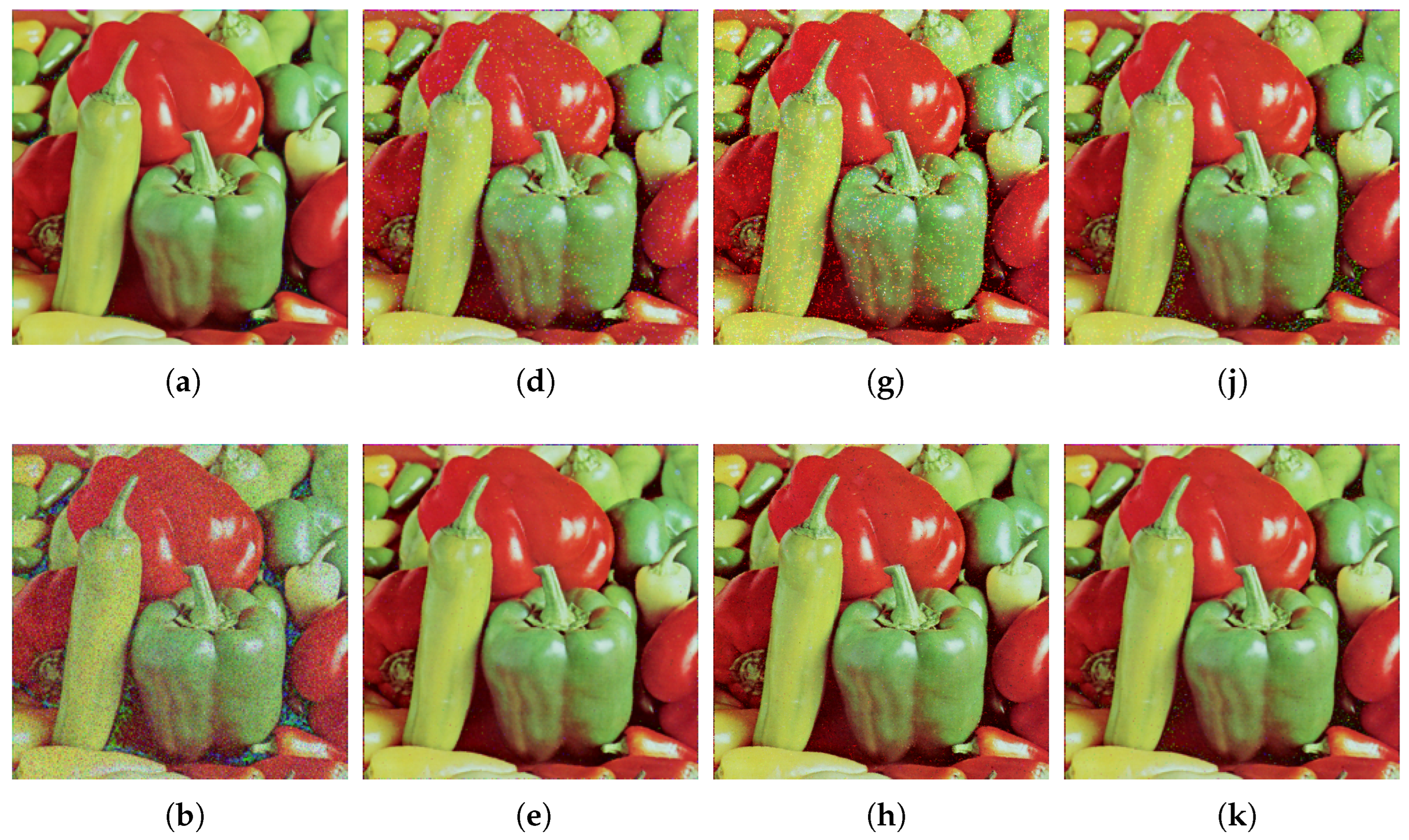
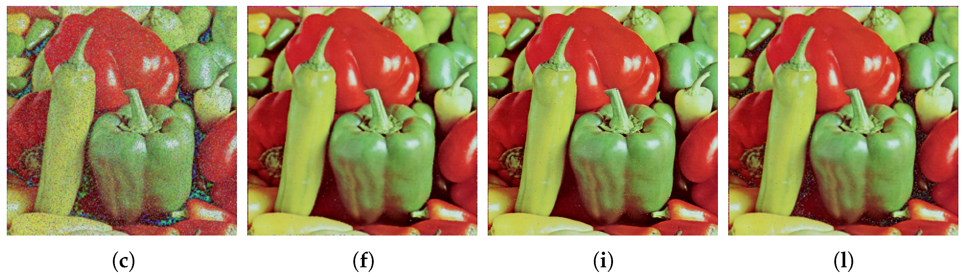
Figure 5 and Figure 6 show the filtered images produced by some of the filters applied to the images of the Peppers and Caps, respectively, including the VMF (which does not appear in Figure 3 and Figure 4). Unlike the previous images, in these images, the VMF demonstrates very competitive results across the three noise models, even producing some of the best images considering uniform and correlated noise. This is because these images have large, smooth regions with more contrast information. The VMF, IDCNN, and the proposed GP filters were generally competitive in these test images for both the uniform and correlated noise models.

Figure 5. Output images of the five best filters considering the Peppers image perturbed by salt-and-pepper, uniform, and correlated noise, with a noise density of $p=0.20$: (a–c) NAFSM; (d–f) VMF; (g–i) IDCNN; (j–l) GP.

Figure 6. Output images of the five best filters considering the Caps image perturbed by salt-and-pepper, uniform, and correlated noise, with a noise density of $p=0.20$: (a–c) NAFSM; (d–f) VMF; (g–i) IDCNN; (j–l) GP.

5.5. Discussion

In this context, overall performance relies on the capacity of a filter to simultaneously detect and remove any impulse noise model (salt and pepper, uniform, or correlated) without a preference or specialization. Therefore, the filtering process for each noise model can be seen as an objective function for a multi-objective problem. Each objective function depends on the image quality metrics used. Since a lower MAE value means fewer lost details in the image, searching for the optimum performance considering the MAE can be seen as a minimization multi-objective problem. Conversely, the cases for the PSNR, SSIM, and FSIM all represent maximization multi-objective problems (see Section 3.2). Figure 7, Figure 8, Figure 9 and Figure 10 illustrate the extent to which the performance of the comparison filters deviates with respect to a hypothetical optimum, also known as an equilibrium point in the context of multi-objective optimization [45]. In this work, the equilibrium point represents the best values obtained simultaneously for each corresponding noise model.

Figure 7. Three-dimensional Pareto front for MAE average values by considering the whole set of test images with noise densities $p=0.05, 0.10, 0.15$, and $0.20$.

Figure 8. Three-dimensional Pareto front for PSNR average values by considering the whole set of test images with noise densities $p=0.05, 0.10, 0.15$, and $0.20$.

Figure 9. Three-dimensional Pareto front for SSIM average values by considering the whole set of test images with noise densities $p=0.05, 0.10, 0.15$, and $0.20$.

Figure 10. Three-dimensional Pareto front for FSIM average values by considering the whole set of test images with noise densities $p=0.05, 0.10, 0.15$, and $0.20$.

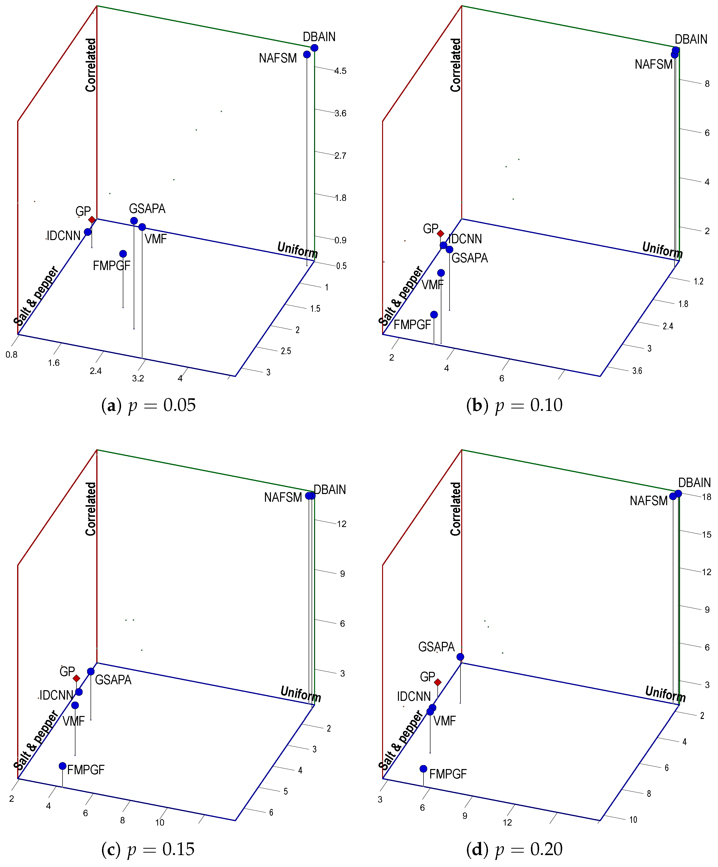
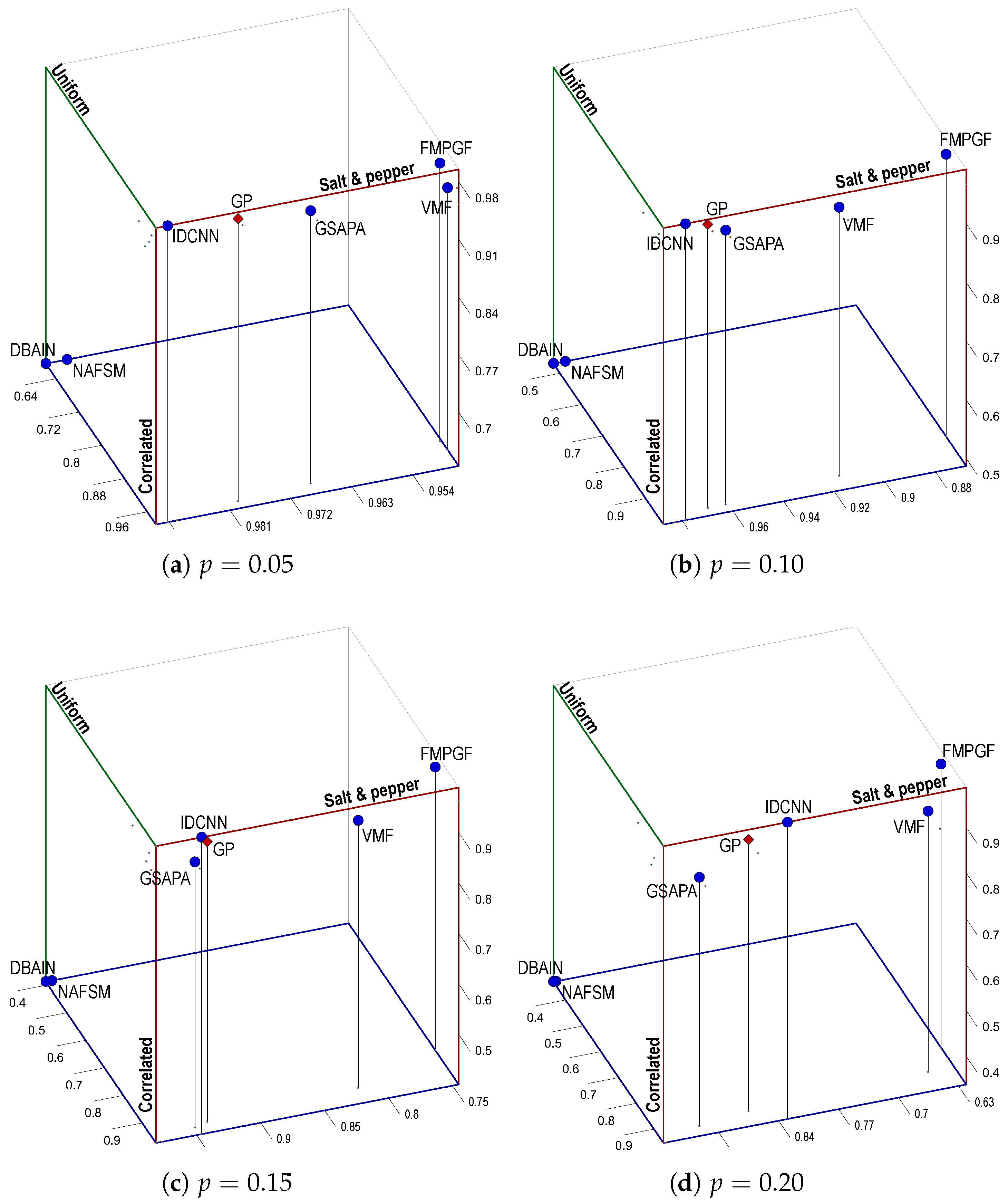
Figure 7 presents a three-dimensional Pareto front for the MAE average values, considering the complete set of test images with noise densities $p=0.05, 0.10, 0.15,$ and $0.20$. As can be observed, the MAE average values of the proposed GP filter (indicated by a red diamond) are among the closest to the equilibrium point for all noise densities, on par with the IDCNN and GSAPA filters. Given their specialization in salt-and-pepper noise, the NAFSM and DBAIN move away from the equilibrium point as the noise density level increases for the other two noise models. The average values of these two filters are located in a two-dimensional opposite extreme point at $p=0.20$. Consistent with the results of Table 4, the NAFSM and DBAIN are the furthest from the optimum.

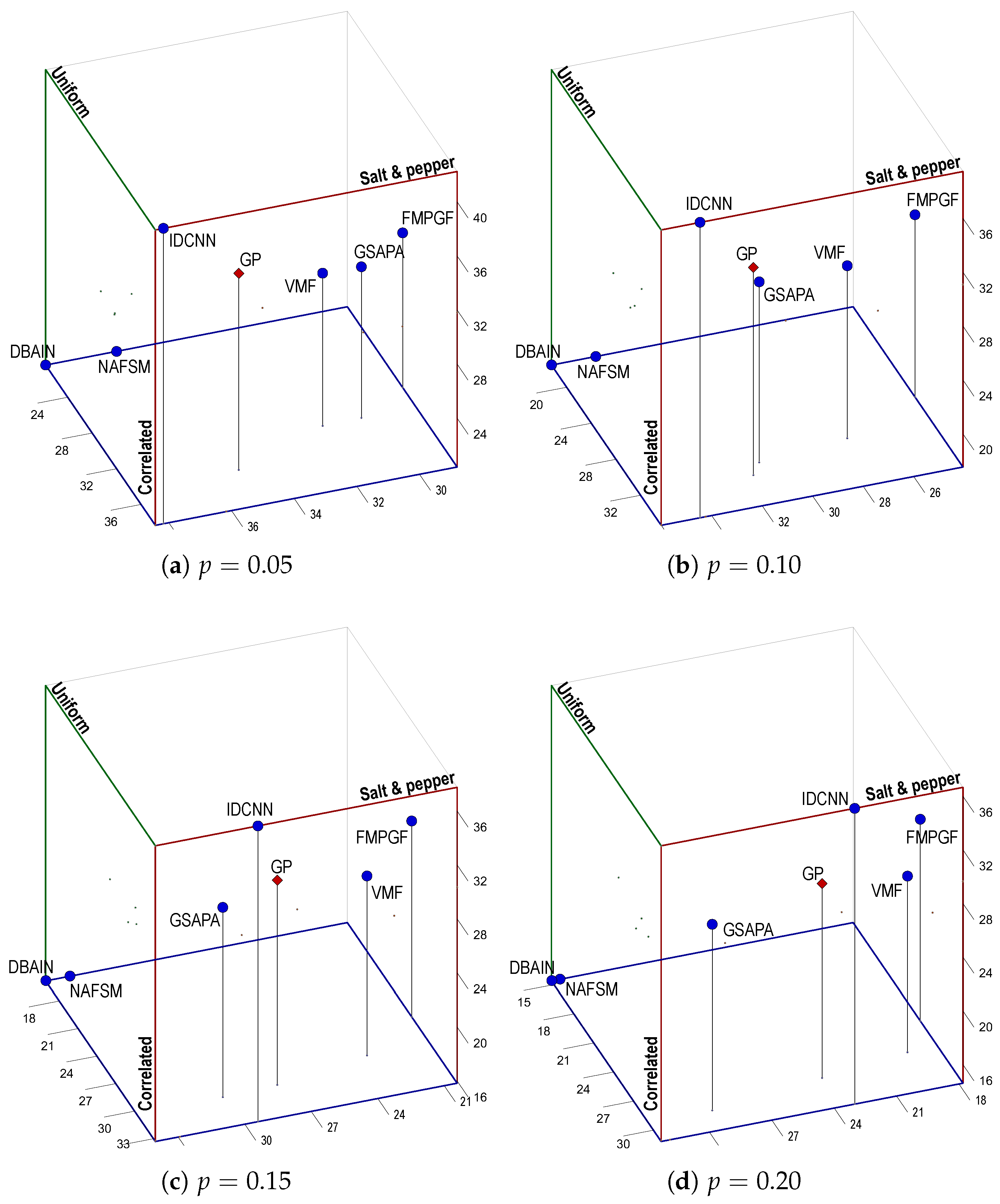
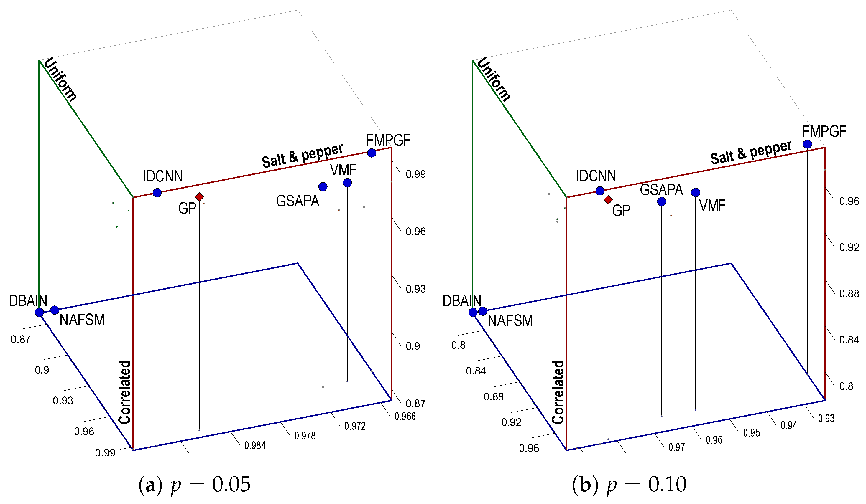
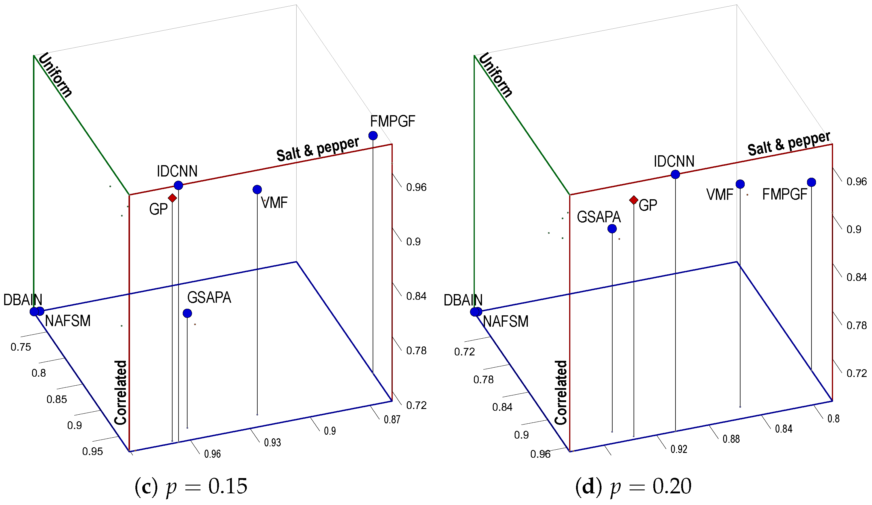
Similar to the behaviors shown in Figure 7 but oriented in the opposite direction, Figure 8 depicts the three-dimensional Pareto front for the PSNR average values. In this metric, the IDCNN filter demonstrates the best average values for the maximization multi-objective problem, followed by the GP filter, for $p=0.05$ and $0.10$. However, it is unclear which one of the average values of the IDCNN, GP, or GSAPA filters is the second closest to equilibrium for $p=0.15$ and $0.20$. It is also hard to determine which of the filters yields the furthest average values from the optimum. Unlike in Figure 7, the DBAIN is in a two-dimensional extreme point concerning the equilibrium point across all noise densities, followed by the NAFSM. Similarly to Figure 8, but with normalized values, Figure 9 and Figure 10 present the three-dimensional Pareto fronts for the SSIM and FSIM average values, respectively.

6. Conclusions and Future Work

This work presents an adaptive filter designed for the removal of three prevalent types of impulse noise, namely salt and pepper, uniform, and correlated noise, in color digital images. The proposed filter employs a two-step process, leveraging a binary classification model to identify noisy pixels within the image, followed by a correction step tailored to the specific color channels. What sets this proposed filter apart from the majority of filters utilizing classification models for noise removal is its high level of interpretability. This interpretability is a result of the evolutionary approach taken during model training—a process rooted in the principles of the genetic programming paradigm. By evolving the model through an iterative genetic programming framework, the resulting filter not only achieves effective noise reduction but also provides insights into the decision-making process of the classification model. Another distinctive feature of the training is that it only required a single image purposefully contaminated by the impulse noise models. Using a unique training image was particularly useful in reducing the computational complexity.

An experimental study was conducted to evaluate the performance of the proposed adaptive filter. A comparison with other filters was performed via the four image quality metrics (PSNR, MAE, SSIM, and FSIM). The experimental results show that most comparison filters present variability in the values of their quality metrics depending on the noise model and the image characteristics. In this vein, the proposed filter, called GP in Table 4 and Table 5, consistently obtained good performance values, second only to the ICDNN, which uses a deep learning-based approach. When measuring efficiency as a minimizing/maximizing multi-objective problem, as shown in Figure 7, Figure 8, Figure 9 and Figure 10, the proposed filter is one of the closest to an equilibrium point across all images and noise models used in the experiment, on par with the ICDNN and GSAPA filters.

Future work will focus on the integration of alternative machine learning techniques for the identification and correction of noisy pixels in color digital images. An intriguing avenue of exploration would be predicting the correlation of color channels to facilitate improved pixel replacement strategies within the image. This innovative approach holds promise for further enhancing the robustness and adaptability of the proposed adaptive filter in diverse real-world scenarios. It would also be interesting to explore how the genetic programming algorithm can be fine-tuned or adapted according to user preferences and specific requirements for noise removal in color images. Finally, optimizing the evolutionary settings of the genetic programming algorithm by employing other metaheuristic algorithms or ensemble approaches is also a topic left for future research.