Article

A Safe Admittance Boundary Algorithm for Rehabilitation Robot Based on Space Classification Model

1
School of Mechanical Engineering and Automation, Beihang University, Beijing 100191, China
2
Research Institute of Aero-Engine, Beihang University, Beijing 102206, China
*
Author to whom correspondence should be addressed.
Appl. Sci. 2023, 13(9), 5816; https://doi.org/10.3390/app13095816
Submission received: 24 March 2023 / Revised: 2 May 2023 / Accepted: 5 May 2023 / Published: 8 May 2023
(This article belongs to the Special Issue Surgical Robotics Design and Clinical Applications)

Abstract

:
Existing studies on rehabilitation robots are generally devoted to robot-assisted active rehabilitation training, which is conducive to facilitating muscle and nerve regeneration. However, human–robot interaction (HRI) requires imposing a limit on the workspace within which the robot operates, so as to ensure patient safety. A safe admittance boundary algorithm for a rehabilitation robot is proposed based on the space classification model which works by constructing a virtual boundary for the HRI workspace in the control layer. First, point cloud isodensification is performed for the workspaces within which the human body and the robot operate. Next, the nearest neighbor density is determined for the point cloud, and the space classification model is built on this basis. Finally, the space classification model is integrated with admittance control to derive the safe admittance boundary algorithm, which can be used for safety control. This algorithm is then subjected to space verification experiments and out–of–bounds experiments using a dynamic arm simulator (DAS). As indicated by the experimental results, when the side length of the voxel grid for voxel center filtering is set to 0.06 m, the accuracy of space definition is 98.40%. The average maximum response time for out–of–bounds behaviors is 165.62 ms. The safe admittance boundary algorithm can impose reasonable virtual constraints on the robot workspace, thereby improving HRI safety.

1. Introduction

The healthcare revolution in the second half of the 20th century has dramatically prolonged people’s life expectancies [1], although population aging has become a new social issue recently. Long-term healthcare services have to meet higher standards, given the prevalence of chronic disease in elderly people and the associated complications (e.g., cardiovascular disease and the resulting reduced muscle strength of the extremities, which leads to disabilities [2]). One major consequence is the sustainability risk faced by the healthcare system [3]. The significant shortage of rehabilitation nursing staff has already had some impact. Fortunately, rehabilitation robots have emerged as a new solution to this issue, along with the rapid progress in robot hardware and control technology.
Rehabilitation robots offer assistance in patients’ motor function recovery, guided by physical therapists [4,5]. They are usually designed for the purposes of therapeutic exercise, which helps in relearning and reactivating residual motor functions. Rehabilitation robots can also help prevent secondary complications such as muscular atrophy [6]. Earlier rehabilitation robots were originally designed for passive training to help patients in the acute stage [7]. However, passive training is not appropriate for all patients. In the non-acute stage, there is usually a greater need for the active training and recovery of motor flexibility and coordination of the limbs, which are highly important for muscle and nerve recovery [8,9]. So far, several human–robot collaborative controllers have been developed to support the active participation of users in rehabilitation. Typical controllers include force sensor-based impedance control [8,10], admittance control [11], assist-as-needed (AAN) control [12], minimal intervention control [13], and electromyogram-based compensation control [14].
However, safety issues in HRI are still not addressed for controllers and robots for active training purposes. Rehabilitation robots usually have heavyweight, high-power actuators and stiff joints and cooperate closely with patients in a shared workspace (HRI space) [15]. Additionally, patients are given greater control in active training when working together with robots. This means that if a robot does not fit with a patient, or there is a misoperation, the robot may move beyond the patient’s extremity range of motion, causing severe damage to the patient [16].
This problem has already been raised in earlier rehabilitation robot studies. During the development and optimization of the MIT-Manus wrist robot, Charles et al. designed a sliding mechanism to prevent joint mismatch [17]. Tejimad et al., inspired by the bio-reflection mechanism, designed a safe force sensor for faults to avoid a violation of space or collision in case the robot in the study went out of control [18]. Haraguchi et al. utilized ER fluid to add an ER brake and an ER actuator to the robotherapist in their study. These mechanisms could limit the robot’s range of motion by generating passive damping if dangerous robot motion was accidentally triggered [19]. Similar mechanisms developed elsewhere include magnetorheological (MR) clutches [20] and torque limiters [21].
Several new solutions have emerged in recent years due to continuous technological advances. Bae designed a driving mechanism with an electromagnetic sensor and an actuator to limit a robot’s field angle of motion so as to adapt to the safe range of motion of the human wrist [22]. Various methods have been described in literature [23,24] to limit the working ranges of robots by collecting physical (e.g., force and position) and psychophysiological (e.g., EMG and EEG) measurements to be integrated into their control strategies. Researchers in [25,26,27,28] took advantage of the low stiffness and the extensibility of flexible materials during the design of rehabilitation robots with the purpose of imposing flexible constraints on a robot’s range of motion.
Among various studies on the safety issues in HRI involving rehabilitation robots, some have optimized the robots to specifically reduce safety hazards. For example, a filter algorithm was designed and applied to cope with the accidental triggering of dangerous robot motions [16]. Alternatively, the possibility of secondary injury caused to patients can be reduced by optimizing the control strategy [29]. In another study, a safe strain diagram of muscles was built based on the biochemical model [30], and this was incorporated into the robot trajectory planning strategy to improve system safety. However, none of the described approaches can entirely circumvent the aforementioned safety hazards.
According to the literature review, a common solution to these hazards is to add a complex mechanism and sensors to the original equipment to limit the robot workspace. However, this will increase the complexity of the equipment and increase the costs, and this is not conducive to the use and popularization of rehabilitation robots [31]. In this paper, we propose a safe admittance boundary algorithm based on the space classification model for the force-sensing collaborative robots that have already been put into large-scale production. Virtual workspace constraints are imposed in the control layer (Figure 1) to elevate HRI safety in robot-assisted active training. First, the method for solving the workspace of the FK model is improved. The Monte Carlo method is combined with voxel center filtering to perform point cloud isodensification of the human and robot workspaces. Next, the nearest neighbor density is calculated in the point cloud. On this basis, a space classification model is built and integrated with admittance control. A variable stiffness admittance strategy is designed accordingly to construct the safe admittance boundary. Finally, the HRI safety is verified experimentally. In the simulation environment, the proposed algorithm is subjected to space verification experiments and out–of–bounds experiments using the dynamic arm simulator (DAS). The ability of the proposed algorithm to improve system safety is thus verified.
This paper presents three main contributions:
(1)
An algorithm model is proposed for identifying the safe space range based on the density of neighboring points in the point cloud.
(2)
The working space of the robot’s end degree of freedom is morphologically and reasonably restricted in the robot control layer.
(3)
This algorithm can improve the safety of HRI for collaborative robots in the field of upper limb rehabilitation.
The safe admittance boundary algorithm is described in four sections. Section 1 provides an overview of the algorithm. Section 2 introduces the point cloud isodensification of the workspace in the FK model. Section 3 describes the construction of the space classification model based on the nearest neighbor density in the point cloud. Section 4 presents the variable stiffness admittance strategy.

2. Safe Admittance Boundary Algorithm

2.1. Overview of the Algorithm

Figure 2 illustrates the overall flowchart of the safe admittance boundary algorithm. First, the Monte Carlo method and voxel center filtering are performed for the human and robot workspaces using the kinematic model. Two isodense point clouds with uniform point distribution in the space are obtained. Next, the nearest neighbor density is analyzed in the point cloud. The space classification model is built. The HRI space is determined. Finally, the variable stiffness admittance strategy is designed online based on the space classification model for admittance control. Thus, virtual constraints are imposed on the HRI space in the control layer by defining the safe admittance boundary.

2.2. Point Cloud Isodensification

To build the space classification model based on the distribution of point cloud densities, we perform point cloud isodensification in the human and robot workspaces. This results in two isodense point clouds with uniform distribution. Then, the method for determining the workspace in the FK model is improved by combining the Monte Carlo method and voxel center filtering. This method is illustrated in Figure 3.
First, the joint angle for each degree of freedom (DOF) is traversed under the two FK models using the Monte Carlo method. Specifically, random numbers are generated offline for the increment of the joint angle for each DOF using the Rand function under each of the two FK models. These random numbers are generated as many times as possible as depicted below:
g n , FK = g n , min + RAND × g n , max g n , min , n = 1 , 2 , 3 , , m
where g n , FK ,   g n , max ,   and   g n , min are the joint angle traversed in real-time for the n-th DOF and the upper and lower bounds of the joint angle for this DOF, respectively. m is the number of DOFs in the FK model. During the traversal of the joint angles for each DOF, 3D coordinates of the end-effector in the FK model are recorded. In this way, two point clouds representing the spaces accessible by the human arm and the robot are obtained.
Next, the side lengths of the minimum bounding box are calculated for each point cloud. The differences between the maxima X max , Y max , and Z max and minima X min , Y min , and Z min of the X-, Y-, and Z-axis values in the set of coordinates of the point cloud are calculated. On these bases, the side lengths l x ,   l y ,   and   l z of the minimum bounding box are estimated:
l x = X max X min l y = Y max Y min l z = Z max Z min
For the voxel octree representation, we build voxel grids for the first and second point clouds. Let the side length r of the voxel grids be equal between the first and second point clouds. That is, r 1 = r 2 , ensuring that the two point clouds that are outputted subsequently have the same density. For any point in the non-empty voxel, the voxel center C center x center , y center , z center is located based on the row, column, and lay of the voxel (row, col, lay) and the calculated minimal coordinates x min , y min , and z min for the voxel:
x center = x min + col 0.5 × r y center = y min + row 0.5 × r z center = z min + lay 0.5 × r
All non-empty voxels in the first and the second point clouds are traversed. Each voxel center approximately represents all other points in the same voxel. Finally, we obtain the first point cloud P i , FK 1 , i = 1 ,   2 ,   3 ,   , k FK 1 and the second point cloud P i , FK 2 , i = 1 ,   2 ,   3 , , k FK 2 with uniform point distribution. Here, k FK 1 = k FK 2 , where k FK 1   and   k FK 2 are the sizes of data of P i , FK 1 and P i , FK 2 , respectively.

2.3. Space Classification Model

With the isodensification of the two point clouds done, this section deals with the construction of a space classification model for HRI based on nearest neighbor density in the point cloud.
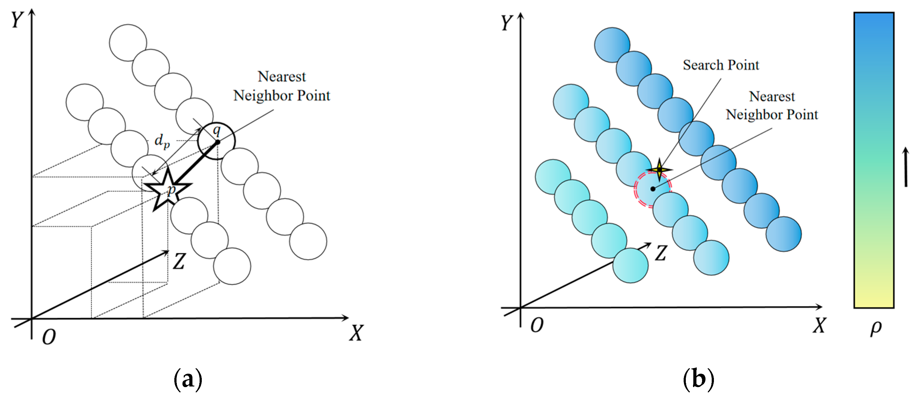
First, P i , FK 1 and P i , FK 2 are combined. The two sets of data points are represented in the same coordinate system based on the position and pose relationship between the human arm and the robot. The combined point cloud P i , combine , i = 1 ,   2 ,   3 ,   , k combine , is obtained and k combine is the size of data of P i , combine . Next, all points in P i , FK 1 , P i , FK 2 , and P i , combine are traversed. k-NN is used to search for the nearest neighbors of each point. The reciprocal of the Euclidean distance d p between each point and its nearest neighbor [32] is treated as the relative density ρ of the current point.
Specifically, P i , FK 1 , P i , FK 2 , and P i , combine are input as the training data set T for k-NN:
T = x 1 , y 1 , x 2 , y 2 , , x N , y N
where x i X 3 is the eigenvector of the data set: that is, the sample point Q . y i is the class of the data set, i = 1 ,   2 ,   3 , , N ; k = 1 is set for this model: that is, 1-NN nearest neighbor search. Hence, y i indicates that the class of x ’s nearest neighbor is the class of x. Meanwhile, the training data set is stored using a k-d tree for fast nearest neighbor search.
Any point p in the point cloud to be calculated is both the current point and the target point. q is any point other than p in the training data set T (as shown in Figure 4a). The Euclidean distance dis p , q is used to represent the distance between points p and q:
dis p , q = x p x q 2 + y p y q 2 + z p z q 2 2
Searching for the leaf node containing the target point p in the k-d tree involves the following steps. Start from the root node and recursively go down the k-d tree. If the coordinates of the target point in the current dimension are smaller than that of the splitting point, move to the left subnode; otherwise, move to the right subnode. Repeat the above process until the leaf node is reached. At this point, the leaf node is considered to be the current nearest neighbor.
Next, recursively move up the k-d tree. At each node, compare the Euclidean distance between the sample point stored in the data set and the target point and that between the current nearest neighbor and the target point. In the meantime, check whether there is a closer point near the other subnode with the same parent as the current subnode. Update the current nearest neighbor.
After returning to the root node, the last current nearest neighbor is the real nearest neighbor of the target point p in the training data set T.
Let d p be the minimum Euclidean distance between point p and other points in the point cloud (as shown in Figure 4a). The relative density ρ of the current point is given thus:
ρ = 1 d p = 1 min dis p , q , q = 1 ,   2 ,   3 , , N , p q
In the point cloud with uniform point distribution, d p is a fixed value. The relative density ρ of any point in the point cloud can be represented by a constant 1 d p ; the larger the value of d p , the smaller the relative density ρ of the point cloud, and the smaller the value of d p , the larger the relative density ρ of the point cloud.
To reduce the computational cost of the subsequent real-time operation, we calculate the relative densities of P i , FK 1 , P i , FK 2 , and P i , combine offline. All points in P i , FK 1 , P i , FK 2 , and P i , FK 2 are represented by the four-dimensional coordinates S x , y , z , ρ to obtain the four-dimensional point clouds P i , FK 1 , P i , FK 2 ,   and   P i , combine (as shown in Figure 4b).
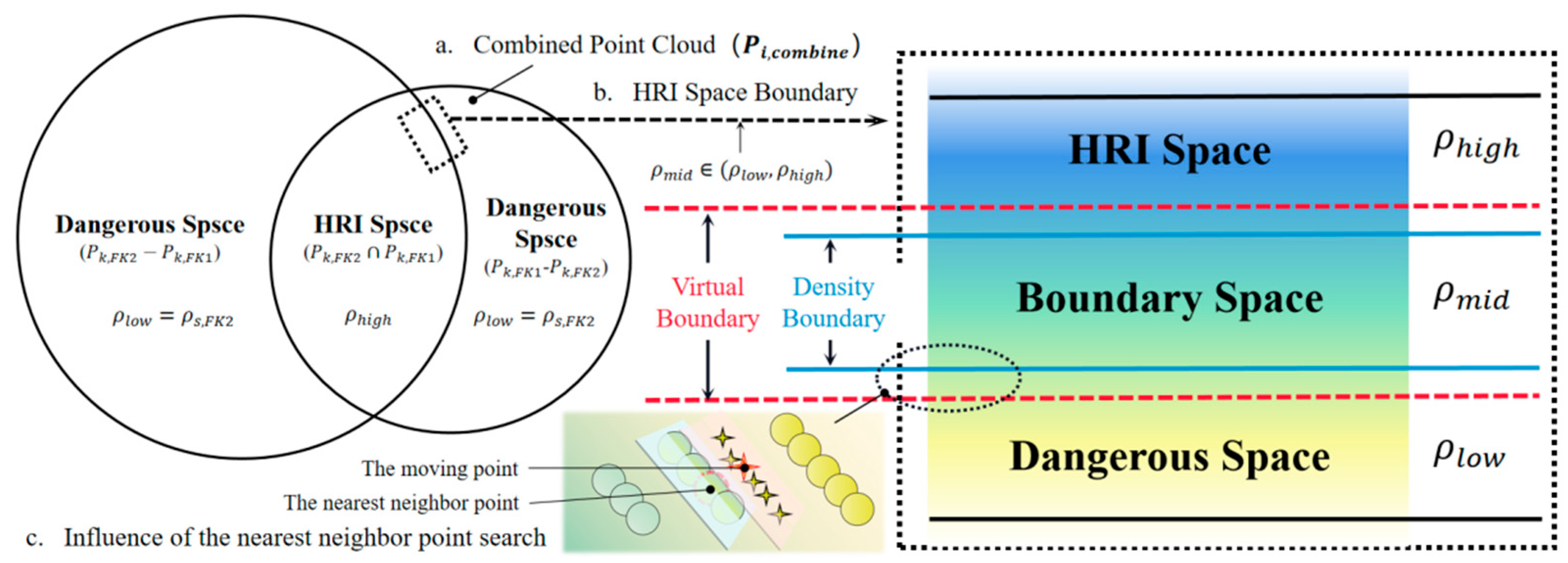
It can be observed that P i , FK 1 and P i , FK 1 have the same density at any point, which is a fixed value ρ low , i.e., ρ low = ρ s , FK 1 = ρ s , FK 2 . The maximal density is defined as ρ high in P i , combine . The density between ρ low and ρ high is represented by ρ mid , i.e., ρ mid   ρ low ,   ρ high .
Finally, the real-time moving point S   x   , y   , z   of the robot is introduced online into P i , combine as the target point. K-NN is used again to find the nearest neighbor for S   in P i , combine . The relative density ρ s , combine is calculated for this point. A comparison is made between ρ s , combine   vs .   ρ low   and   ρ high to build the space classification model. The algorithm is shown in Algorithm 1.
Algorithm 1 Space classification algorithm
1:
function Boundary judgment x d , y d , z d
2:
ω dan ←Dangerous Space, the dangerous workspace for HRI
3:
ω hri ←HRI Space, the safe workspace for HRI
4:
ω bou ←Boundary Space, the extreme workspace scope for HRI
5:
 (a) Load the moving point S ;
6:
 (b) Load P i , combine as the training data set;
7:
 (c) Search for the nearest point for S in P i , combine , according to the k-d tree structure and Equation (5);
8:
 (d) Obtain the density information ρ s , combine of the nearest neighbor point;
9:
 (e) Judge the space:
10:
  if ρ s , combine = ρ high then
11:
    return S d ω hri
12:
  else if ρ s , combine = ρ low then
13:
    return S d ω dan
14:
  else if ρ s , combine = ρ mid then
15:
    return S d ω bou
16:
  else
17:
    return False
Three woThree workspaces are defined for HRI in the algorithm. The density-defined spatial relationship between the three spaces is shown in Figure 5a. The space classification model is built based on the pattern of density variation of the point clouds (Figure 5b). Utilizing the influence of nearest neighbor search on the space boundaries (Figure 5c), we achieve the small-scale moving of the density-defined boundaries and the expansion of the workspaces. In this way, we delineate virtual boundaries with small-scale redundancy and build the space classification model.

2.4. Variable Stiffness Admittance Strategy

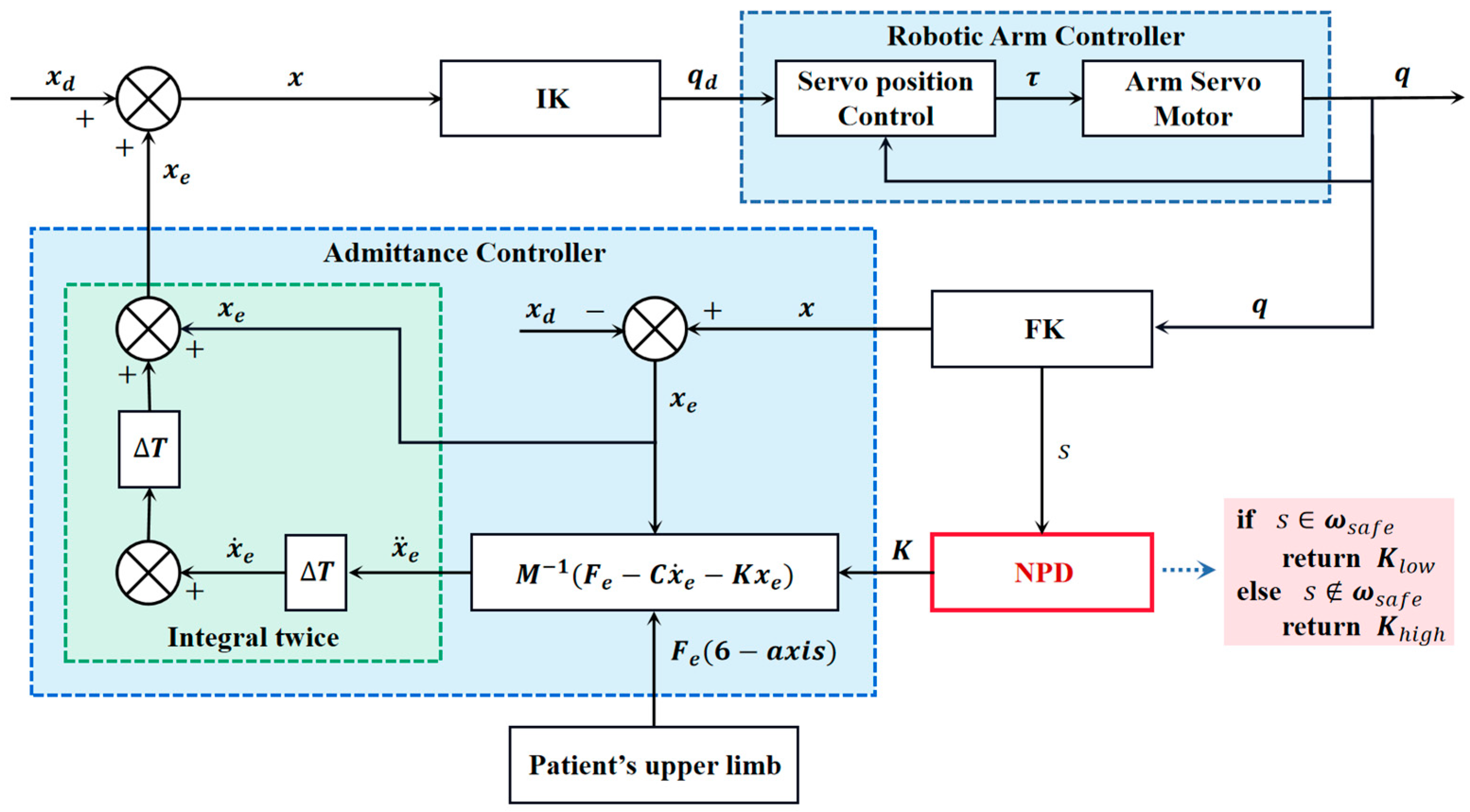
The space classification model is integrated with admittance control to impose virtual constraints on the workspace in the control layer. For this purpose, we design a variable stiffness admittance strategy to define the safe admittance boundary for the robot.
First, the real-time coordinates S   x   , y   , z   of the moving point in the end-effector of the robot are calculated using the admittance model and the position, pose, and six-dimensional force data of the end-effector. The admittance model is given below:
M x ¨ e + B x ˙ e + Kx e = F e
where: F e 6 is the force imposed by the human wrist on the force sensor; M 6 × 6 , B 6 × 6 , and K 6 × 6 are the virtual mass, virtual damping, and virtual stiffness in the admittance model, respectively;   x e 6 is the corrected position and pose; and x ˙ e 6 and x ¨ e 6 are the first- and second-order derivatives of   x e , respectively—that is, the velocity and acceleration of the corrected position and pose, respectively. The corrected position and pose x e = x x d = Δ v ,   Δ ξ . The corrected position and pose is the difference between the actual position and pose x   and the expected position and pose x d ; Δ v is the position deviation and Δ ξ is the pose deviation.
In the actual admittance model, we not only take into account the robot’s virtual mass M r 6 × 6 , virtual damping B r 6 × 6 , and virtual stiffness K r 6 × 6 , but also consider human dynamics [10]. We consider the human dynamics compensation, introduce human virtual mass compensation M h 6 × 6 , virtual damping compensation B h 6 × 6 and virtual stiffness compensation K h 6 × 6 in the admittance model, and define M = M r + M h , B = B r + B h , and K = K r + K h for the admittance model in this system.
In the process of HRI, the size of K has a direct bearing on the robot’s ability to track the intention of a human arm motion. A lower K value allows the patient to move in a greater range; a higher K value allows the robotic arm to more precisely track the expected position and pose or the motion trajectory. For the purpose of robot-assisted active training, a lower virtual stiffness K low is set for the initial admittance model of the robotic arm.
The acceleration of the corrected position and pose is calculated using the admittance model:
x ¨ e = M 1 F e B x ˙ e Kx e
Based on the acceleration of the corrected position and pose, the corrected position and pose is calculated by taking the quadratic integral:
X e = x ¨ e dt dt
The position and pose x   = x d +   x e of the moving point in the end-effector for the next moment is calculated based on the corrected position and pose and the expected position and pose input from robot motion planning. Inverse kinematics is implemented to determine the expected joint coordinate matrix q d for each joint to achieve robot motion control. The control gains are tuned by referencing [33]. Additionally, FK is applied to the real-time joint coordinate q   of the robot to obtain the real-time coordinate S   x   , y   , z   of the moving point in the end-effector.
Next, the boundary model of the HRI space is integrated with the admittance model. The architecture of the control layer of the variable stiffness admittance strategy is shown in Figure 6. Thus, we establish the variable stiffness admittance strategy (Algorithm 2). If S is located in the HRI space, the admittance model maintains a low stiffness K low . If S falls within the boundary space, an intermediate stiffness K mid is assigned to the admittance model. As a result, the moving point in the end-effector is more aligned with the expected position and pose x   or the expected motion trajectory as the stiffness increases. If S falls within the dangerous space, a higher stiffness K mid is assigned to the admittance model so that the robot can soon get back to the HRI space.
Algorithm 2 Variable stiffness admittance strategy algorithm
1:
function Variable Stiffness x   , y   , z  
2:
for all coordinates S ω rob do
3:
  if S ω safe then
4:
   return K low
5:
  else if S ω dan then
6:
   return K high
7:
  else if S ω tra then
8:
   return K mid
9:
  else
10:
    return False

3. Experiments

This section introduces the experimental protocol, experimental platform, and the human arm model used in our study. The DAS mentioned earlier is used for the space verification experiments and out–of–bounds experiments with the purpose of verifying the effectiveness and feasibility of the proposed algorithm.

3.1. Experimental Settings

The experimental workflow is shown in Figure 7. Experiments are conducted in two steps. These include space verification experiments and out–of–bounds simulation experiments.

3.1.1. Space Verification Experimental Settings

For the space verification experiments, DAS, developed using OpenSim—an open source software system for biomechanical modeling [34]—and Matlab software are used to construct the human upper kinematic model [35]. The musculoskeletal model involved in this simulator was built by Blana et al. in SIMM [36]. The anatomical data came from the cadaveric study conducted by Klein-Breteler et al. [37]
The test logic behind the experiments is shown in Figure 8. Two performance indicators, namely average judgment time and accuracy, are used to verify the effectiveness and feasibility of the proposed space classification model for determining the HRI space. Since the kinematic model of DAS is already known, the problem of judging the boundary of the HRI space is equivalent to that of defining the range of the collaborative space of the two robotic arms. We experimentally verified the accuracy of the space classification model using inverse kinematics. In the space verification experiments, 500 moving points are tested in total. The side length of the voxel grid for voxel center filtering is treated as an independent variable. We further determined the influence of the number of midpoints in the point clouds on the algorithm’s performance.

3.1.2. Out–of–Bounds Simulation Experimental Settings

In the out–of–bounds simulation experiments, three performance indicators are involved, namely the response time of the admittance model, trajectory of the moving point in the end–effector, and response time for out-of-bounds behaviors. The proposed safe admittance boundary algorithm is used to impose virtual constraints on the robot workspace to effectively and feasibly improve the HRI safety.
HRI safety testing is part of the experiment. A non-powered linkage mechanism with 4 DOFs and low damping and a six–dimensional force sensor (Force Torque Sensor, FT–300, Canada ROBOTIQ, Lévis, QC, Canada) are used to simulate the robot admittance model with low damping and no stiffness. Twenty groups of output force data of the wrist are collected from five experimenters during the active control of the motion of the shoulder and elbow. The space accessible by the five experimenters is measured. Compared with the space accessible by the upper arm in DAS, the former is larger. Therefore, the ability of the system to make an effective response when the moving point in the end–effector touches the safe admittance boundary could be reliably verified by the experiments.
For each collection, the subject’s wrist is attached to the six–dimensional force sensor by the hook and loop fasteners (as shown in Figure 9a). The subjects are asked to actively control the motion of the shoulder and elbow, with the upper arm making a linear reciprocating motion along the x–axis. The admittance model is configured based on the damping factor and stiffness coefficient of the linkage mechanism. The collected data are imported into the robotic simulation system (as shown in Figure 9b) for motion simulation and analysis.
The computer hardware for building the simulation system consists of the following components: Windows 10 operating system, Intel CPU i5–12400F, NVIDIA GPU RTX 3060, and 64 GB random access memory. The software environment consists of Matlab 2022b and Simulink 2022b. The side length r 1 = r 2 = 0.06   m of the voxel grid for voxel center filtering is configured in the experiment so that the response time of the variable stiffness admittance strategy is ensured. The sampling rate is set to 20 ms for the safe admittance boundary in the simulation, and K low is 0 N/m. The values of these parameters ensures that the response time requirements are met during rehabilitation training and that the motion features of the linkage mechanism used for data collection are fully considered. In the admittance model, M is set to 0.01 kg, B to 1 Ns/m, K mid to 5 N/m, and K high to 10 N/m. The expected position, a fixed point, lies at the center of the safe space.

3.2. Results

3.2.1. Space Verification Experiments

The point cloud for the space accessible by the human arm (Figure 10b) and by the robot is determined using DAS (Figure 10a) and the kinematic model with isodensification (Figure 10c). The four-dimensional combined point cloud is obtained using the space classification model (Figure 10d).
Forward kinematics is used for the traversal and simulated generation of 5000 real-time moving points of the robot. Three spaces involved in HRI are defined using the space classification model. Figure 11a shows the dangerous space, (b) the boundary space, and (c) the HRI space.
Based on the above, the side lengths r 1 = r 2 of the voxel grid for voxel center filtering are set to 0.02 m, 0.04 m, and 0.06 m, respectively, as shown in Table 1. The average judgment time is calculated for each, and the accuracy of each group of space classification experiments is verified by numerical inverse kinematics. The experimental results show that the maximum average judgment time is 11.6 ms and the lowest accuracy is 98.40%. Thus, the effectiveness and feasibility of the proposed method for defining the virtual boundaries based on HRI space analysis are demonstrated.
Meanwhile, it is found that the side length of the voxel grid influences the number of midpoints of the point cloud. Moreover, due to the influence of the space classification model on the boundary, the smaller the side length of the voxel grid was, the greater was the number of midpoints of the point cloud and the longer was the average judgment time. Nevertheless, the accuracy is higher in this case. In other words, the boundary and the space are more accurately represented.

3.2.2. Out–of–Bounds Simulation Experiments

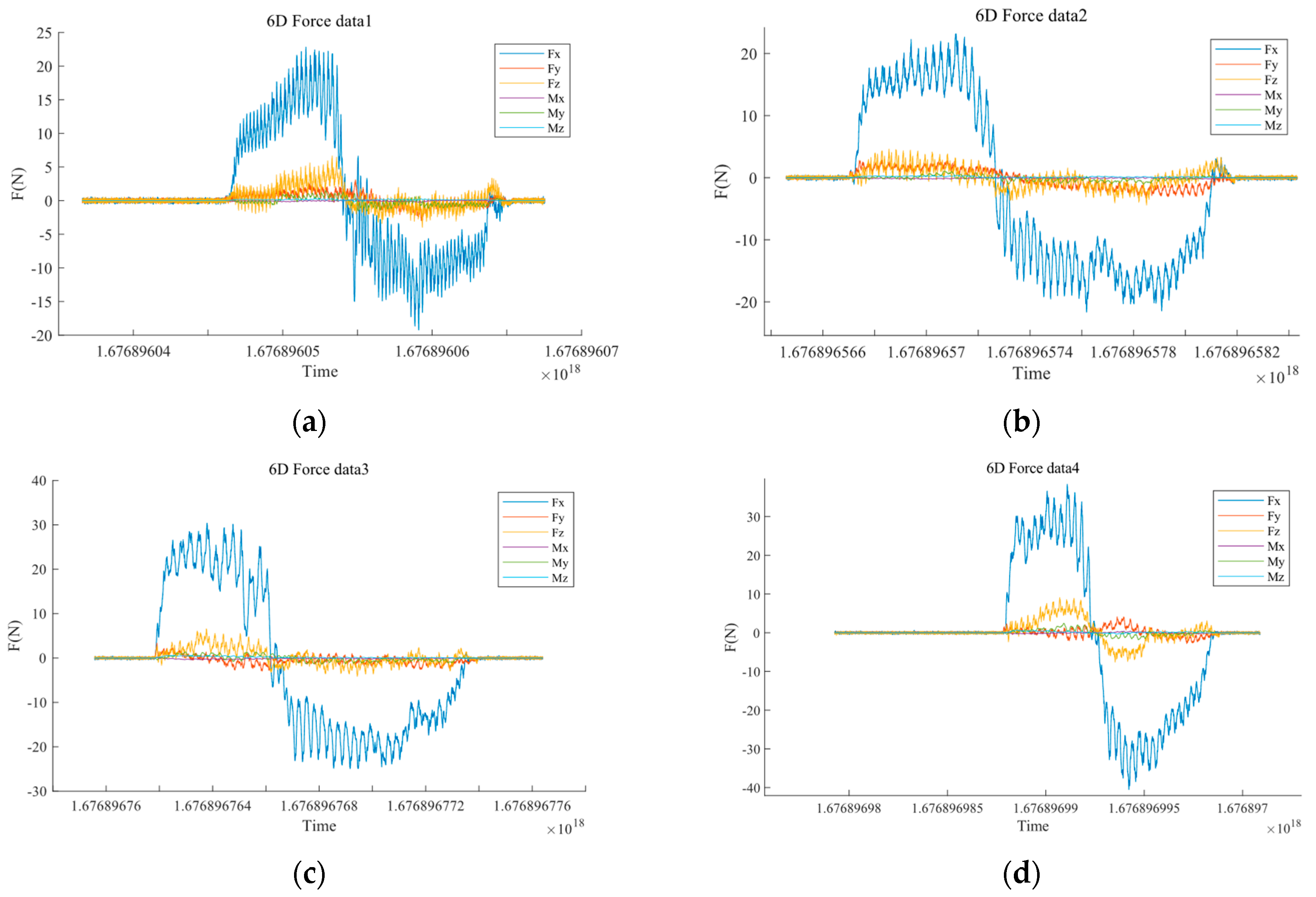
For the purpose of evaluation, the output wrist force data collected from the five experimenters with the same intended trajectory of motion are imported into the simulation system. Depicted in Figure 12a–d are the output forces of wrists from experiment, 1 making four groups of reciprocating motion in the same direction.
Figure 13a shows a small segment of the variation curve of the six-dimensional force FX after interception and filtering when experimenter 1 makes a motion along the specified intended trajectory. With this group of force data imported into the simulation system, the virtual mass m in the admittance model is consistently set to 0.01 kg and the virtual damping C is 1 Ns/m. The virtual stiffness k varies, its values being 0 N/m, 1 N/m, and 10 N/m, respectively. The velocity response curve output from the admittance model is obtained (as shown in Figure 13b).
When the virtual stiffness is 0 N/m, the velocity response curve in the admittance model shows a variation trend consistent with that of the input interactive force. As the interactive force increases, the velocity of robotic motion increases as well. This indicates that the admittance controller can effectively recognize and track human motion intention. When the virtual stiffness increases from 0 N/m, the variation trend of the velocity response is not consistent with that of the input force anymore. This means that the admittance controller loses the ability to track human motion intention. The end-effector moves at an expected velocity and tends towards the expected position and pose. The above results demonstrate the effectiveness of the variable stiffness admittance strategy in defining the safe admittance boundary.
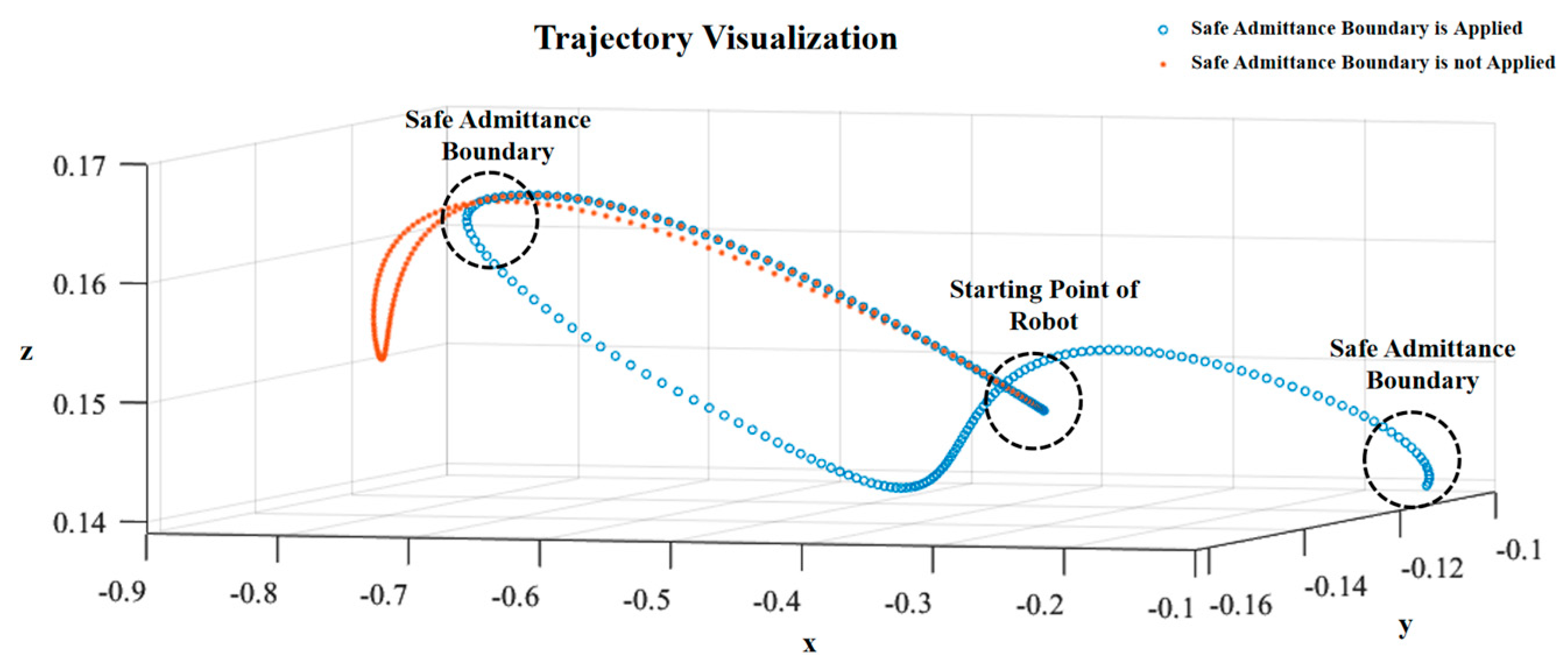
Figure 14 shows the trajectories of the moving point in the end-effector with the input of the same six-dimensional force data with and without the application of the safe admittance boundary in the robotic simulation system. Along the trajectory from the starting point to the safe admittance boundary, the trajectories of the end-effector output from the simulation system with and without the application of the safe admittance boundary completely overlap. The above results indicate that in the control layer, the safe admittance boundary is generally accurate in judging the scope of the moving point. Twenty groups of data are analyzed in the same manner, and similar findings are made. The simulation system with the application of the safe admittance boundary also executes a change in the trajectory of the moving point in the end-effector at the safe admittance boundary so that the robotic motion is confined within the safe admittance boundary. This result proves the effectiveness of the applied safe admittance boundary.
Finally, 20 groups of six–dimensional force data collected from the five experimenters are analyzed, as shown in Table 2. The above data are input into the simulation system. The average maximum response time for out-of-bounds behaviors is 165.62 ms. The kinesthetic reaction time of individuals without any known impairments typically falls within the range of 129.4 to 160.3 ms [38], and so the delay is almost imperceptible to the user. It is well demonstrated that the safe admittance boundary is timely and effective in recognizing and correcting out–of–bounds behaviors. In short, the safe admittance boundary is effective and feasible in ensuring HRI safety.

4. Conclusions

In this paper, a morphological model construction method of HRI workspace is proposed and a safety detection control algorithm is constructed by integrating the variable stiffness admittance strategy. Finally, the safe admittance boundary of the rehabilitation robot HRI process is established. Space verification experiments and out–of–bounds simulation experiments are conducted in the simulation system using DAS. As indicated by the experimental results, when the side length of the voxel grid for voxel center filtering is set to 0.06 m, the accuracy of the space definition is 98.40%. The average maximum response time for out-of-bounds behaviors is 165.62 ms. These experiments verify the accuracy of the virtual constraints imposed on the HRI space and the feasibility of this method in improving the HRI safety in robot-assisted training.
Our research lays the groundwork for using mass-produced, low-cost collaborative robots to provide safe physiotherapy for patients. However, before the proposed algorithm is put into practice, some limitations must be overcome. One is the scientificity of the kinematic model of the human upper arm. The introduction of DAS can improve the scientificity and accuracy of determining the space accessible by the upper arm using the proposed algorithm. However, a key issue affecting the definition of the safe admittance boundary is the question of how to more correctly determine the space accessible by the upper arms of different patients. The second is concerned with the application of collaborative robots in upper arm rehabilitation in real-world settings. We have already made efforts to avoid safety hazards caused by mismatches between robots and patients or misoperation of robots during active rehabilitation training. However, the collaborative robot needs to be empowered as a mediator for the scenario of active rehabilitation training. In the future, we will improve on the method for determining the space accessible by the upper arms based on clinical investigations. Forward kinematics of the human musculoskeletal system may be employed for robotic motion planning so that the robot can become a qualified mediator to offer professional and scientific rehabilitation guidance for patients. We will further verify the possibilities of using collaborative robots in assisting active rehabilitation training.

Author Contributions

Conceptualization, Y.T. and Y.J.; methodology, Y.T. and Y.J.; software, Y.J. and D.H.; validation, Y.J. and H.G.; formal analysis, D.H.; investigation, Y.J. and D.H.; resources, H.G.; data curation, H.G.; writing-original draft preparation, Y.J. and D.H.; writing-review and editing, Y.T. and T.W.; visualization, Y.J.; supervision, H.G.; project administration, Y.T. and T.W.; All authors have read and agreed to the published version of the manuscript.

Funding

This research was funded by the Sichuan Science and Technology Planning Project. Grant number: 2021YFSY003.

Institutional Review Board Statement

Not applicable.

Informed Consent Statement

Not applicable.

Data Availability Statement

Not applicable.

Conflicts of Interest

The authors declare no conflict of interest.

References

  1. Beach, B. Ageing Populations and changing worlds of work. Maturitas 2014, 78, 241–242. [Google Scholar] [CrossRef] [PubMed]
  2. Heiland, E.G.; Welmer, A.-K.; Wang, R.; Santoni, G.; Fratiglioni, L.; Qiu, C. Cardiovascular Risk Factors and the Risk of Disability in Older Adults: Variation by Age and Functional Status. J. Am. Med. Dir. Assoc. 2019, 20, 208–212.e203. [Google Scholar] [CrossRef] [PubMed]
  3. Lopreite, M.; Zhu, Z. The effects of ageing population on health expenditure and economic growth in China: A Bayesian-VAR approach. Soc. Sci. Med. 2020, 265, 113513. [Google Scholar] [CrossRef] [PubMed]
  4. Krebs, H.I.; Ferraro, M.; Buerger, S.P.; Newbery, M.J.; Makiyama, A.; Sandmann, M.; Lynch, D.; Volpe, B.T.; Hogan, N. Rehabilitation robotics: Pilot trial of a spatial extension for MIT-Manus. J. NeuroEng. Rehabil. 2004, 1, 5. [Google Scholar] [CrossRef]
  5. Mohammadi, E.; Zohoor, H.; Khadem, S.M. Design and prototype of an active assistive exoskeletal robot for rehabilitation of elbow and wrist. Sci. Iran. 2016, 23, 998–1005. [Google Scholar] [CrossRef]
  6. Centonze, D.; Koch, G.; Versace, V.; Mori, F.; Rossi, S.; Brusa, L.; Grossi, K.; Torelli, F.; Prosperetti, C.; Cervellino, A.; et al. Repetitive transcranial magnetic stimulation of the motor cortex ameliorates spasticity in multiple sclerosis. Neurology 2007, 68, 1045. [Google Scholar] [CrossRef]
  7. Wu, Q.; Wang, X.; Chen, B.; Wu, H. Development of an RBFN-based neural-fuzzy adaptive control strategy for an upper limb rehabilitation exoskeleton. Mechatronics 2018, 53, 85–94. [Google Scholar] [CrossRef]
  8. Pérez-Ibarra, J.C.; Siqueira, A.A.G.; Silva-Couto, M.A.; Russo, T.L.d.; Krebs, H.I. Adaptive Impedance Control Applied to Robot-Aided Neuro-Rehabilitation of the Ankle. IEEE Robot. Autom. Lett. 2019, 4, 185–192. [Google Scholar] [CrossRef]
  9. Riener, R.; Frey, M.; Bernhardt, M.; Nef, T.; Colombo, G. Human-centered rehabilitation robotics. In Proceedings of the 9th International Conference on Rehabilitation Robotics, 2005. ICORR 2005, Chicago, IL, USA, 28 June–1 July 2005; pp. 319–322. [Google Scholar]
  10. Roveda, L.; Testa, A.; Shahid, A.A.; Braghin, F.; Piga, D. Q-Learning-based model predictive variable impedance control for physical human-robot collaboration. Artif. Intell. 2022, 312, 103771. [Google Scholar] [CrossRef]
  11. Dalla Gasperina, S.; Roveda, L.; Pedrocchi, A.; Braghin, F.; Gandolla, M. Review on patient-cooperative control strategies for upper-limb rehabilitation exoskeletons. Front. Robot. AI 2021, 8, 745018. [Google Scholar] [CrossRef]
  12. Hussain, S.; Xie, S.Q.; Jamwal, P.K. Adaptive Impedance Control of a Robotic Orthosis for Gait Rehabilitation. IEEE Trans. Cybern. 2013, 43, 1025–1034. [Google Scholar] [CrossRef]
  13. Wu, Q.; Wang, X.; Chen, B.; Wu, H. Development of a Minimal-Intervention-Based Admittance Control Strategy for Upper Extremity Rehabilitation Exoskeleton. IEEE Trans. Syst. Man Cybern. Syst. 2018, 48, 1005–1016. [Google Scholar] [CrossRef]
  14. Xiao, F. Proportional myoelectric and compensating control of a cable-conduit mechanism-driven upper limb exoskeleton. ISA Trans. 2019, 89, 245–255. [Google Scholar] [CrossRef]
  15. Van der Loos, H.F.M.; Reinkensmeyer, D.J.; Guglielmelli, E. Rehabilitation and Health Care Robotics. In Springer Handbook of Robotics; Siciliano, B., Khatib, O., Eds.; Springer International Publishing: Cham, Switzerland, 2016; pp. 1685–1728. [Google Scholar]
  16. Wendong, W.; Hanhao, L.; Menghan, X.; Yang, C.; Xiaoqing, Y.; Xing, M.; Bing, Z. Design and verification of a human–robot interaction system for upper limb exoskeleton rehabilitation. Med. Eng. Phys. 2020, 79, 19–25. [Google Scholar] [CrossRef]
  17. Charles, S.K.; Krebs, H.I.; Volpe, B.T.; Lynch, D.; Hogan, N. Wrist rehabilitation following stroke: Initial clinical results. In Proceedings of the 9th International Conference on Rehabilitation Robotics, 2005. ICORR 2005, Chicago, IL, USA, 28 June–1 July 2005; pp. 13–16. [Google Scholar]
  18. Tejima, N.; Stefanov, D. Fail-safe components for rehabilitation robots—A reflex mechanism and fail-safe force sensor. In Proceedings of the 9th International Conference on Rehabilitation Robotics, 2005. ICORR 2005, Chicago, IL, USA, 28 June–1 July 2005; pp. 456–460. [Google Scholar]
  19. Makoto, H.; Takehito, K.; Ying, J.; Kazuki, F.; Junji, F.; Akio, I. 3-D/Quasi-3-D rehabilitation systems for upper limbs using ER actuators with high safety. In Proceedings of the 2007 IEEE International Conference on Robotics and Biomimetics (ROBIO), Sanya, China, 15–18 December 2007; pp. 1482–1487. [Google Scholar]
  20. Takesue, N.; Asaoka, H.; Lin, J.; Sakaguchi, M.; Zhang, G.; Furusho, J. Development and experiments of actuator using MR fluid. In Proceedings of the 2000 26th Annual Conference of the IEEE Industrial Electronics Society. IECON 2000. 2000 IEEE International Conference on Industrial Electronics, Control and Instrumentation. 21st Century Technologies, Nagoya, Japan, 22–28 October 2000; Volume 1833, pp. 1838–1843. [Google Scholar]
  21. Duchemin, G.; Poignet, P.; Dombre, E.; Peirrot, F. Medically safe and sound [human-friendly robot dependability]. IEEE Robot. Autom. Mag. 2004, 11, 46–55. [Google Scholar] [CrossRef]
  22. Bae, J.h.; Hwang, S.j.; Moon, I. Evaluation and Verification of A Novel Wrist Rehabilitation Robot employing Safety-related Mechanism. In Proceedings of the 2019 IEEE 16th International Conference on Rehabilitation Robotics (ICORR), Toronto, ON, Canada, 24–28 June 2019; pp. 288–293. [Google Scholar]
  23. Simonetti, D.; Zollo, L.; Papaleo, E.; Carpino, G.; Guglielmelli, E. Multimodal adaptive interfaces for 3D robot-mediated upper limb neuro-rehabilitation: An overview of bio-cooperative systems. Robot. Auton. Syst. 2016, 85, 62–72. [Google Scholar] [CrossRef]
  24. Scotto di Luzio, F.; Simonetti, D.; Cordella, F.; Miccinilli, S.; Sterzi, S.; Draicchio, F.; Zollo, L. Bio-Cooperative Approach for the Human-in-the-Loop Control of an End-Effector Rehabilitation Robot. Front. Neurorobot. 2018, 12, 67. [Google Scholar] [CrossRef]
  25. Wang, Y.; Xu, Q. Design of a New Wrist Rehabilitation Robot Based on Soft Fluidic Muscle. In Proceedings of the 2019 IEEE/ASME International Conference on Advanced Intelligent Mechatronics (AIM), Hong Kong, China, 8–12 July 2019; pp. 595–600. [Google Scholar]
  26. Jeong, J.; Hyeon, K.; Han, J.; Park, C.H.; Ahn, S.Y.; Bok, S.K.; Kyung, K.U. Wrist Assisting Soft Wearable Robot with Stretchable Coolant Vessel Integrated SMA Muscle. IEEE/ASME Trans. Mechatron. 2022, 27, 1046–1058. [Google Scholar] [CrossRef]
  27. Noronha, B.; Ng, C.Y.; Little, K.; Xiloyannis, M.; Kuah, C.W.K.; Wee, S.K.; Kulkarni, S.R.; Masia, L.; Chua, K.S.G.; Accoto, D. Soft, Lightweight Wearable Robots to Support the Upper Limb in Activities of Daily Living: A Feasibility Study on Chronic Stroke Patients. IEEE Trans. Neural Syst. Rehabil. Eng. 2022, 30, 1401–1411. [Google Scholar] [CrossRef]
  28. Alicea, R.; Xiloyannis, M.; Chiaradia, D.; Barsotti, M.; Frisoli, A.; Masia, L. A soft, synergy-based robotic glove for grasping assistance. Wearable Technol. 2021, 2, e4. [Google Scholar] [CrossRef]
  29. Mancisidor, A.; Zubizarreta, A.; Cabanes, I.; Bengoa, P.; Brull, A.; Jung, J.H. Inclusive and seamless control framework for safe robot-mediated therapy for upper limbs rehabilitation. Mechatronics 2019, 58, 70–79. [Google Scholar] [CrossRef]
  30. Prendergast, J.M.; Balvert, S.; Driessen, T.; Seth, A.; Peternel, L. Biomechanics Aware Collaborative Robot System for Delivery of Safe Physical Therapy in Shoulder Rehabilitation. IEEE Robot. Autom. Lett. 2021, 6, 7177–7184. [Google Scholar] [CrossRef]
  31. Demofonti, A.; Carpino, G.; Zollo, L.; Johnson, M.J. Affordable Robotics for Upper Limb Stroke Rehabilitation in Developing Countries: A Systematic Review. IEEE Trans. Med. Robot. Bionics 2021, 3, 11–20. [Google Scholar] [CrossRef]
  32. Lei, B.; Xu, G.; Feng, M.; Zou, Y.; Van der Heijden, F.; De Ridder, D.; Tax, D.M. Classification, Parameter Estimation and State Estimation: An Engineering Approach Using MATLAB; John Wiley & Sons: Hoboken, NJ, USA, 2017. [Google Scholar]
  33. Maccarini, M.; Pura, F.; Piga, D.; Roveda, L.; Mantovani, L.; Braghin, F. Preference-Based Optimization of a Human-Robot Collaborative Controller. IFAC-PapersOnLine 2022, 55, 7–12. [Google Scholar] [CrossRef]
  34. Seth, A.; Hicks, J.L.; Uchida, T.K.; Habib, A.; Dembia, C.L.; Dunne, J.J.; Ong, C.F.; DeMers, M.S.; Rajagopal, A.; Millard, M.; et al. OpenSim: Simulating musculoskeletal dynamics and neuromuscular control to study human and animal movement. PLoS Comput. Biol. 2018, 14, e1006223. [Google Scholar] [CrossRef]
  35. Chadwick, E.K.; Blana, D.; Kirsch, R.F.; Bogert, A.J.v.d. Real-Time Simulation of Three-Dimensional Shoulder Girdle and Arm Dynamics. IEEE Trans. Biomed. Eng. 2014, 61, 1947–1956. [Google Scholar] [CrossRef]
  36. Blana, D.; Hincapie, J.G.; Chadwick, E.K.; Kirsch, R.F. A musculoskeletal model of the upper extremity for use in the development of neuroprosthetic systems. J. Biomech. 2008, 41, 1714–1721. [Google Scholar] [CrossRef]
  37. Klein Breteler, M.D.; Spoor, C.W.; Van der Helm, F.C.T. Measuring muscle and joint geometry parameters of a shoulder for modeling purposes. J. Biomech. 1999, 32, 1191–1197. [Google Scholar] [CrossRef]
  38. Chernikoff, R.; Taylor, F.V. Reaction time to kinesthetic stimulation resulting from sudden arm displacement. J. Exp. Psychol. 1952, 43, 1. [Google Scholar] [CrossRef]
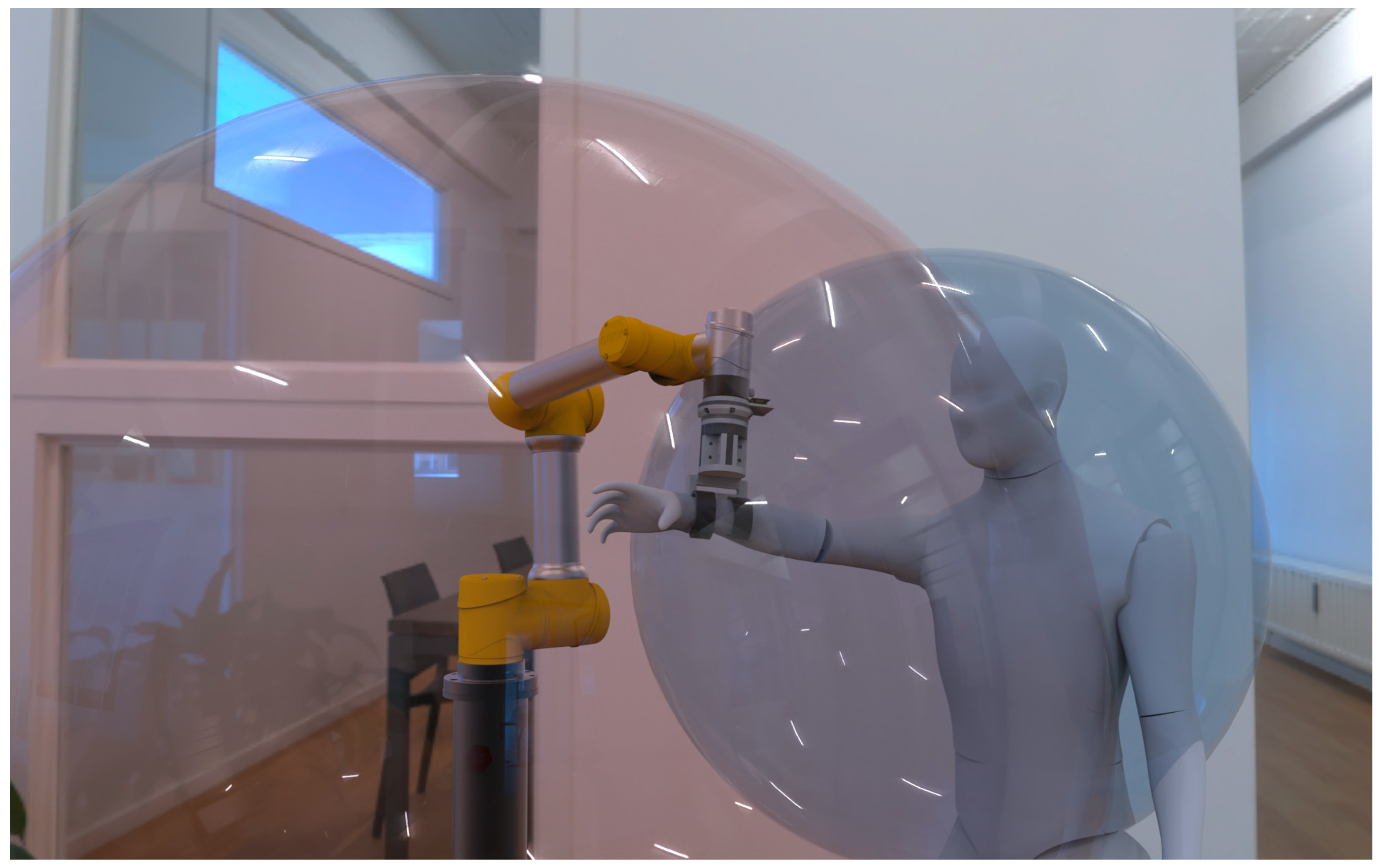
Figure 1. Conceptual schematic diagram of the virtual safe admittance boundary of a rehabilitation robot.
Applsci 13 05816 g001
Figure 2. Overall flowchart of the safe admittance boundary algorithm.
Applsci 13 05816 g002
Figure 3. Method for point cloud isodensification in the FK model.
Applsci 13 05816 g003
Figure 4. (a) Euclidean distance in the nearest neighbor search; (b) point cloud visualization based on nearest neighbor density.
Applsci 13 05816 g004
Figure 5. Space classification model constructed based on the nearest neighbor density of the point cloud.
Applsci 13 05816 g005
Figure 6. Control layer of the variable stiffness admittance strategy.
Applsci 13 05816 g006
Figure 7. Experimental workflow.
Applsci 13 05816 g007
Figure 8. Test logic behind the space verification experiments.
Applsci 13 05816 g008
Figure 9. Platform for the space verification: (a) non-powered linkage mechanism with 4 DOFs and low damping and six–dimensional force sensor (ROBOTIQ FT–300); (b) visualization of the robotic simulation system.
Applsci 13 05816 g009
Figure 10. Point cloud data obtained from DAS: (a) definition of DOF of the kinematic model for DAS; (b) point cloud of DAS’s workspace generated using the Monte Carlo method; (c) point cloud of DAS’s workspace obtained by voxel center filtering; (d) four-dimensional combined point cloud obtained by the space classification model.
Applsci 13 05816 g010
Figure 11. Visualization of the space classification model based on DAS: (a) visualization of the dangerous space; (b) visualization of the boundary space; (c) visualization of the HRI space.
Applsci 13 05816 g011
Figure 12. Six–dimensional force data from the wrist joint of experimenter 1: (a) six–dimensional force data 1; (b) six–dimensional force data 2; (c) six–dimensional force data 3; (d) six–dimensional force data 4.
Applsci 13 05816 g012
Figure 13. A segment of F x variation curve and the velocity response curve of the moving point in the end–effector under different stiffness. (a) the six-dimensional force FX after interception and filtering for data 1; (b) the velocity response curves output from the admittance model with different virtual stiffness parameters.
Applsci 13 05816 g013
Figure 14. Visualization of the trajectories of the moving point in the end–effector with the input of the same six–dimensional force data with and without the application of the safe admittance boundary in the robotic simulation system.
Applsci 13 05816 g014
Table 1. Space verification results.
Side Length of the
Voxel Grid (m)
Average Judgment Time
(ms)
Success Rate
(%)
r 1 = r 2 = 0.02 11.6099.00
r 1 = r 2 = 0.04 9.9898.80
r 1 = r 2 = 0.06 5.7298.40
Table 2. Out–of–bounds simulation results.
Tester
Number
Number of
Experiments
Maximum Response Time
(ms)
Average Response Time
(ms)
14165.63161.54
24162.59159.64
34170.84161.91
44167.12162.80
54161.91158.44
Average4165.62160.87
Disclaimer/Publisher’s Note: The statements, opinions and data contained in all publications are solely those of the individual author(s) and contributor(s) and not of MDPI and/or the editor(s). MDPI and/or the editor(s) disclaim responsibility for any injury to people or property resulting from any ideas, methods, instructions or products referred to in the content.