A Novel Spatiotemporal Analysis Framework for Air Pollution Episode Association in Puli, Taiwan

Abstract

Air pollution has been a global issue that solicits proposals for sustainable development of social economics. Though the sources emitting pollutants are thoroughly investigated, the transportation, dispersion, scattering, and diminishing of pollutants in the spatiotemporal domain are underexplored, and the relationship between these activities and atmospheric and anthropogenic conditions is hardly known. This paper proposes machine learning approaches for the spatiotemporal analysis of air pollution episode associations. We deployed an internet of low-cost sensors for acquiring the hourly time series data of PM_2.5 concentrations in Puli, Taiwan. The region is resolved into 10 × 10 grids, and each grid has an area size of 400 × 400 m². We consider the monitored PM_2.5 concentration at a grid as its gray intensity, such that a 10 × 10 PM_2.5 image is obtained every hour or a PM_2.5 video is obtained for a time span. We developed shot boundary detection methods for segmenting the time series into pollution episodes. Each episode corresponds to particular activities, such as pollution concentration, transportation, scattering, and diminishing, in different spatiotemporal ways. By accumulating the concentrations within the episode, we generate a condensed but effective representation for episode clustering. Three clustering approaches are proposed, ranging from histogram-, edge-, and deep-learning-based. The experimental results manifest that the episodes contained in the same cluster have homogeneous patterns but appear at different times in a year. This means that some particular patterns of pollution activities appear many times in this region that may have relations with local weather, terrain, and anthropogenic activities. Our clustering results are helpful in future research for causal analysis of regional pollution.

1. Introduction

The economic development of human society has improved our living convenience; however, it has inevitably contributed devastating pollutants to our natural environment, such as in the air, soils, and water. There is a global consensus to set goals and take actions to prevent the environmental situation from worsening. In light of this, the United Nations (UN) has set up 17 Sustainable Development Goals (SDGs) [1] in 2015 to urge all the nations on the globe to take actions for reaching prosperous human well-being and performance into the future. Environmental protection is the core notion because it coincides with many of the SDGs, including good health and well-being (Goal 3), clean water and sanitation (Goal 6), affordable and clean energy (Goal 7), decent work and economic growth (Goal 8), sustainable cities and communities (Goal 11), responsible consumption and production (Goal 12), and climate action (Goal 13). Air is the most primitive element for living, and we inhale the air into our lungs every minute for respiration. It is significant that the World Health Organization (WHO) reported that more than 3 million premature deaths are caused by air pollutants every year [2].

Due to the extremely small volume size, the ambient PM_2.5 aerosols (particulate matter with an aerodynamic diameter ≤ 2.5 μm) could be inhaled into the human respiratory system and cause diseases. PM_2.5 aerosols could be generated in three ways: by natural phenomena, anthropogenic activities, and precursor emissions [3]. Natural phenomena such as soiling, crustal elements, volcanic eruptions, and sea salt drifting, result in coarser particles [4]. Anthropogenic activities ranging from vehicle exhaust, biomass burning, coal, and gasoline combustion to petrochemical production and steel refineries generate finer-sized particles. The last source is contributed by the photochemical transformation of precursor emissions such as sulfur dioxide (SO₂) and nitrogen oxides (NO_x).

Most of the existing research on air pollution places its focus on source apportionment, PM_2.5 concentration prediction, and spatiotemporal analysis [5,6]. The source apportionment research intends to identify the chemical compositions of the captured pollutants so that the suspicious emitting site may be detected. The receptor model, source model, and tracer model are the most prevalent apportionment methodologies [5]. The research for PM_2.5 concentration prediction is categorized into short-term (in hours or days), middle-term (in months or seasons), and longer-term (in years). The most commonly applied methodologies are mathematical regression, machine learning, and meta-evolution [7]. As compared to source apportionment and concentration prediction, the research for spatiotemporal analysis is less contemplated. This is mainly because of the high computational effort incurred by combining spatial and temporal data for pattern discovery. Most researchers applied classic statistical approaches to describe the general properties of the data, and they conducted regression separately on spatial and temporal axes to save computational time [8,9]. Only a few studies [10,11] employed machine learning techniques to identify spatiotemporal clusters of similar PM_2.5 dispersion patterns, leaving a large room for deeper exploitation.

This paper proposes an innovative spatiotemporal analysis framework for air pollution episode association. Our methodology is unique in the sense that we develop the air pollution spatiotemporal analysis from the perspective of video analysis. The crossover between the two fields creates new and innovative techniques that bring many insights unseen before. If we take a bird’s-eye view of the land from above and monitor the hourly PM_2.5 concentrations, the geography becomes an image map if we consider the quantity of PM_2.5 concentrations as the gray value of pixels. The air pollution time series then becomes a video that can be analyzed using novel video processing techniques. We developed the shot boundary detection algorithms to separate the air pollution time series into meaningful shots (video clips). Each shot implicitly corresponds to an air pollution episode that may contain patterns of pollution accumulation, transportation, and dispersion. To represent the pollution episode efficiently and effectively, the gait energy image (GEI) scheme is adopted to digest the shot characteristics into a single image. We then applied the clustering algorithms to partition the GEIs produced from the air pollution time series into insightful groups that reveal that the main pollution episodes are related to the local terrain, climate, and anthropogenic activities. With the results, effective strategies for reducing air pollutants can be managed.

The remainder of this paper is organized as follows. Section 2 reviews the relevant research on air-pollution spatiotemporal analysis and the video analysis techniques that are relevant to our proposed methodology. Section 3 elucidates the proposed spatiotemporal analysis framework and the developed algorithms. Section 4 presents the experimental results and comparative performances. Finally, Section 5 concludes this work.

2. Literature Review

2.1. Air-Pollution Spatiotemporal Analysis

The classic approaches for air-pollution spatiotemporal analysis fall into four categories.

(1) Correlation and variance. The basic spatiotemporal relationship between PM_2.5 concentrations monitored at different sites along a time span can be realized by calculating the correlation coefficient (CC) and coefficient of variance (CV). Song et al. [12] profiled the spatiotemporal distribution of air pollution characteristics in Jiangsu Province, China, by investigating correlation and variance statistics such as the temporal and spatial air quality index (AQI) variations, the temporal correlation between AQI and meteorology, and the correlation between major pollutants. Lung et al. [6] calculated CV among different sites within a city. A higher CV indicates a greater fluctuation in PM_2.5 concentrations in a city. The distribution of CV among ten community locations was analyzed. It is seen that more than one-fifth of the time in July and December, the CV exceeds 20%. The majority of cases appear on weekends, mainly due to traffic, restaurants, and temples. It conforms to the activities attended by the inbound tourists. The CC between microsites and the nearest supersite was evaluated in [6] to validate the consistency of pollution patterns at highly correlated sites. Yang et al. [13] investigated the CC between PM_2.5 concentrations/variations and the urbanization level of the city. Their result manifests a positive/negative correlation between urbanization and PM_2.5 concentrations/variations.

(2) Spatiotemporal regression. Regression has been widely applied to find the relationship between the response variable and independent variables. Several studies have attempted to find the regression expression between PM_2.5 concentrations and multiple independent variables (such as meteorological or socioeconomic data). To reduce the model computations, Lung et al. [8] and Liu et al. [9] applied spatial regression to neighboring monitoring sites and economic variables at a particular time period. Yang et al. [13] applied quadratic spatial regression to disclose the contribution to PM_2.5 concentrations by urbanization, industrialization, and green land area.

(3) Probabilistic approaches. To model the spatiotemporal variations of PM_2.5 concentrations, both parametric and non-parametric probability distributions have been employed. Jiang et al. [14] used a two-parameter gamma distribution to describe the probability density functions (PDFs) of the hourly surface PM_2.5 concentrations in each city over seasonal time frames. The two parameters are referred to as the shape parameter and the scale parameter, whose optimal values are determined by fitting the historical data. Yu and Wang [15] assumed a yearly-invariant spatiotemporal distribution of the PM_2.5/PM₁₀ ratio at the same location during the same period of a year. Hence, the historical data of PM_2.5/PM₁₀ ratios can be used to construct a non-parametric distribution for predicting PM_2.5 if the PM₁₀ observation is available.

(4) Machine learning. Compared to the references using previously noted spatiotemporal analysis methods, the adoption of machine learning approaches has received more attention recently. Cao et al. [11] considered the hourly PM_2.5 concentrations in each day as a 24-dimension vector and applied the agglomerative hierarchical clustering approach to partition the PM_2.5 time series into four groups. They identified that the first group contains those days with severe pollution, the second group corresponds to the dispersion period, the third group coincides with the pollution accumulation period, and the air is relatively clean during the days included in the last group. Cao et al. [11] further applied the entropy weight method (EWM) to calculate the weighted mean PM_2.5 of the four clusters for each monitoring site in the city, where the cluster weight is given by the reciprocal entropy. The weighted mean PM_2.5 can be used to identify the PM_2.5 hotspots in the city. Yan et al. [10] used a spatially adjacent matrix and the PM_2.5 concentrations tallied by all the monitoring sites in 13 cities in the Beijing-Tianjin-Hebei (BTH) region to conduct a spatial clustering analysis. Their study showed that the PM_2.5 spatial homogeneity is highest in winter and lowest in summer, and for the same time period, the PM_2.5 spatial variations increase from southeast to northwest of the BTH region. Lyu et al. [16] systematically examined the spatiotemporal variations of air pollutants in the BTH region and then applied the random forest model and the decision tree regression for predicting spatiotemporal variations of pollution concentrations. It is found that the importance of factors influencing prediction performance depends on the spatial trend of variations.

In addition to the four categories of spatiotemporal analysis approaches, it is worth noting that hybrid methods exist in order to synergize the benefits gained by different approaches. For example, Chicas et al. [17] proposed a hybrid method that combines different spatiotemporal analysis approaches to make the interpretation of pollution dynamics more complete. The method analyzes the spatiotemporal distribution, trend, forecast, and factors about the air pollutants in Nagasaki Prefecture, Japan, by using correlation, auto-regressive, and machine learning techniques to offer a holistic perspective about the pollution dynamics.

There are several drawbacks to the existing PM_2.5 spatiotemporal methods. (1) Due to the high complexity of computation, traditional methods conduct spatial and temporal analysis separately. However, the higher-level correlation existing in the intertwined spatiotemporal domain is neglected in such separate analyses. (2) Existing methods design PM_2.5 spatiotemporal analysis on a piece-by-piece basis, lacking a comprehensive view to elucidate the linkage between different spatiotemporal analysis functions. (3) Most existing methods employ statistical approaches; only a small number of works have attempted machine learning techniques to group PM_2.5 time series into typical variation patterns, overlooking the benefits that may be contributed by abundant machine learning techniques. In this paper, we propose a novel design for comprehensive PM_2.5 spatiotemporal analytics that automatically cuts the PM_2.5 spatiotemporal time series maps into pollution episodes and then clusters those episodes into groups based on pollution spatiotemporal patterns. The analyzed result discloses that similar pollution episode patterns appear in different time periods of the year. They can be used further to explain the relationship between air pollution patterns and local meteorological and anthropogenic factors. Our design is based on video analysis techniques described as follows.

2.2. Video Analysis

Video is a time series of image frames, and it is by nature a spatiotemporal stream of data. The existing techniques for video processing have many analogies with the methods for air-pollution spatiotemporal analysis. In particular, the shot boundary detection (SBD) techniques, the gait energy image (GEI) representation scheme, the image retrieval algorithms, and the convolutional neural networks (CNN) are most relevant to our proposed methods, and they are reviewed as follows:

(1) Shot boundary detection (SBD). Video is a stream of image frames. To deliver situated semantics, a video is composed of a sequence of scenes, and each scene may have one or more shots. Each shot contains contiguous image frames that are uninterruptedly shot by a camera to represent continuous actions in time and space. Video SBD is the temporal segmentation of a video into consecutive shots that are primitive elements for video indexing and retrieval [18,19,20]. The video shot boundary appears in the frame(s) transiting from one shot to another shot. The transition between two consecutive shots usually appears in two types. The abrupt transition (hard cut) is a significant and sudden change from one shot to the next. The soft transition (soft cut) is a gradual change between the adjacent shots by applying spatial, chromatic, or spatial-chromatic effects, resulting in several stylish transitions such as dissolve, wipe, and fade in/out. Clearly, soft-cut detection is more challenging than hard-cut detection. Most existing SBD techniques proceed as follows: A score function is defined for estimating the probability of a frame being the true cut separating two consecutive shots. Then an appropriate threshold is used to classify the frames into cuts and non-cuts based on their scores.

Several score functions were developed [19,20]. (1) Sum of absolute differences (SAD). The score function sums up the absolute difference between corresponding pixels at the same location in the two consecutive image frames. This is the earliest SBD approach, which is simple but sensitive to object movement and may produce many false cuts. (2) Histogram differences (HD). Instead of computing the difference at the pixel level, the difference between the histograms of consecutive frames for each color channel is calculated. The HD is less sensitive to object movement. However, it loses the spatial information, i.e., the histogram of two completely different images can be exactly the same. (3) Edge change ratio (ECR). Since the cut appears at the frame(s) where the old edge pixels disappear and the new edge pixels emerge, the cut score can be estimated by calculating the difference at the edge locations. (4) Transform correlation (TC). The image frames are transformed into the frequency domain, and the correlation between the transformed images is evaluated. The cut frame is identified at the local minimum of the correlation. (5) Hybrid score functions (HSF) have been proposed by combing two or more of the above-mentioned approaches to enhance the robustness of the score function for different video contexts.

(2) Gait Energy Image (GEI). Human individual recognition in a natural scene is a very challenging problem because the image/video capturing the individual may just capture some parts of the individual (e.g., face, shoulder, waist, and legs) or from any viewing angle (front, side, bird’s-eye, and back). Therefore, various biometrics (face, fingerprint, and palm print) and context (posture, gait, and silhouette) were investigated to enhance the accuracy of human individual recognition. One of the novel context-based techniques for human individual recognition is the GEI technique proposed by Han and Bhanu [21]. GEI is a spatiotemporal representation to analyze human walking properties for individual recognition by gait. GEI represents human gait motion in a single image while preserving spatiotemporal information. The sequence of binary silhouettes of humans walking in the video was extracted from the original video. The GEI is the image obtained by calculating the mean gray image over all silhouettes in the time sequence. The GEI can be used to estimate the gait frequency and phase of a person for individual recognition.

(3) Image retrieval. The Bag-of-Words (BoW) model was originally proposed for the information retrieval of documents. The keywords contained in the documents are used to create a dictionary. Each document is represented by a vector describing the occurrence of each keyword in the document. As such, the document retrieval task can be transformed into similarity matching between vectors. Lee et al. [22] extended this idea to image retrieval by replacing the keywords with visual words that are the local visual features extracted from the images. The BoW model recognizes image categories by using a histogram of visual words to record the multiplicity of salient features. As there are many visual words, the vector quantization technique needs to be applied to construct a codeword dictionary in which the number of codewords is significantly lower than the number of visual words produced from all the images in the training set. Each visual word contained in an image is assigned the most relevant codeword according to the dictionary. The histogram, which counts the number of visual words assigned to each codeword, is used to represent the image for category recognition. The classifier is thus able to learn the category model of each generic object. It is found that the category model is robust against variations in viewing angles, illumination, scaling, and deformation.

(4) Convolutional neural networks (CNN). Artificial neural networks are computing systems that process signals via multiple layers of nodes, mimicking neurons in brain science. Rosenblatt [23] introduced feedforward neural networks (FNN), where the nodes receive signals from every node in the previous layer, process the signals, and forward the result to all the nodes in the next layer. The multilayer perceptron is the first successful model using FNN. As the number of hidden layers increases, it becomes computationally prohibitive to learn the network parameters. Hinton and Salakhutdinov [24] proposed deep belief networks (DBN), which simplify computations through multiple restricted Boltzmann machines. The CNN methods, which process signals based on convolution and downsize sampling, have emerged as the dominant neural network model for computer vision tasks. The CNN methods have won prizes in the ILSVR (ImageNet Large Scale Visual Recognition Competition). Some of the prize-awarded CNN methods are AlexNet [25], VGG-19 [26], and ResNet [27]. Considering the recognition accuracy and computation efficiency, we will employ VGG-19 for the episode clustering in this paper.

3. Proposed Methods

3.1. Framework Architecture

Figure 1 shows the framework architecture of the proposed methods. The innovations in our methods rely on the use of video processing techniques that have never been applied to air-pollution analytics. We discover there is a great analogy between the episodes of PM_2.5 activities and the shots of video scenes. The data acquisition and conversion method obtains the long-term air-quality concentration time series, which is then converted to a 10-category air-quality alert time series for episode analysis. The time series is actually a video when considering the air-quality alert category as pixel intensity level. The cycle of PM_2.5 episodes—pollution accumulation, transportation, dispersion, and diminishing—can be considered as various shots in the video. We developed four video shot detection algorithms for comparing the quality of the segmented episode shots. In a particular region, some salient meteorological phenomena and anthropogenic activities repeatedly happen. These patterns, if correctly extracted and grouped according to their similarity, would reflect the reasons that cause the major air pollution episodes that frequently appear in the monitored region. We first transform the shots into corresponding GEIs for efficient processing. Three GEI clustering algorithms are proposed to partition the GEIs into episode clusters. These clusters disclose interesting pollution patterns that are implicitly related to local climate and economic activities.

3.2. Air-Quality Data Acquisition and Conversion

The field study conducted in this paper is located in Puli, central Taiwan. Puli is a small town with an area of 13 × 13 km² and it is centered at 23°58′12″ north latitude and 120°58′12″ east longitude. The geography of Puli is basin terrain. There are three rivers flowing to the west coast of Taiwan and creating three valleys, which induce the transportation of air pollutants yielded in the west metropolis into the Puli basin. It is desired to analyze the main patterns of pollution emergence, including those resulting from external sources or local emissions. As such, appropriate pollution-free actions can be enforced by the public. Our studied field is the interior of the basin geography, which is resolved in 10 × 10 grids with an area of 8 × 8 km². Within each grid, we acquire the PM_2.5 concentration every hour. In our previous research [28], we had deployed 32 PM_2.5 sensors in some of the grids. The sensors are model G7 PMS7003, which uses a laser beam to illuminate the suspended air particles and generate light scattering. The scattered light is then analyzed to estimate the particle size and the number of particles. For those grids where there are no sensors, the concentration intensity can be simulated by smoothing the concentration intensity from nearby sensors or applying machine-learning imputation techniques such as the one suggested in Yin et al. [21]. Hence, for every hour, we obtain an image frame of n × n pixels, and the PM_2.5 concentrations in the grids are considered the gray values of the image. If we continuously monitor the PM_2.5 concentrations in Puli for 365 straight days, we will produce a time series of 365 × 24 = 8760 image frames, which is a video. In this paper, we acquired the hourly PM_2.5 concentrations from the PM_2.5 sensors from 1 January 2018 until 31 December 2018, so the collected data involve four seasons. To extract salient and meaningful PM_2.5 episodes, the concentrations of image pixels are converted to those with 10 air-quality alert levels, as shown in Figure 2. As the original six air-quality alert categories defined by the Taiwan Environmental Protection Administration (EPA) may not be sufficient to describe the dynamic variations of air pollution activities, we refine the six-level categories to 10-level categories. Next, we propose pollution episode segmentation methods with the alert category time series video.

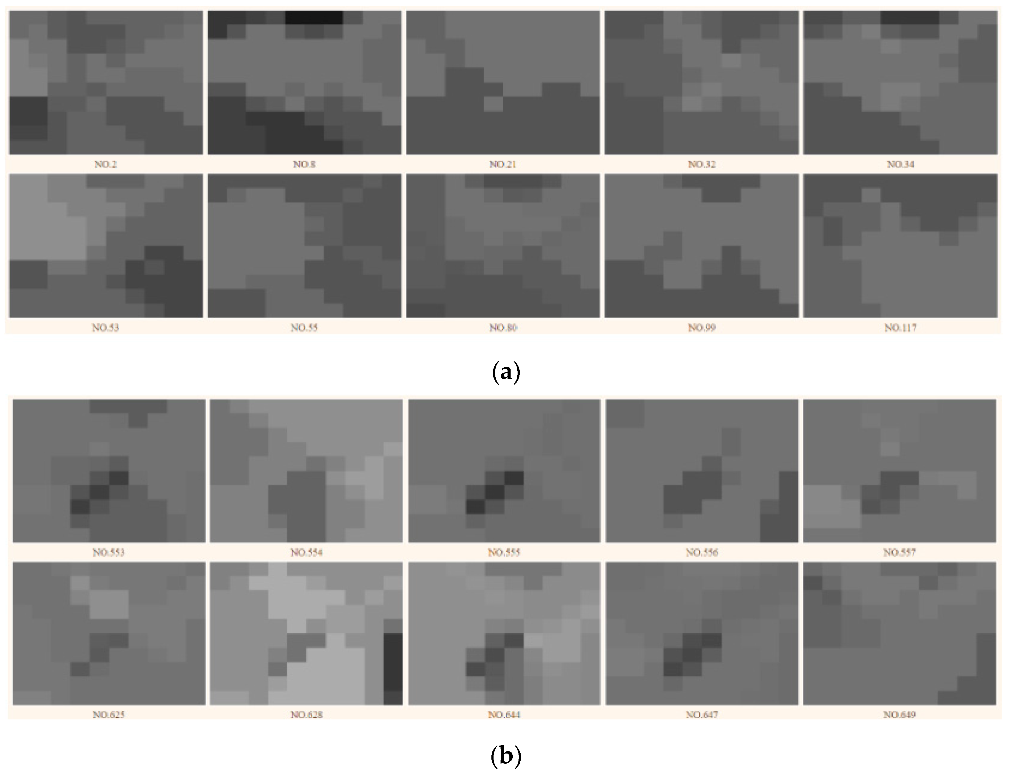
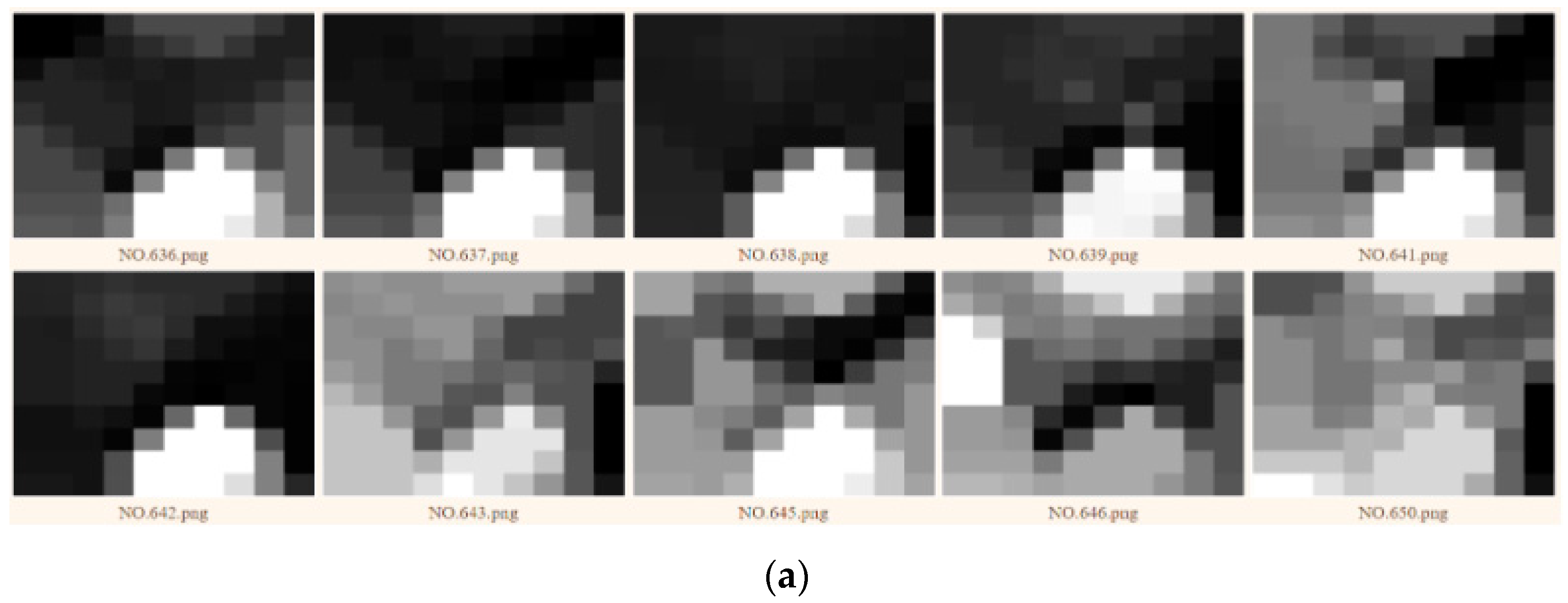
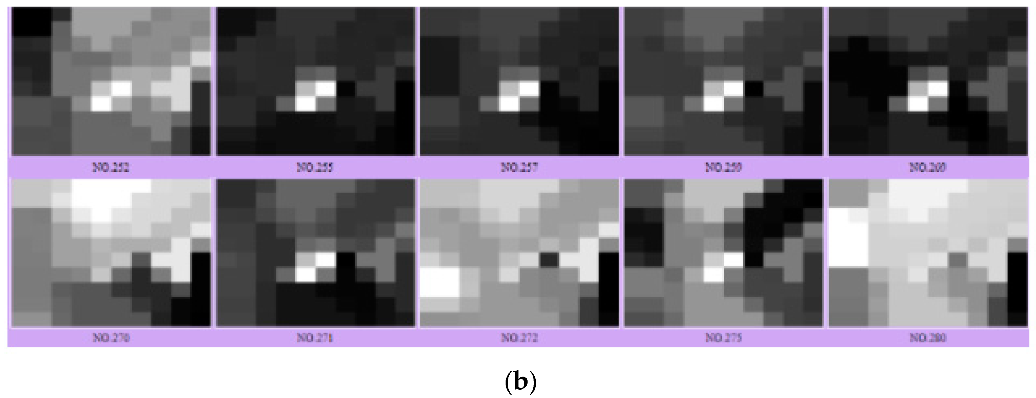
3.3. Pollution Episode Segmentation

We developed the shot boundary detection (SBD) algorithms to separate the alert category time series maps into meaningful shots (video clips). Each shot implicitly corresponds to an air pollution episode, which may contain patterns such as pollution accumulation, transportation, dispersion, and diminishing. We expect that the alert category maps contained in the same shot are more homogeneous than those falling in different shots. The activity of air pollution is very complex and related to multi-criteria such as land terrain, weather, and anthropogenic activities. There is no clear definition of how many types of air pollution patterns are observed in a place. Some ideal examples are ‘clean and stable’, ‘pollution emerging’, ‘pollution transportation’, ‘pollution dispersion’, and ‘pollution dissipating’. However, there still exist other patterns that need to be explained by investigating natural and anthropogenic criteria.

We propose four types of shot boundary detectors, as follows:

(1)

Raster Difference (RS). The RS method reserves all of the n × n grid values in a raster-scan order and calculates the difference of the corresponding grid values between different frames within a time window. The sum of the raster differences over the entire frame is compared to a threshold for shot detection.

(2)

Histogram Difference (HD). Instead of reserving the raster sequence of grid values, the HD method constructs a histogram by counting the number of grids having each level of the 10 alert categories. The 10 occurrence numbers on the histogram are used as the feature vector to calculate the difference between different frames within a time window. As compared to the RS method, the HD method is less sensitive to rotation and translation of the same pollution patterns and is more likely to extract complete shots of various episodes.

(3)

Edge Difference (ED). The ED method applies the Sobel edge detectors, which are commonly used in the field of image processing, to extract the boundaries between adjacent grids having significantly distinct PM_2.5 alert categories. The implementation of the ED method is motivated by the assumption that the edge orientation of the pollution region changes abruptly at the transition to the next episode. The four 3 × 3 Sobel edge filters, as depicted in Figure 3, for extracting vertical, horizontal, and two diagonal edges are employed to convolute the frame image. The response at each pixel to the four filters is summed up to obtain 64 edge response values as the feature vector, which is used to calculate the difference between different frames.

(4)

Statistics Based (SB). The SB method extracts the properties of the alert category map and detects the cutting frames, which are assumed to have large variations in these properties as compared to the frames in the next shot. In particular, we use six moment statistics; three are non-positional and the others are positional. Let the position of the n × n grids be resolved as a two-dimensional array, and the grid value at position [x, y] is denoted as g[x, y]. The three non-positional moments are as follows:

$$\frac{1}{n^2}{{\displaystyle \sum }}_{x=1}^n{{\displaystyle \sum }}_{y=1}^n{\left(g\left[x,y\right]-\overline{g}\left[x,y\right]\right)}^k, k=1, 2, 3$$

(1)

where $\overline{g}\left[x,y\right]$ is the mean of g[x, y] over all n × n grids.

On the other hand, the positional moments designed in this paper are calculated by multiplying the grid moment element with the weighting of positional indices.

$$\frac{1}{n^2}{{\displaystyle \sum }}_{x=1}^n{{\displaystyle \sum }}_{y=1}^n\left({\left(g\left[x,y\right]-\overline{g}\left[x,y\right]\right)}^k\times \left(ax+b^y\right)\right), k=1, 2, 3$$

(2)

where a and b are the parameters for tuning the linear and exponential weightings at position [x, y].

Our PM_2.5 episode segmentation algorithms detect episode boundaries (cuts) to separate the alert category time series into meaningful shots. To evaluate the correctness of the segmented shots, each image frame in the time series was labeled as cut or non-cut by an expert who has worked in this area for three years. In the machine learning literature, the commonly used performance measures, namely, precision, recall, and F1-Score, for a two-class classification problem (cut or non-cut in our case) are as follows:

$$Precision=\frac{TP}{TP+FP}$$

(3)

$$Recall=\frac{TP}{TP+FN}$$

(4)

$$\mathrm{F}1-\mathrm{Score}=\frac{2\times Precision\times Recall}{Precision+Recall}$$

(5)

where TP, FP, and FN are the numbers of true positive, false positive, and false negative samples, respectively.

Each of the measures gauges the classification’s performance from a different perspective. Precision focuses on the classification correctness of the samples that the algorithm recognizes as positive, while recall emphasizes how many true positive samples are correctly recognized by the algorithm. Precision and recall are contrasting measures. A perfect recall can be obtained at the cost of reduced precision by letting the algorithm recognize more samples as positive with a lower classification threshold value. The F1-Score is a balance measure that takes into account both precision and recall simultaneously.

After performing the SBD methods on the PM_2.5 alert category time series, a number of episode shots are obtained. Each shot is a sequence of alert category maps within a time period and potentially elucidates a particular pollution episode. To efficiently represent the pollution episode shot, the gait energy image (GEI) scheme is adopted to reserve the main pollution variations in the spatiotemporal domain in a single image. GEI representation was proposed in [19], where the human walking gaits are extracted for individual recognition. The GEI is the image obtained by calculating the mean gray image over the sequence of human walking videos in the time sequence. In the context of our research, the GEI is the mean gray image over the sequence of alert category maps in the segmented shot.

3.4. Pollution Episode Clustering

We then applied the clustering algorithms to partition the GEIs produced from the air pollution time series into insightful groups, which reveal the main pollution episodes related to the local terrains, climate, and anthropogenic activities. With the results, effective strategies for reducing air pollutants emitted from anthropogenic activities can be managed. Both atmospheric and anthropogenic conditions have cyclic patterns. For instance, those atmospheric phenomena ranging from seasonal monsoons and tropical cyclones to temperature inversions during a day are commonly seen atmospheric cyclic patterns that affect the concentrations and dispersions of air pollutants. Analogously, many anthropogenic activities also manifest cyclic conditions, such as rush/off-peak hours, weekdays/weekends/holidays, crop burning, and electricity consumption, which would entail cyclic pollution patterns. The transportation and scattering of the pollutants monitored at local microsensors manifest particular patterns related to local terrains such as rivers, plateaus, mountains, and residential areas. As the GEIs constitute the spatiotemporal drifting of air pollutants, we anticipate that some GEIs are more homogeneous under similar atmospheric and anthropogenic scenarios than those in different ones. In order to probe into the cyclic patterns of local air pollutants, the extracted GEIs are grouped into clusters. We propose three GEI clustering approaches, namely, the histogram vectors (HV), bag of words (BoW), and convolutional neural networks (CNN), as follows.

(1)

HV. Following the same fashion as our HD method, a histogram is constructed by counting the number of grids having each level of the 10 alert categories. The 10 occurrence numbers on the histogram are used as the feature vector for conducting the k-means clustering method. To evaluate the quality of the clustering result, several different numbers of clusters are specified when conducting k-means clustering.

(2)

BoW. BoW was originally proposed for document retrieval by using keywords, and it has been extended for image retrieval by replacing the keywords with visual words [20]. We further extend this idea for GEI image clustering. We associate Sobel edge filters with visual words. The GEI is divided into four quadrants. Every quadrant is processed by the four 3 × 3 Sobel filters for extracting horizontal, vertical, and diagonal edges. The response values for the same filter within every quadrant are summed up to simulate the occurrence count of the corresponding visual word. As such, we obtain a 4(quadrant) × 4(filter) = 16 visual-word histogram. Furthermore, the histogram is used as the feature vector for the k-means clustering method.

(3)

CNN. In contrast to HV and BoW, which learn prespecified features designed by human experts, CNN automatically learns the representative features for the designated task. In particular, we apply VGG-19 [26] by using Keras. VGG-19 was trained with one million images selected from the ImageNet dataset for classification into 1000 generic classes. VGG-19 has 16 convolutional layers with a large number of filters, followed by three fully connected layers. We fed VGG-19 with all GEIs and summed up the collected softmax values for each classification class. The top 20 softmax-value classes are used to construct features for GEI clustering. Further, each GEI obtains a 20-dimensional feature vector, and the k-means clustering method is applied to the feature vectors to generate the clustering result.

In order to evaluate the performance of the proposed three GEI clustering methods, namely, the HV, BoW, and CNN, we need to find appropriate measures. Unfortunately, as clustering is an unsupervised learning task, there is no universal measure for justification of the clustering result. The most widely used measures are the silhouette coefficient (SC), the Calinski-Harabaz index (CHI), and the Davies-Bouldin index (DBI), as defined as follows:

Let the N data points be grouped by the applied clustering algorithm into k clusters, each with n_i points, i = 1, 2, …, k. The SC [29] is the mean of the silhouette width for each point. The silhouette width S(j) for point j is defined as

$$S\left(j\right)=\frac{b\left(j\right)-a\left(j\right)}{max\left(b\left(j\right), a\left(j\right)\right)}$$

(6)

where a(j) is the mean distance from point j to every other point assigned to the same cluster, and b(j) is the distance from point j to its nearest neighbor assigned to any different cluster. The SC is then given by

$$SC=\frac{{{\displaystyle \sum }}_{j=1}^{N}S\left(j\right)}{N}$$

(7)

The value of the silhouette coefficient, SC, ranges from −1 to 1. The higher the SC, the more appropriate the clustering result.

The CHI [30] measures cluster validity in terms of between-cluster and within-cluster distances. Let’s denote the centroid of cluster i by m_i. and the centroid of all clusters by m. The between-cluster square distance (SSB) and the within-cluster square distance (SSW) are defined as follows:

$$SSB={{\displaystyle \sum }}_{i=1}^k{n}_i\parallel m_i-m\parallel {}^2$$

(8)

$$SSW={{\displaystyle \sum }}_{i=1}^k{{\displaystyle \sum }}_{j=1}^{n_i}\parallel x_{ij}-m_i\parallel {}^2$$

(9)

where $x_{ij}$ is the coordinate vector of point j in cluster i. The CHI is then given by

$$CHI=\frac{SSB}{SSW}\times \frac{N-k}{k-1}$$

(10)

The higher the CHI is, the more valid the partition with clustering.

In contrast to CHI, which measures the mean SSB and SSW, the DBI [31] measures the ratio between the individual SSW of a cluster and its SSB to every other cluster. The DBI is calculated as follows:

$$DBI=\frac{1}{k}{\displaystyle \sum }_{i=1}^{k}ma{x}_{i\ne j}\frac{\sqrt{{{\displaystyle \sum }}_{h=1}^{n_i}\parallel x_{ih}-m_i\parallel {}^2}+\sqrt{{{\displaystyle \sum }}_{h=1}^{n_i}\parallel x_{jh}-m_j\parallel {}^2}}{\sqrt{\parallel m_i-m_j\parallel {}^2}}$$

(11)

The smaller the DBI, the more preferable the clustering result.

4. Experimental Results and Comparative Performances

4.1. Pollution Episode Segmentation

The comparative performances of the proposed episode segmentation algorithms in terms of the three measures are tabulated in

Table 1. Comparative performances of the proposed episode segmentation algorithms.

	Precision	Recall	F1-Score
RS	0.7225909	0.74270123	0.732508063
HD	0.6956363	0.78076398	0.735745954
ED	0.55856833	0.702592087	0.622356495
SB	0.6792861	0.68540246	0.682330574

. It is seen that RS and SB have more balanced performance on precision and recall than HD and ED. This is a desired property because false positives from cuts will result in many short shots without delivering meaningful episodes, which hinder the explanation of complete pollution cycles. On the other hand, RS and HD are overall better performers whose F1-Score is above 73%, followed by SB, which obtains an F1-Score of 68%. The worst performer among the four competing methods is ED, whose F1-Score is 62%. The reason for the performance ranking may be due to the low resolution and shallow color depth of the air-pollution alert map, which is resolved as a 10 × 10 image with only 10 pollution-alert color categories. The edge information and moment statistics of such an image are not sufficient for effectively differentiating the difference between cut and non-cut frames. Another disadvantage of ED is that the edge responses are relative values rather than absolute ones, and it cannot tell the difference in the edge between category 1 and category 2 or between category 9 and category 10, explaining why ED is the worst performer.

In Figure 4, we show the detected cuts and the true labeled cuts on an example time sequence by using the proposed episode segmentation methods. The true labeled cuts are marked with a red border, while the cut determined by the applied method is marked with a black border. When the true labeled cut is correctly detected by the applied method, the cut is marked with both red and black borders. It is observed that there are nine true labeled cuts out of 80 frames in the time sequence. The nine true labeled cuts belong to three soft transitions, which segment the time series into four meaningful pollution episodes. The RS, HD, ED, and SB detect 5, 6, 14, and 13 cuts, respectively. This reveals that ED and SB may tend to produce more short episodes. A promising phenomenon is that the three soft transitions are detected by all methods, with at least one cut-frame detected within each soft transition. ED and SB may produce more cuts than the true labeled cuts. However, if we examine these cuts closely, the true cuts labeled by the experts are intended to segment the complete pollution cycle consisting of concentration accumulation, transportation, and diminishing. While the cuts detected by ED and SB may produce shorter episodes such as concentration accumulation or pollution diminishing.

4.2. Pollution Episode Clustering

The segmented episodes implicitly correspond to spatiotemporal activities in a pollution cycle such as concentration accumulation, transportation, dispersion, and diminishing. Due to the local properties related to microclimate, land terrain, and anthropogenic activities, the pollution episodes have repeated patterns, such as emerging pollution concentrations from the downtown area, transporting pollution from the west river valley to the east, and scattering to larger areas before they diminish. It is desirable to group the episodes belonging to the same pollution pattern in a cluster for further causal analysis. However, a pollution episode is a sequence of images. It is difficult to cluster episodes directly. GEI is an effective representation scheme that compresses a short video into an image while still preserving the main scene-changing dynamics in the video. We thus transform the segmented episodes into GEIs.

Figure 5 shows an illustration for constructing the GEI from a given PM_2.5 episode. The episode consists of a time series of eight pollution hourly maps, as shown in the first two rows, and the image in the last row is the constructed GEI. It is seen from the episode series that the orange-alert pollution emerges from the upper-right towards the lower-left until it almost covers the entire map (see the fifth hour image). At the sixth hour image, a red-alert pollution appears in the upper-center and lasts for two hours. Finally, at the eighth hour image, the pollution is reduced to orange-alert. This episode shows many dynamics of the pollution cycle, including concentration accumulation (between the first and third hours), dispersion (between the fourth and fifth hours), intensification (at the sixth hour), and reduction (between the seventh and eighth hours). By accumulating the intensity over the eight image maps, the episode is condensed to a GEI image, as shown in the last row. The darkest cells indicate the constantly lower PM_2.5 intensity observed during the whole duration of the episode, while on the contrary, the brighter area manifests the continuingly high PM_2.5 concentrations in the episode. The various intermediate gray levels correspond to the changing dynamics of PM_2.5 concentrations during the time span of the episode. The brightest cells in the upper center indicate there was serious pollution in this region. GEI is a condensed representation of an episode, and it reserves information about the main pollution dynamics observed in the episode.

Now we proceed to the clustering of the GEIs into groups such that the GEIs assigned to the same group manifest similar pollution dynamics, and the comparative analysis conducted on these GEIs may disclose the multi-factors (terrains, climate, anthropogenic activities, etc.) that result in the particular pollution dynamics. We evaluate the performance on GEI clustering obtained by the proposed HV, BoW, and CNN methods. The specified number of clusters, k, ranges from 2 to 9. The SC, CHI, and DBI derived for each competing method are listed in

Table 2. The clustering performance of the HV method.

K	SC	CHI	DBI
2	0.501591138	600.3940942	1.108177263
3	0.647946873	1004.078699	1.352115359
4	0.692444416	1254.325130	1.805470173
5	0.699810907	1283.911012	1.857432596
6	0.621794592	1407.539037	1.537950880
7	0.617850347	1414.988043	1.664281480
8	0.567976152	1390.361033	1.288370949
9	0.563132577	1366.345924	1.295097528

,

Table 3. The clustering performance of the BoW method.

K	SC	CHI	DBI
2	0.301451198	265.2936270	0.837995961
3	0.374914193	276.7063533	0.893594959
4	0.352490637	267.9174494	0.966339562
5	0.361700044	295.2575573	1.107479698
6	0.282343080	305.9140231	1.074090025
7	0.277204879	305.1391090	1.059764619
8	0.283878016	292.5594372	1.020158004
9	0.257572259	285.0925611	0.984416778

and

Table 4. The clustering performance of the CNN method.

K	SC	CHI	DBI
2	0.426706271	681.1978051	1.142826628
3	0.312079422	566.5341183	0.861172038
4	0.268289956	493.324105	0.817149345
5	0.278307506	469.2196243	0.898008358
6	0.271767518	428.1691441	0.758196849
7	0.264814784	400.385274	0.77981305
8	0.245515484	379.3548626	0.778609268
9	0.230716353	359.9879666	0.774757245

. The best value in terms of each performance measure for determining the optimal number of clusters is printed in boldface. It is seen that the suggested number of clusters is 5, 7, or 2 for the HV method, 3, 6, or 2 for the BoW method, and 2, 2, or 6 for the CNN method. The best SC and CHI performance is achieved by HV, followed by CNN, while the best DBI performance is obtained by CNN. It is worth noting that none of the methods dominates any other in all measures for a particular k value. In other words, we cannot conclude which clustering method is prevailing.

Figure 6 shows some members of the first two GEI clusters generated by using the HV method. It is seen that the GEIs in the same cluster are more homogeneous than those in different clusters, indicating the effectiveness of the HV method. The first cluster is composed of the GEIs, which have a horizontal pollution strip in the middle. The second cluster contains the GEIs, which have relatively clean air (darker gray) at the center surrounded by pollution concentrations. Both clusters deliver specific, meaningful pollution episodes that are very helpful in causal analysis to disclose why this particular pattern of episodes repeatedly appears at different times of the year.

Figure 7 shows some members of the first two GEI clusters generated by using the BoW method. It should be noted that this is unsupervised clustering; the cluster order has nothing indicating its content. As a result, the first cluster produced by HV should not be associated with the first cluster generated by BoW or CNN. It is seen that the GEIs in the first cluster have serious pollution concentrations with very high intensity at the bottom center area. This is very likely incurred by particular weather scenarios or anthropogenic activities that repeatedly appear at different times of the year, so we see several episode GEIs grouped in this cluster. For the second cluster, the included GEIs also have a particular pattern at the center of the map. This particular pattern may indicate a complex dispersion route where the pollution goes across the horizontal middle but circumvents some center cells (with very dark intensity). The reason for this phenomenon should be further investigated by examining the local terrain and artificial constructions.

Figure 8 shows some members of the first two GEI clusters obtained by the CNN method. In the first cluster, the GEIs show very rich episode dynamics. There are triangular shapes near the map sides, but the intensity range of the triangles differs among different GEI members. Additionally, these GEI members may have similar transportation behaviors but carry distinct pollution-alert categories. This is inherited from the nature of VGG-19, which recognizes generic object classes without paying too much attention to the object’s color. For the GEIs contained in the second cluster, a square of four brighter cells appears at the center, with darker cells surrounding the square. This isolated white square at the map center indicates a hot spot of PM_2.5 pollution, while the gradually decreasing intensity of its surroundings may show the dispersion routes of the center pollution source. However, this pattern is quite different from the square pattern we observed in the second cluster generated by BoW, where the center square pattern is dark with bright surroundings. Again, the reason behind this complex phenomenon can only be disclosed by further investigating the atmospheric and anthropogenic conditions that cause it. For instance, temperature inversions, rush/off-peak hours, weekdays/weekends, and crop burning may all entail such a pattern.

As we have mentioned, we cannot conclude which method is the best overall based on the performance measures (see Table 2, Table 3 and Table 4). Hence, the clustering results from each method are worth further investigation. A better way to apply the result is to reserve the classes obtained from all methods and conduct a causal analysis with local criteria such as land terrain, weather, and anthropogenic activities. As such, some insightful and explainable pollution classes can be identified. Our future work will collaborate with atmospheric and environmental experts to discover the relationships between the obtained pollution classes and the natural and anthropogenic criteria.

5. Conclusions

In this paper, we have proposed a spatiotemporal analysis framework for air pollution episode association. Classic spatiotemporal analysis approaches are statistics-based. The contribution of our paper relies on machine learning approaches, which already have successful applications in the image and video processing domains. In our previous research, we built an internet of low-cost sensors for monitoring the hourly PM_2.5 concentrations in Puli, Taiwan. With this big volume of PM_2.5 data, we transform it into a video that consists of a time series of pollution image frames. To disclose the main pollution patterns in this area, several shot boundary detection algorithms are proposed to detect the cut-frames separating the pollution episodes in the time series. Each episode corresponds to particular activities, such as pollution accumulation, transportation, scattering, and diminishing, in different spatiotemporal ways. The GEI representation scheme is applied to render the spatiotemporal dynamics of the episode such that they are able to be dealt with by the clustering method. Three clustering approaches are proposed for episode clustering, ranging from histogram-based, edge-based, and deep-learning-based. The experimental results manifest that the episodes contained in the same cluster have homogeneous patterns that appear at different times in a year. This means that some particular patterns of pollution activities emerge many times in this region that may have relations with local weather, terrain, and anthropogenic activities. The research results provide a useful clue for the causal analysis of regional pollution in our future study.

References

1. United Nations Department of Economic and Social Affairs. The 2030 Agenda for Sustainable Development. Available online: https://sdgs.un.org/goals (accessed on 5 April 2023).
2. WHO Media Centre. Ambient (Outdoor) Air Pollution. 2022. Available online: https://www.who.int/en/news-room/fact-sheets/detail/ambient-(outdoor)-air-quality-and-health (accessed on 25 April 2023).
3. Singh, N.; Murari, V.; Kumar, M.; Barman, S.C.; Banerjee, T. Fine particulates over South Asia: Review and meta-analysis of PM2.5 source apportionment through receptor model. Environ. Pollut. 2017, 223, 121–136. [Google Scholar] [CrossRef]
4. Valerino, M.; Ratnaparkhi, A.; Ghoroi, C.; Bergin, M. Seasonal photovoltaic soiling: Analysis of size and composition of deposited particulate matter. Sol. Energy 2021, 227, 44–55. [Google Scholar] [CrossRef]
5. Liang, C.S.; Duan, F.K.; He, K.B.; Ma, Y.L. Review on recent progress in observations, source identifications and countermeasures of PM2.5. Environ. Int. 2016, 86, 150–170. [Google Scholar] [CrossRef]
6. Fontes, T.; Li, P.; Barros, N.; Zhao, P. Trends of PM2.5 concentrations in China: A long term approach. J. Environ. Manag. 2017, 196, 719–732. [Google Scholar] [CrossRef]
7. Yin, P.Y.; Yen, A.Y.; Chao, S.E.; Day, R.F.; Bhanu, B. A Machine Learning-based Ensemble Framework for Forecasting PM2.5 Concentrations in Puli, Taiwan. Appl. Sci. 2022, 12, 2484. [Google Scholar] [CrossRef]
8. Lung, S.C.C.; Wang, W.C.V.; Wen, T.Y.J.; Liu, C.H.; Hu, S.C. A versatile low-cost sensing device for assessing PM2.5 spatiotemporal variation and quantifying source contribution. Sci. Total Environ. 2020, 716, 137145. [Google Scholar] [CrossRef]
9. Liu, X.J.; Xia, S.Y.; Yang, Y.; Wu, J.F.; Zhou, Y.N.; Ren, Y.W. Spatiotemporal dynamics and impacts of socioeconomic and natural conditions on PM2.5 in the Yangtze River Economic Belt. Environ. Pollut. 2020, 263, 114569. [Google Scholar] [CrossRef]
10. Yan, D.; Lei, Y.; Shi, Y.; Zhu, Q.; Li, L.; Zhang, Z. Evolution of the spatiotemporal pattern of PM2.5 concentrations in China–A case study from the Beijing-Tianjin-Hebei region. Atmos. Environ. 2018, 183, 225–233. [Google Scholar] [CrossRef]
11. Cao, R.; Li, B.; Wang, Z.; Peng, Z.; Tao, S.; Lou, S. Using a distributed air sensor network to investigate the spatiotemporal patterns of PM2.5 concentrations. Environ. Pollut. 2020, 264, 114549. [Google Scholar] [CrossRef]
12. Song, R.; Yang, L.; Liu, M.; Li, C.; Yang, Y. Spatiotemporal Distribution of Air Pollution Characteristics in Jiangsu Province, China. Adv. Meteorol. 2019, 2019, 5907673. [Google Scholar] [CrossRef]
13. Yang, D.; Chen, Y.; Miao, C.; Liu, D. Spatiotemporal variation of PM2.5 concentrations and its relationship to urbanization in the Yangtze river delta region. China Atmos. Pollut. Res. 2020, 11, 491–498. [Google Scholar] [CrossRef]
14. Jiang, Z.; Jolley, M.D.; Fu, T.M.; Palmer, P.I.; Ma, Y.; Tian, H.; Li, J.; Yang, X. Spatiotemporal and probability variations of surface PM2.5 over China between 2013 and 2019 and the associated changes in health risks: An integrative observation and model analysis. Sci. Total Environ. 2020, 723, 137896. [Google Scholar] [CrossRef] [PubMed]
15. Yu, H.L.; Wang, C.H. Retrospective prediction of intra-urban spatiotemporal distribution of PM2.5 in Taipei. Atmos. Environ. 2010, 44, 3053–3065. [Google Scholar]
16. Lyu, Y.; Ju, Q.; Lv, F.; Feng, J.; Pang, X.; Li, X. Spatiotemporal variations of air pollutants and ozone prediction using machine learning algorithms in the Beijing-Tianjin-Hebei region from 2014 to 2021. Environ. Pollut. 2022, 306, 119420. [Google Scholar] [CrossRef] [PubMed]
17. Chicas, S.D.; Valladarez, J.G.; Omine, K. Spatiotemporal distribution, trend, forecast, and influencing factors of transboundary and local air pollutants in Nagasaki Prefecture, Japan. Sci. Rep. 2023, 13, 851. [Google Scholar] [CrossRef]
18. Koprinska, I.; Carrato, S. Temporal video segmentation: A survey. Signal Process. Image Commun. 2001, 16, 477–500. [Google Scholar] [CrossRef]
19. Cotsaces, C.; Nikolaidis, N.; Pitas, I. Video Shot Boundary Detection and Condensed Representation: A Review. IEEE Signal Process. Mag. 2006, 23, 28–37. [Google Scholar] [CrossRef]
20. Abdulhussain, S.H.; Ramli, A.R.; Saripan, M.I.; Mahmmod, B.M.; Al-Haddad, S.A.R.; Jassim, W.A. Methods and Challenges in Shot Boundary Detection: A Review. Entropy 2018, 20, 214. [Google Scholar] [CrossRef]
21. Han, J.; Bhanu, B. Individual recognition using gait energy image. IEEE Trans. Pattern Anal. Mach. Intell. 2006, 28, 316–322. [Google Scholar] [CrossRef]
22. Lee, F.F.; Fergus, R.; Torralba, A. Recognizing and learning object categories: Year 2007. In Proceedings of the 2007 IEEE Conference on Computer Vision and Pattern Recognition, Minneapolis, MN, USA, 17–22 June 2007. [Google Scholar]
23. Rosenblatt, F. The perceptron: A probabilistic model for information storage and organization in the brain. Psychol. Rev. 1958, 65, 386. [Google Scholar] [CrossRef]
24. Hinton, G.E.; Salakhutdinov, R.R. Reducing the dimensionality of data with neural networks. Science 2006, 313, 504–507. [Google Scholar] [CrossRef] [PubMed]
25. Krizhevsky, A.; Sutskever, I.; Hinton, G.E. ImageNet classification with deep convolutional neural networks. Commun. ACM 2017, 60, 84–90. [Google Scholar] [CrossRef]
26. Simonyan, K.; Zisserman, A. Very deep convolutional networks for large-scale image recognition. arXiv 2015, arXiv:1409.1556. [Google Scholar]
27. He, K.; Zhang, X.; Ren, S.; Sun, J. Deep Residual Learning for Image Recognition. In Proceedings of the IEEE Conference on Computer Vision and Pattern Recognition 2016, Las Vegas, NV, USA, 27–30 June 2016. [Google Scholar]
28. Yin, P.Y.; Tsai, C.C.; Day, R.F.; Tung, C.Y.; Bhanu, B. Ensemble learning of model hyperparameters and spatiotemporal data for calibration of low-cost PM2.5 sensors. Math. Biosci. Eng. 2019, 16, 6858–6873. [Google Scholar] [CrossRef] [PubMed]
29. Rousseeuw, P.J. Silhouettes: A graphical aid to the interpretation and validation of cluster analysis. J. Comput. Appl. Math. 1987, 20, 53–65. [Google Scholar] [CrossRef]
30. Calinski, T.; Harabasz, J. A dendrite method for cluster analysis. Commun. Stat. 1974, 3, 1–27. [Google Scholar]
31. Davies, D.L.; Bouldin, D.W. A Cluster Separation Measure. IEEE Trans. Pattern Anal. Mach. Intell. 1979, 1, 224–227. [Google Scholar] [CrossRef]
Figure 1. Framework architecture of the proposed methods.
Applsci 13 05808 g001
Figure 2. 10-level air–quality alert categories modified from the six–level alert categories defined by Taiwan EPA.
Applsci 13 05808 g002
Figure 3. Four Sobel edge filters for detecting vertical, horizontal, and two diagonal edges.
Applsci 13 05808 g003
Figure 4. Cut-detection results obtained by various episode segmentation methods. (a) RS. (b) HD. (c) ED. (d) SB.
Applsci 13 05808 g004aApplsci 13 05808 g004b
Figure 5. The GEI constructed from a given PM2.5 episode.
Applsci 13 05808 g005
Figure 6. Some members of the first two GEI clusters generated by using the HV method. (a) the first cluster. (b) the second cluster.
Applsci 13 05808 g006
Figure 7. Some members of the first two GEI clusters generated by using the BoW method. (a) the first cluster. (b) the second cluster.
Applsci 13 05808 g007aApplsci 13 05808 g007b
Figure 8. Some members of the first two GEI clusters generated by using the CNN method. (a) the first cluster. (b) the second cluster.
Applsci 13 05808 g008aApplsci 13 05808 g008b