A Comparison of the Fuel Consumption and Truck Models in Different Production Scenarios

Abstract

Mine planning and mine design are crucial stages of a project in the mining industry. This study aimed to determine the impact of different constraints on the design and planning of a mine. Some of the deposit characteristics and parameters that influence the economic feasibility of a project were studied. Using economic criteria such as NPV, scenarios were established based on the best conditions to obtain higher profitability. Production was identified as the most relevant variable. Subsequently, the mining design was evaluated through technical parameters such as slope gradients and ramp widths, and it was identified that they have lower sensitivity in the final design and higher sensitivity in terms of economic feasibility, performance, and environmental implications. Using operational production, the performance of the loading and haulage equipment fleets was evaluated for each of the techno-economic scenarios. Additionally, the environmental cost was compared using equipment fuel consumption and CO₂ emissions. This study presents a practical methodology for analyzing relevant variables in mining projects, their interactions, and identifying potential scenarios.

1. Introduction

Mining is the beneficial process of extracting any raw material from the earth. Currently, the most widely used mining method is open-pit mining, sharing many common processes and stages across the different resources extracted [1,2]. The expansion of an open pit is known as the ultimate pit, which indicates the final size and shape of the pit, and the maximum Net Present Value (NPV) or net benefit over the lifetime of a project [3,4]. The ultimate pit and its beneficiation depend on several variables, such as production rate, reserve geometry, spatial variability of grade, mine life, size and capacity of the loading and haulage fleet, milling and processing plant, site, and working conditions [3]. In addition, some of these factors also influence the incidence and severity of accidents, directly or indirectly [5]. Tsopa et al. [6] describe how speed and technical conditions of the loading and haulage fleet, or the ramp conditions, are key to increasing the safety of a mine or reducing the probability of accidents during the haulage stage.

To extract materials correctly and generate the maximum NPV, it is necessary to determine the plan of operation in the long-term, medium-term, and short-term [7], and the pit design. Mine planning and mine design have a strong connection, and the selection of parameters at the design stage is used to determine the block model, which is the main input for mine planning [8]. Generally, researchers concentrate on the design parameters and conditions of haul roads, and their related equipment fleets [9]. Design parameters such as ramp width, ramp slope, and equipment size directly influence NPV, so they should be considered at an earlier stage [10].

In the mining industry, an increase in equipment size could increase productivity and, therefore, profits. Although it is logical to think that “bigger is better”, this is not always the case. Increasing equipment size has affected various aspects of mining such as ore dilution, maintenance, milling, and even safety, because having a bigger project increases the risks, so the associated processes and sub-processes in terms of safety should be as rigorous as possible. Since equipment selection in an open-pit mine influences all stages of mining [10], the indiscriminate selection of larger equipment may not always be advantageous, especially in haulage equipment, where approximately 46% of mining costs are concentrated at this stage [11,12,13]. Although the increase in equipment size has allowed the mining industry to reduce the operational cost per ton mined [12], environmental costs have been a separate issue.

It is known that 28% of global energy consumption is due to fuel consumption in transportation networks, and its mitigation has had economic and environmental consequences. In mining operations, most of the equipment is powered by diesel engines, which account for 85% of this demand; for example, in surface mining operations the use of haul trucks is extensive [14,15]. Gross vehicle weight, truck velocity, total resistance, and environmental–operational conditions have been recognized as the key parameters affecting fuel consumption, prompting major mining corporations to carry out several research projects on the energy efficiency of haul trucks [10,16,17]. Another important way to reduce the environmental risks caused by fuel consumption has been to focus on the study of equipment reliability, since an adequate maintenance plan has the potential to reduce the energy consumption of the mining fleet [18], or on the use of additives that modify the engine of the equipment, seeking to reduce emissions of nitrogen compounds and fine solid dust particles resulting from the operation of heavy diesel engines [19].

Another important issue is carbon dioxide (CO₂) emissions into the atmosphere. This issue has been relevant in recent years and there are several works where approximate calculations have been made [20]. In mining, the use of fossil fuels in loading and hauling represents half of the Green House Gas (GHG), and the contribution is greater in mining with mechanical extraction than in drill and blast techniques [21], so efforts in the optimization and reduction in the environmental footprint are concentrated in this part, in proposals that consider the ramp slopes or terrain conditions, model, size, aging, and the load of the trucks [13,22].

The purpose of this paper is to identify how annual production interacts with the design and planning of an open pit mine using a block model for mining planning as the input. The annual production will be evaluated in different economic and design scenarios through techno-economic parameters, and at the same time models of fleet equipment will be compared in terms of operational costs, operational production, fuel consumption, and CO₂ emissions to define potential scenarios, as well as underestimated or overestimated scenarios, and to be able to quantify how sensitive to parameter variation a mining project is. This study is considered a first step towards integrating Environment, Social, and Governance (ESG) in mining plans and mining design. Consequently, this line of research will focus on including these aspects together with economic and technical parameters to obtain the most favorable scenarios in terms of project feasibility from a holistic perspective [23,24,25].

Case Study

The study is based on a real uranium deposit, consisting of two tabular, lenticular, elongated, irregular, and parallel geological bodies. The average density of the entire site is 2.5 t/m³, while both geological bodies have a density of 2.6 t/m³. The uranium price is an average of the last five decades, since the global uranium price has had a general deficit in recent years, with some important peaks due to punctual world events [26].

Economic parameters of the year 2014 are considered, without including the refining costs. It is estimated that for a cut-off grade of 100 ppm of uranium, there are approximately 15 million tons of ore with an average grade of 500 ppm of uranium. This study considers a life of mine (LOM) of 12.4 years, a daily production of 3380 tons, and an annual production of 1.2 million tons. After material extraction, loading by shovels and transportation by trucks are considered. Trucks go from a midpoint at the bottom of the pit to the surface, without considering transport to stockpile or dump.

2. Materials and Methods

The main stages of the traditional long-term mine planning process are gathered in Figure 1a. This approach was used as a common methodology for a mining project [27], in order to then use a correlation methodology (Figure 1b) between the mining design, the physical layout and dimensions of a mine, and the mining plan, the generic process of both designing and scheduling [28]. With the tools offered by Vulcan-Maptek in the development of mining projects, the comparison of economic and design scenarios is possible using a single resource block model and techno-economic parameters [27,29].

2.1. Block Model

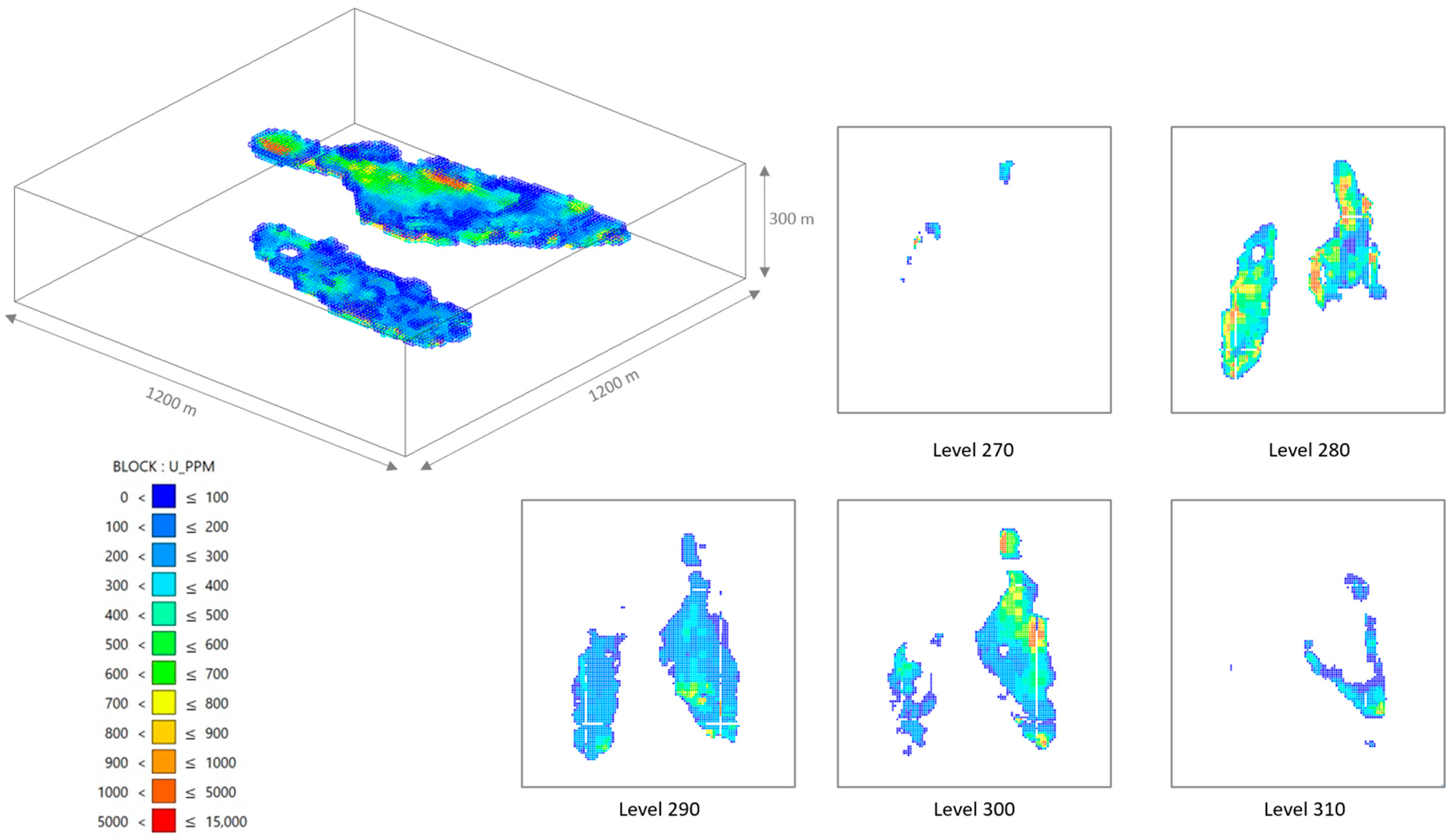
The block model is a general three-dimensional representation of the deposit in small-sized blocks. Each block contains relevant information such as grade, density, and geology, combined with other data such as commodity prices, mining and processing costs, and technical parameters related to mine design [8,27,30]. This study started with the exploration of the block model generated from a database of the project’s boreholes. It consisted of a 1260 m wide, 1330 m long, and 305 m high block model; this large block was subdivided by 35 × 35 × 5 m blocks and smaller 5 × 5 × 2.5 m blocks. Figure 2 shows that the grades ranged from 0 to 15,000 ppm of uranium. Lower grades of blue coloration prevailed from north to south, and higher grades of reddish coloration prevailed in the central zone and north of the northeast body. At depth, the mineralization started at 270 m in a very low percentage and increased up to the 280 m level, where there was important mineralization. Subsequently, the grades decreased in both bodies at the 290 m level, and then, at the 300 m level, the northeastern body had a grade increase, and the southwest geological body disappeared. The northeast body disappeared at the 310 m level. With this information, it was determined that it was necessary to remove 70 m of waste (380–310 m) to reach the mineralization and that the ore body had a thickness of 30 m.

2.2. Economic Block Model

The block economic model was evaluated with the economic parameters shown in

Table 1. Mining and milling costs, prices, and cut-off grade used.

Economic Parameters	Value
Product price (USD/pounds)	95
Mining costs (USD/t)	9
Milling costs (USD/t)	12
Recovery	0.85
Cut-off (ppm)	118

. As mentioned, a mean uranium selling price was considered from the price data of the last 5 decades [26]. Mining costs, processing costs, and the cut-off grade were 2014 values. Regarding metallurgical recovery, a common parameter was considered a product of defined studies.

The key to profitable mining is to consider that revenues are greater than costs, so the combination of these parameters should result in a positive cash flow. These were defined by decisions such as which blocks should be mined, when they should be mined, and whether they should be considered as ore or waste, which depended exclusively on economic parameters [4,31]. It was necessary to estimate the benefit for a Base Case (BC) of a given production value and then for its variations. It was proposed to analyze what would happen if it was decided to decrease or increase the annual production in four scenarios (

Table 2. Annual, daily, and hourly production scenarios.

	Annual Production (t/yr)	Daily Production (t/day)	Hourly Production (t/h)	Comment
Scenario 1	600,000	1644	103	Production decrease
Scenario 2	1,200,000	3288	205	Base Case
Scenario 3	3,000,000	8219	514	Production increase
Scenario 4	6,000,000	16,438	1027	Production increase

The background colour represents each economic scenario.

).

2.3. Nested Pits Definition

Optimizing long-term production scheduling is one of the most important aspects of a mining plan. The objective of long-term production scheduling is to determine the timing and sequence of mining [32]. Additionally, it is necessary to determine the movement of materials, ore, and waste, to maximize profit within existing economic, technical, and environmental constraints [33,34]. The economical block model was used as the input for the optimization process, considering the production for each scenario. The ultimate pit defines what is economically mineable in a deposit, and it was obtained from the Lerchs and Grossmann algorithm [35], which is used in the Maptek’s Pit Optimiser module.

Table 3. Optimization parameters.

Maximum Annual Production Capacity (t/yr)	600,000	1,200,000	3,000,000	6,000,000
Product price (USD/pounds)	95
Selling Costs (USD/pounds)	0
Mining Costs (USD/t)	9
Milling Costs (USD/t)	12
Final Slope Angle (º)	50
Decrements in block value (%)	2
Discount rate (%)	8

The background colour represents each economic scenario.

presents the economic parameters used in the optimization process; in addition to the costs already described, the discount rate is also included, which is one of the parameters of greatest interest when analyzing the feasibility of a project. For this study, a value of 8% was used, which is common in feasibility-level projects [36].

For more information about this algorithm, authors such as Osanloo [7] have made a review of models and algorithms in large-scale optimization. Additionally, Ben-Awuah et al. [33] analyzed some strategic mining optimization options in open pit mining and underground mining, maximizing NPV and comparing results in terms of tons mined and Stripping Ratio (SR). The algorithm evaluates the economic value of each sub-block and parent block, considering the costs required for its extraction and processing, the revenue from its subsequent sale, and the release costs of the associated waste [31]. If this value is positive, it is considered a suitable ore for extraction and processing, and otherwise it will be waste [10].

Within the ultimate pit, the deposit is divided into nested pits ranging from the smallest pit, with the highest value per ton of ore, to the largest pit, with the lowest value per ton of ore [7]. Nested pits have very close boundaries, with minimal tonnage differences from one boundary to another. However, if the orebody grade increases sharply with depth, or the orebody is discontinuous, pushbacks are designed because a significant tonnage difference occurs between the nested pits.

2.4. Phase Sequence

The temporary production scheduling stage depends on the pushbacks, which are a key component for the final design of the mine and the profit obtained. Pushbacks are used as a guide to define the phases, where the extraction process begins, and where it stops. The criteria used for the selection of the phases and the ultimate pit is the determination of the highest NPV values in the best and worst cases [37,38]. First, a normalization of the best and worst cases concerning the highest NPV in each case was performed and then compared to an average of both. In Adiansyah et al. [39], normalization of the data to an ideal value was used to compare and select the most feasible scenario. The percentage differences of NPV for these maximum values were analyzed, and the smallest possible fluctuation concerning the average was chosen. Scenario 4 (Figure 3a) shows that the lowest fluctuation occurred between pits 10 to 23, approximately. Then, Jélvez et al. [34] proposed a methodology for the design of pushbacks, and applied some criteria such as minimization of the SR, minimizing the tons of waste, and maximizing the tons of ore, into pushbacks. Figure 3b shows that the SR increased from Pit-21. Then, Figure 3c shows that the waste was reduced in totality in Pit-23. Finally, considering that the highest NPV with the lowest fluctuation was between Pit-20 and Pit-25, an intermediate Pit-23 was chosen as the ultimate pit. The same criteria were used for the other scenarios.

2.5. Operative Design

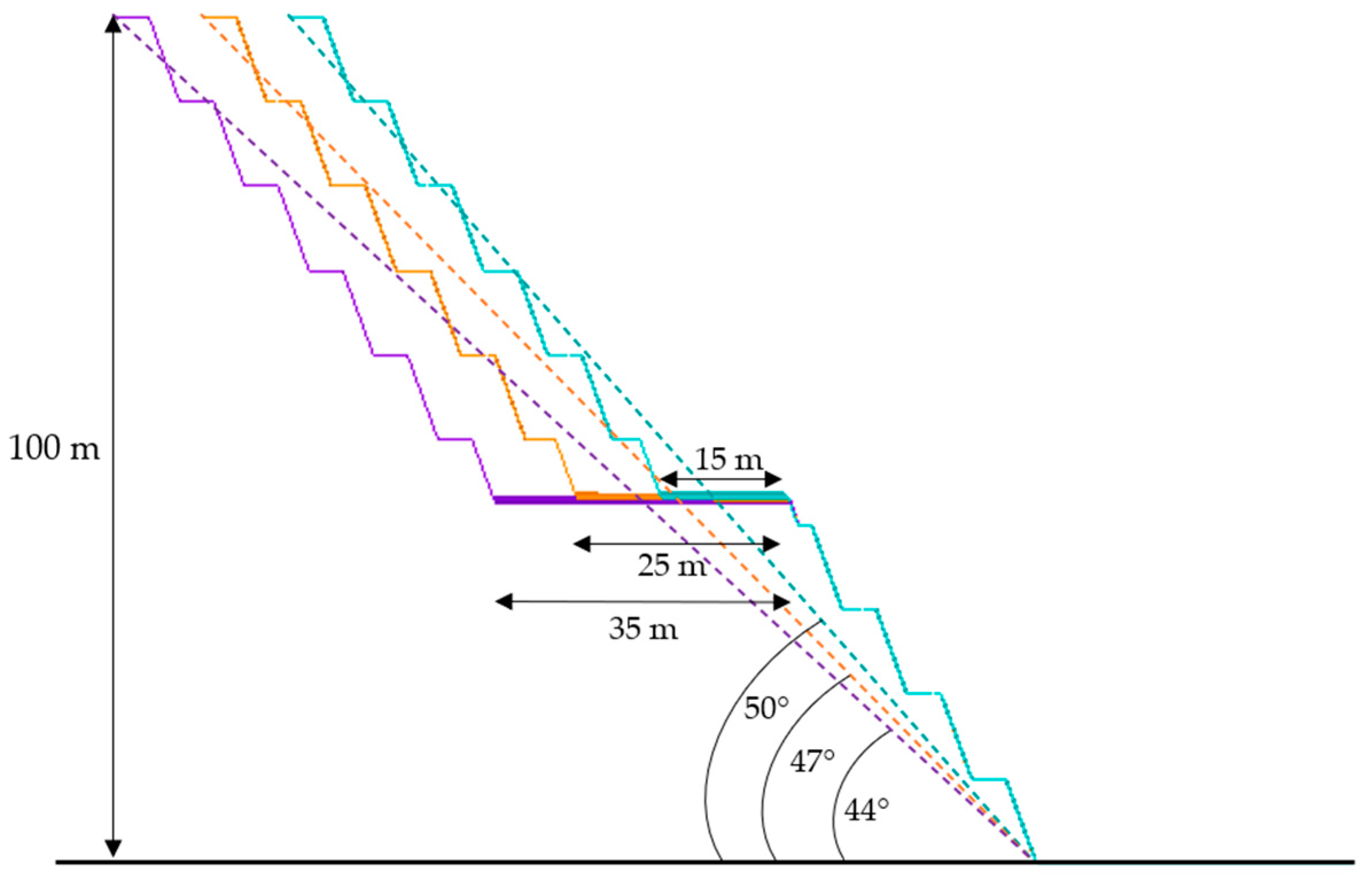
The most relevant geometrical parameters in a ramp were considered for the open pit design (

Table 4. Geometric ramp parameters.

Ramp Width (m)	15	25	35
Final Slope Angle (°)	50	47	44
Ramp Slope (%)	10
Grade Resistance (%)	2
Bench Height (m)	10
Bench Slope (°)	70
Berm Width (m)	4

The background colour represents each design scenario.

). Specifically, ramp width is relevant as it not only has safety implications in terms of vehicle maneuverability and maintaining road continuity [40], but also has significant NPV effects. A variation in the ramp width was used because the final slope angle decreased as this width increased (Figure 4), which implied a greater removal of waste [10,12]. The final slope angles obtained required 9 benches and 9 berms to reach the 100 m slope. In addition, the ramp passed only once over the slope. This ramp considered two lanes, where the width of the roadway must be at least three times the width of the widest vehicle, following the safety specifications in Spain [41]. Other open pit design guidelines mention that aside from the minimum width, additional width should be considered to accommodate equipment larger than the primary road users or to improve sight distance, which should give sufficient space for moving vehicles to avoid collision with stalled or slow-moving vehicles [40].

2.6. Production Scheduling

In the mining plan, the optimization of the production schedule is a crucial step and has an important economic and environmental impact. It has an economic impact because the tons of ore and waste to be extracted are the target of the production optimization, and an environmental impact because the environmental costs should be internalized in this production schedule [42]. One of the most important considerations in this step is the loading and hauling stage, due to the hours that must be invested and the associated costs, both in initial investment and operation. From the performance curves of the selected equipment, available in all manufacturers’ catalogs, the speeds, transport, and cycle times were estimated and, therefore, the productivity of the truck fleet was found for each scenario. Then, with this information, fuel consumption and, therefore, CO₂ emissions could be estimated [14,22].

2.6.1. Equipment Selection

Equipment selection was focused on the transport stage, which required knowledge of daily production, due to the equipment to be considered needing to satisfy the initial production requirement. A first estimate of equipment dimensions was based on the O’Hara formulations [43], which estimated 6–30 tons of capacity for the loaders and 30–90 tons of capacity for the trucks. Loader and truck dimensions were proportional to the tons per day for each of the cases and increased as the tonnage increased. A few catalogs of Caterpillar [44,45,46] were chosen for the selection of the equipment; these catalogs present the characteristics in terms of capacity and dimensions. Three trucks and three loaders were selected, seeking to double the size and capacity of the previous one, to satisfy ramp width and production conditions proposed from a realistic viewpoint, as detailed in

Table 5. Mining truck and wheel specifications.

Ramp Width (m)	Truck Model	Wheel Loader Model	Width Truck (m)	Empty Truck Weight (kg)	Gross Vehicle Weight (kg)	Payload (m3)	Payload (tons)
15	770G	992	4.78	33,224	71,214	17.20	38
25	777G	994	6.10	70,753	163,360	42.00	93
35	789D	998	7.65	141,214	324,319	108.00	183

The background colour represents each design scenario.

.

2.6.2. Haulage Profile

Cycles Times

Following equipment selection, performance was estimated using rimpull curves and retardation curves. These curves are used when the trucks are moving uphill and downhill, respectively, and are especially important to estimate the speed of the truck on a specific route considering parameters such as the Gross Vehicle Weight (GVW) and the Total Resistance (TR), which are given by:

$$\mathrm{GVW}=\mathrm{Empty}\mathrm{truck}\mathrm{weight}+\mathrm{Payload}$$

(1)

$$\mathrm{TR}=\mathrm{Grade}\mathrm{Resistence}\left(\mathrm{GR}\right)+\mathrm{Rolling}\mathrm{Resistence}\left(\mathrm{RR}\right)$$

(2)

where GR is the haul road slope; RR is the force resisting the movement and depends on the tire characteristics and the haul road surface. These parameters allow for determining the traction force (RF), which is the force available between the tire and the ground to propel the machine, according to Soofastaei et al. [15], and is given by:

$$\mathrm{RF}=\mathrm{GVW}\times \mathrm{TR}$$

(3)

When a truck is moving at a constant speed, the rimpull force and velocity can be calculated according to the rimpull–speed–gradeability curve extracted from the manufacturer’s catalog. This is because the engine power is given by the following equation:

$$\mathrm{Engine}\mathrm{Power}=\mathrm{Thrust}\mathrm{Force}\times \mathrm{Speed}$$

(4)

A more detailed description of how the information was extracted from the rimpull curves can be found in each manufacturer’s catalog. Figure 5a shows the information in terms of rimpull and speeds for each selected truck, where logically the larger trucks have greater load capacity, thrust, and higher maximum speeds. One limitation is that all trucks will reach a maximum speed of 50 km/h [41].

Fuel Consumption

Fuel consumption is strongly impacted by factors such as tire usage, age, vehicle maintenance, idling times, engine operating parameters, and transmission shift patterns. In addition, external factors related to weather such as temperature, humidity, wind effects, traffic, and driver behavior are also important [14,22]. Fuel consumption in trucks can be calculated using the following equation [15]:

$$\mathrm{FC}=\frac{\mathrm{SFC}}{\mathrm{FD}}\times \left(\mathrm{LF}\times \mathrm{P}\right)$$

(5)

where SFC is the specific fuel consumption of the engine at maximum power (0.213-0.268 kg/(kg/kW$\times$h)), and FD is the fuel density (0.85 kg/L for diesel). Additionally, the following simplified equation can be used [47]:

$$FC=0.3\times \left(LF\times P\right)$$

(6)

where LF is the engine load factor and is defined as the ratio of the average payload to the maximum load in an operating cycle. At continuous operation using the recommended truck weight, the load factor is 30-40%. P is the truck power (kW). To achieve the best performance of the truck operation, P is determined by:

$$P=\frac{1}{3.6}\times \left(RF\times V_{max}\right)$$

(7)

where RF is the product of the rimpull (R) and the gravity acceleration (g). V_max is the maximum velocity obtained. Figure 5b shows the fuel consumption in two situations: when the truck moves uphill, where fuel consumption is higher because the engine overcomes the gravity force, and when the truck moves downhill, where fuel consumption is minimal since the gravity force acts in the same direction. In addition, this graph shows that fuel consumption in larger trucks is exponentially higher compared to smaller trucks. In general, fuel consumption varies as the truck accelerates and then becomes constant as it increases speed.

This information was the input for the Truck Library of the Haulage Profile tool by Maptek-Vulcan. The cycle estimation and fuel consumption for each ramp were performed using the Route Cycle Estimation tool. Logically, the completely loaded truck would go uphill from the bottom of the pit to the surface; once it has left the material on the surface, without considering transport to the stockpile, the empty truck returns to the bottom. The reason why transport to a stockpile is not considered is that the study intends to analyze the difference in truck consumption, making it unnecessary to consider an additional distance in the estimate. The routes of each ramp contain distance and slope information, and they were created from the pit design in each scenario. These lines were registered in the software with the Build Route Network tool, where the rolling resistance value was also defined. With this tool, you can specify the truck used and the type of material transported for each route (ore or waste). The tool performs a general estimation of speed and fuel consumption for each potential slope (2–16°) and considers each truck’s parameters according to the Truck Library, since it is possible to assign each truck to a route. It then takes the route line and estimates the time required for the trip and fuel consumption, depending on the slope and line distance and on whether the truck is loaded or empty.

Performance

The operating process was adapted using the Time Usage Model [48], commonly applied in the mining industry. This tool allows the identification of efficiency losses through key time usage metrics, or indicators such as the Available Time (AT) and the Utilized Time (UT). The AT represents 80% of the calendar time and comprises the mine scheduled hours, subtracting the downtimes, which include scheduled hours such as holidays or maintenance and unplanned hours caused, for example, by weather conditions. In addition, UT is the scheduled hours of the machine, whose losses are due to shift changes, lunches, and meetings. These hours are the productive hours, the effective time when the machines are in operation, and they represent 75% of the AT. Since this is a relatively small mining operation, two shifts of 8 h per day are considered, displaying the resultant hours in

Table 6. Mining Schedule.

Schedule Parameters	Value
Shift (u)	2
Shift (hours)	8
Working days (days)	365
Calendar time (hours)	5840
Available Time (%)	80
Utilized Time (%)	75

.

The effective capacity of the shovel was estimated, which considered the filling factor, swelling, and density of the material. In addition, instantaneous, operating, and annual performances were obtained. Then, the fleet required to cover the production demand was evaluated. The following formulations were used for this process:

$$EffectiveCapacity=\frac{NominalCapacity\ast FillFactor\times Density}{\left(1+Swelling\right)}$$

(8)

$$InstantaneousPerformance=\frac{EffectiveCapacity}{Cycle}$$

(9)

$$OperationalPerformance=InstantaneousPerformance\times Utilisedtime$$

(10)

$$AnnualPerformance=OperatingPerformance\times Availabletime$$

(11)

$$Units=\frac{AnnualPerformance}{AnnualProduction}$$

(12)

2.6.3. CO₂ Emissions

In the mining process, the loading and hauling stages are the main GHG contributors [21,49]. Trucks use a significant amount of diesel fuel, and this consumption depends on many factors already mentioned [22]. In terms of truck performance, fleets are often heterogeneous regarding fuel consumption and GHG emissions. Optimizing haul operations is key to reducing the environmental footprint in the mining industry [13]. To compare the possible scenarios, the emission factor 2.7 kg CO₂/L fuel was used [21].

3. Results and Discussion

3.1. Net Present Value

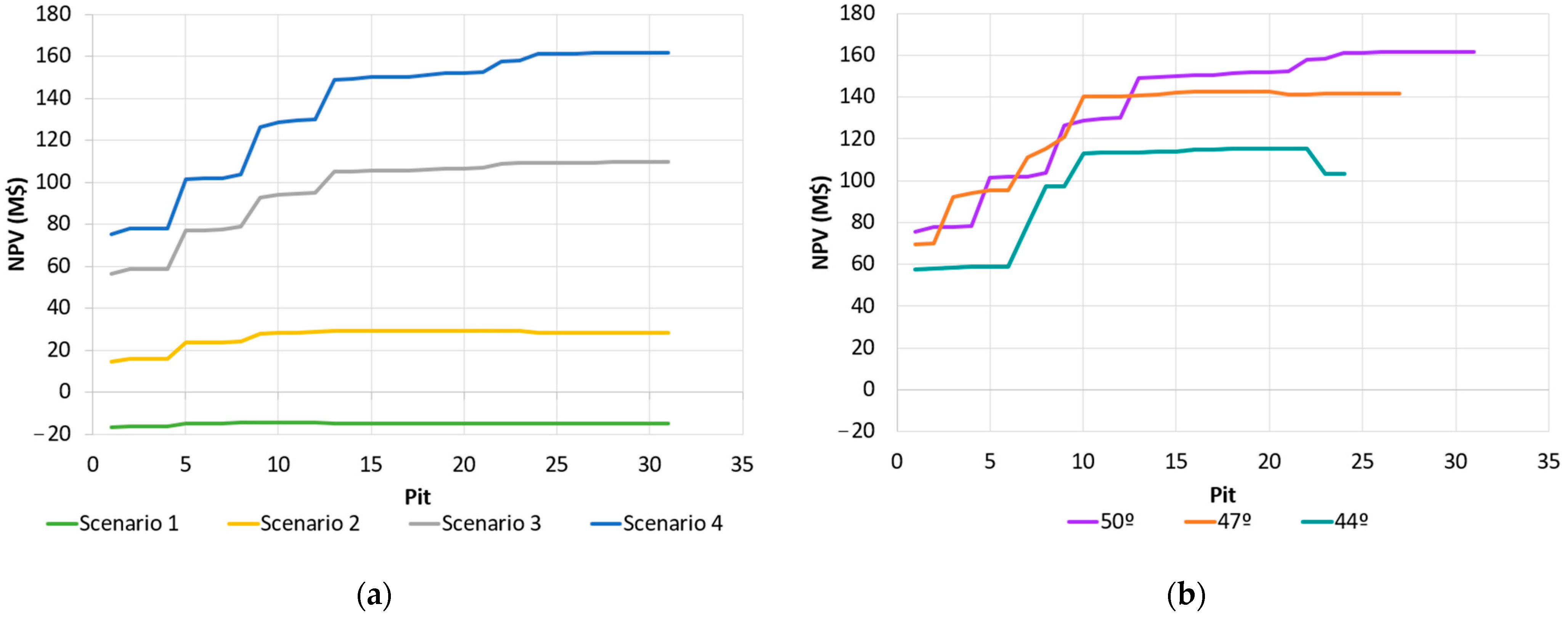
Figure 6a shows the best-case NPVs in the proposed production scenarios. In the lowest production scenario, a negative maximum NPV was observed. This indicated that the proposed production value did not include enough ore to cover operational costs. Then, in the higher production scenarios, NPV was significantly higher because more cash flow was generated as production increased. In addition, lower operating costs generated higher NPVs [16]. Specifically, the NPV would increase significantly if mining costs were lowered, compared to lower processing costs. This is because mining costs affect a larger amount of ore and waste blocks, contrary to milling costs which only affect the blocks considered ore [50]. A similar result is presented in Figure 6b, where the angle of the final pit slope was evaluated. The NPV decreased as the final slope angle decreased, and the ramp width increased. The final slope angle had great sensitivity on the NPV, because the less inclined the final slopes were, the greater the rock extraction on the pit walls, which was reflected in a decrease in profit.

3.2. Ultimate Pit

The ultimate pit was defined for each annual production scenario.

Table 7. Pit Optimizer Results—Scenarios.

	Annual Production (t/yr)	Ultimate Pit	Ore—Best (Mt)	Waste—Best (Mt)	SR (Waste/Ore)	NPV (MUSD)	LOM (yrs)
Scenario 1	600,000	4	3.12	11.39	3.65	(16.08)	24.18
Scenario 2	1,200,000	8	3.91	16.36	4.18	24.30	16.89
Scenario 3	3,000,000	14	8.58	31.13	3.63	105.15	13.24
Scenario 4	6,000,000	23	10.49	40.55	3.86	158.17	8.51

The background colour represents each design scenario.

shows the clear difference between mined tons of ore. The constraint of low annual production, which does not cover operating costs, resulted in unprofitable mining. Additionally, the SR could be obtained; this value varied from 3:1 to 4:1, which assumes economic viability in higher production cases because NPVs increase exponentially. It is evident that as annual production increased, the ultimate pit deepened and the LOM decreased, thus decreasing operating expenses and increasing the NPV by having a higher cash flow each year, although the SR was maintained. On the other hand,

Table 8. Pit Optimizer Results—Slope Angle Variation.

	Ramp Width (m)	Final Slope Angle	Ultimate Pit	Ore—Best (Mt)	Waste—Best (Mt)	SR (Waste/ Ore)	NPV (M USD)	LOM (yrs)
Scenario 4	15	50	23	10.50	40.55	3.86	158.17	8.51
	25	47	20	8.88	33.42	3.76	142.68	7.05
	35	44	15	8.74	35.06	4.01	113.71	7.30

The background colour represents each design scenario.

presents the same variables for the ramp width variation or final slope angle in Scenario 4. In general terms, this angle had a direct impact on SR since as it decreased waste extraction increased, and therefore the NPV decreased. Specifically, the expansion of the last pit was limited by the widening of the ramp, so that the mined ore and waste tons decreased. However, this variation of Scenario 4 was better than the lower production scenarios.

3.3. Pit Design

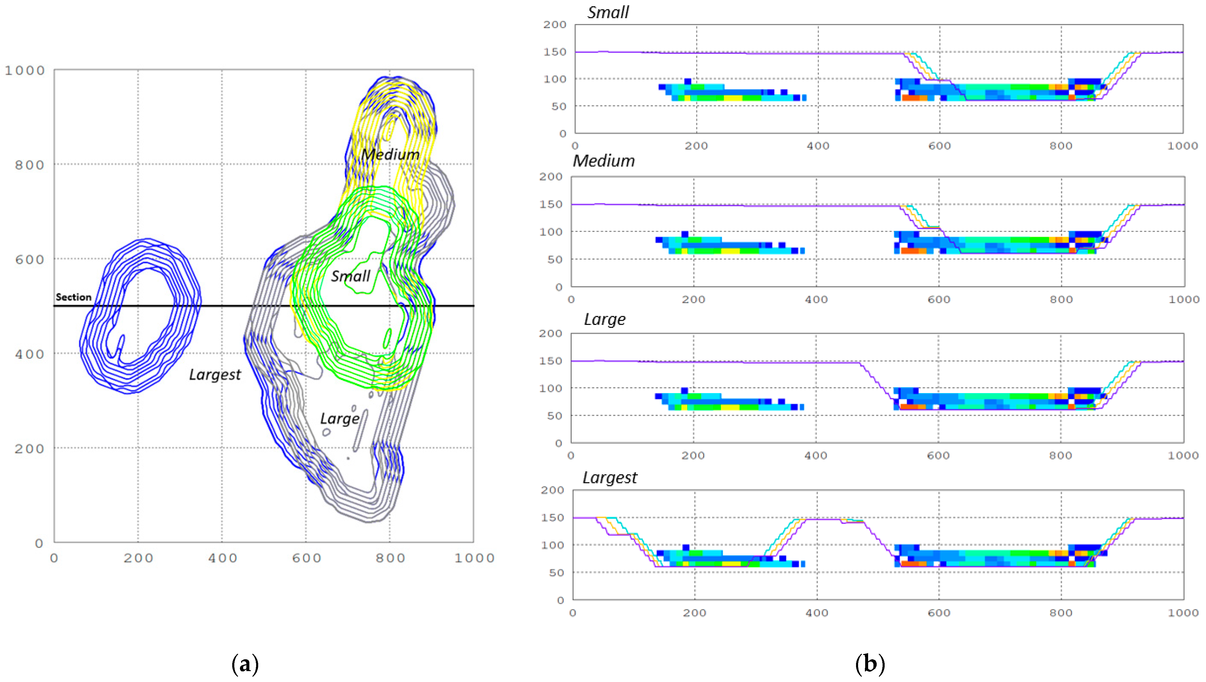
The production scenarios’ variation showed that nested pit geometry does not change significantly. In other words, for any economic scenario, the final pit geometry was maintained, in general terms, and the most important aspect that varied was the mining speed and, therefore, the LOM. The reason for this was that the grades and geometry of the deposit were fixed and do not change. Therefore, the optimization algorithm, as well as the pit design, tried to match the initial bench feet with the richest mineralization and continue into the best-mineralized zones. Only Scenario 4 reached the richest and deepest mineralized zones and the second geological body, so choosing the right production scenario is key to the correct and complete extraction of the resources. Then, the analysis was transferred to a rather geometrical sense, considering pit dimensions or scales. Figure 7 illustrates, in a plan view and profiles, the final pits according to the Pit Optimizer tool. Sections show that the final pits expanded horizontally, reaching the same depth either by varying the annual production or by varying the ramp width. The final pit dimensions, according to their scale, were named Small (Pit-4), Medium (Pit-8), Large (Pit-13), and Largest Pit (Pit-23).

The scenario matrix (Figure 8) was obtained by combining the geometries of the annual production scenarios with the ramp width variation, which considered the pit dimensions according to annual production on the horizontal axis, from a “small pit” to a “largest pit”, and the mining design from a 15 to a 35 m ramp. The pit designs changed minimally as the ramps became wider. This was because it is difficult to give continuity to a wider ramp, due to it being necessary to smooth the curves for the ramp to fit correctly. In addition, it was observed that the final lengths did not vary when the ramp width varied.

3.4. Hauling

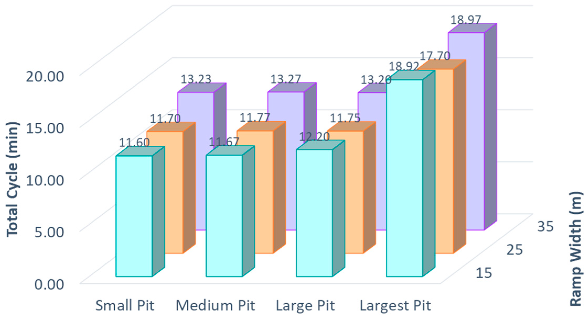
The total cycle estimation (loading time + transport time) of the scenario matrix (Figure 9) was obtained using the speed information according to the rimpull’s truck, considering the truck’s maximum load, ramp slope, and minutes required in each loading stage. For the small, medium, and large pits, there were no significant changes since the equipment maintained a similar range of maximum speeds and the final distances did not vary much. However, there was an increase in the cycle time in the largest pit (30–36%), and this is quite logical because when contemplating another geological body, haulage distances and transport times would increase. The fact is that these distances would be affected if it was decided to vary the slope of the ramp. If the ramp slope was increased, the distances would be shortened, but trucks will not necessarily get there faster, since the speed would decrease [22]. Another important fact that has not been considered is the time required by trucks to arrive at a stockpile or dump site, where the destination site could be further away. Therefore, the cycle could be considerably higher, especially in large pits.

3.5. Production

From the effective capacities of the shovels and each associated truck, combined with the cycle time, it was possible to calculate the truck performance for each economic scenario. Despite having a similar total cycle time, the best indicator was the operational performance or operational output (Figure 10a). Small trucks have lower productivity than large trucks, and as the pit dimensions increased, the productivity of the same truck decreased due to the increase in the transport cycle; therefore, for the same truck in a larger pit, productivity decreased significantly. A loss of productivity in large trucks is more frequent than in small trucks, so the availability or utilization of this equipment must be increased, which is difficult since equipment maintenance is more complex [12]. The truck units are presented in Figure 10b, where it can be seen that productivity loss in large trucks is more frequent than in small trucks, so it is necessary to increase the availability or utilization of this equipment, which is difficult since their maintenance is more complex [12]. In the small and medium pits, the small truck would be ideal and the medium and large trucks are oversized. In the largest pit, using large trucks, the number of units needed decreases by 80% concerning small trucks, while NPV decreases by 30%.

3.6. Fuel Consumption

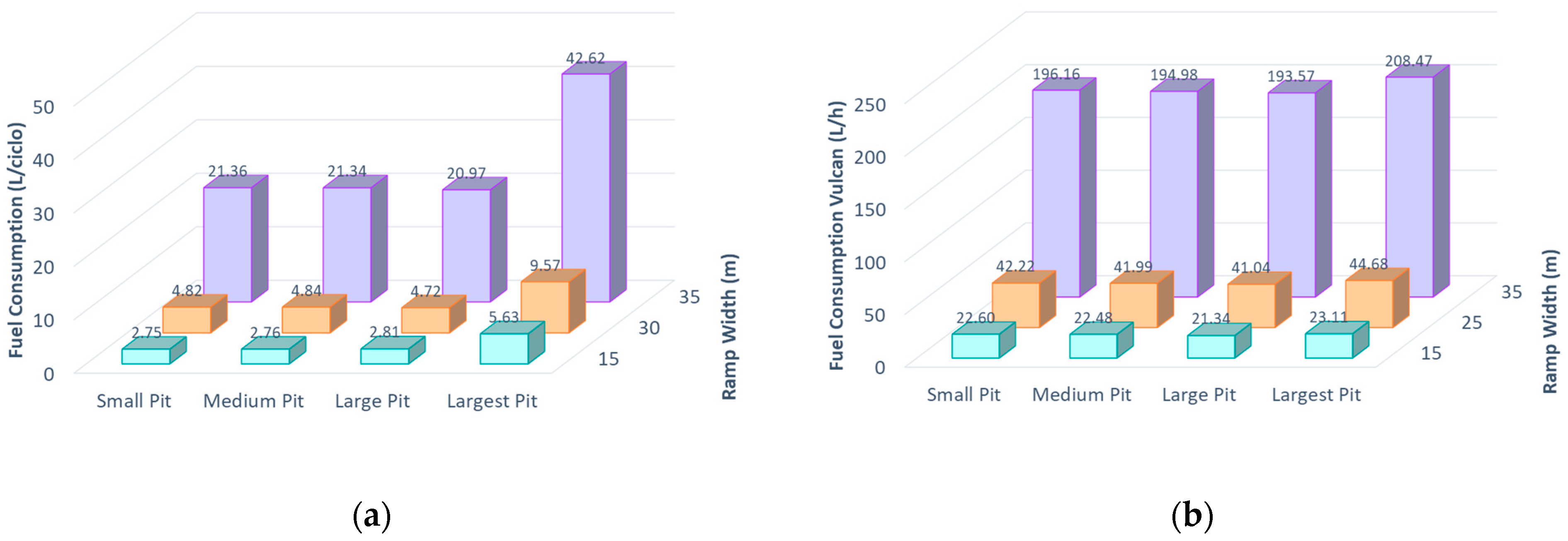
Figure 11a shows the data obtained from the fuel consumption per cycle of the scenario matrix. Despite the same distances and almost similar times, the fuel consumption was higher in the larger trucks, assuming an increase of up to 300% compared to the medium truck scenario and in contrast to the decrease of up to 40% in smaller trucks. Combining these data with the cycle time, Figure 11b shows the fuel consumption per hour of the scenario matrix. These data were compared with the average consumption of Caterpillar’s Catalog, (2015), obtaining values in line with their normal average consumption.

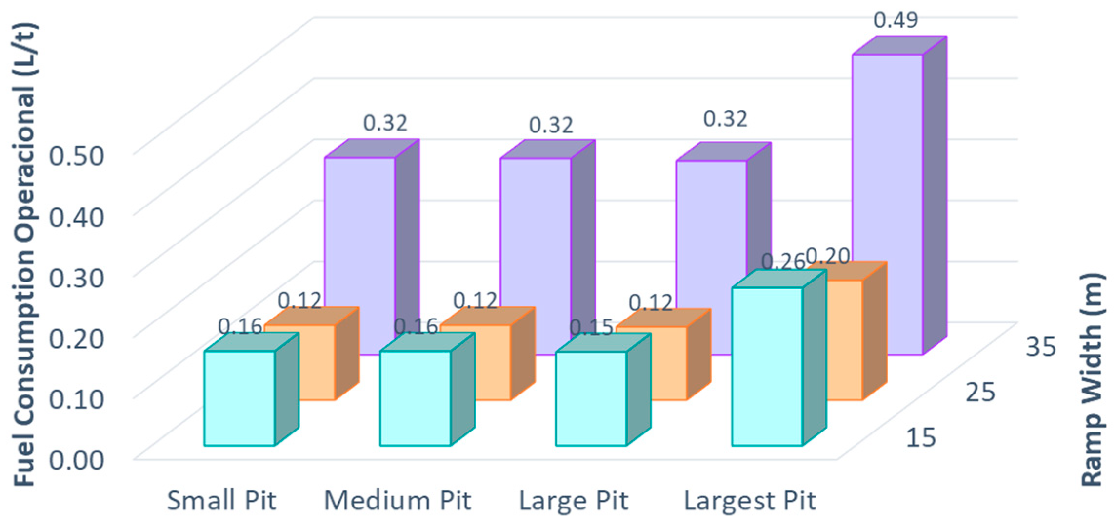
Considering the great importance of these parameters in decisions such as the purchase of equipment in a mining project, this type of analysis should be carried out preliminarily, considering equipment availability, prices, road characteristics, regulations according to the current laws of the site, and the environmental impact. The uncertainty lies in whether it is necessary to purchase more units of equipment to meet production targets or whether the environmental cost of large equipment in terms of fuel consumption, with the associated emissions, must also play a role in the decision-making from a holistic perspective. Subsequently, Figure 12 shows the ratio between fuel consumption (liters/hour) and operational productivity (t/h). This ratio allows for a deeper understanding of energy consumption. Fuel consumption per ton doubled in larger trucks and as the pit size increased. In other words, the environmental cost per ton mined doubles when larger trucks are used.

3.7. Environmental Impact Related to the Operation Process

Figure 13a shows CO₂ emissions per liter of fuel consumed. As expected, there was a higher consumption of larger equipment and, therefore, higher emissions. In the same way, CO₂ emissions were compared with respect to annual tons produced and, as can be seen in Figure 10b, the ratio increased considerably in small trucks. In addition, having more units in small trucks would increase the supply consumption for the maintenance and emission of particles on unpaved roads, by stockpiles and others [21].

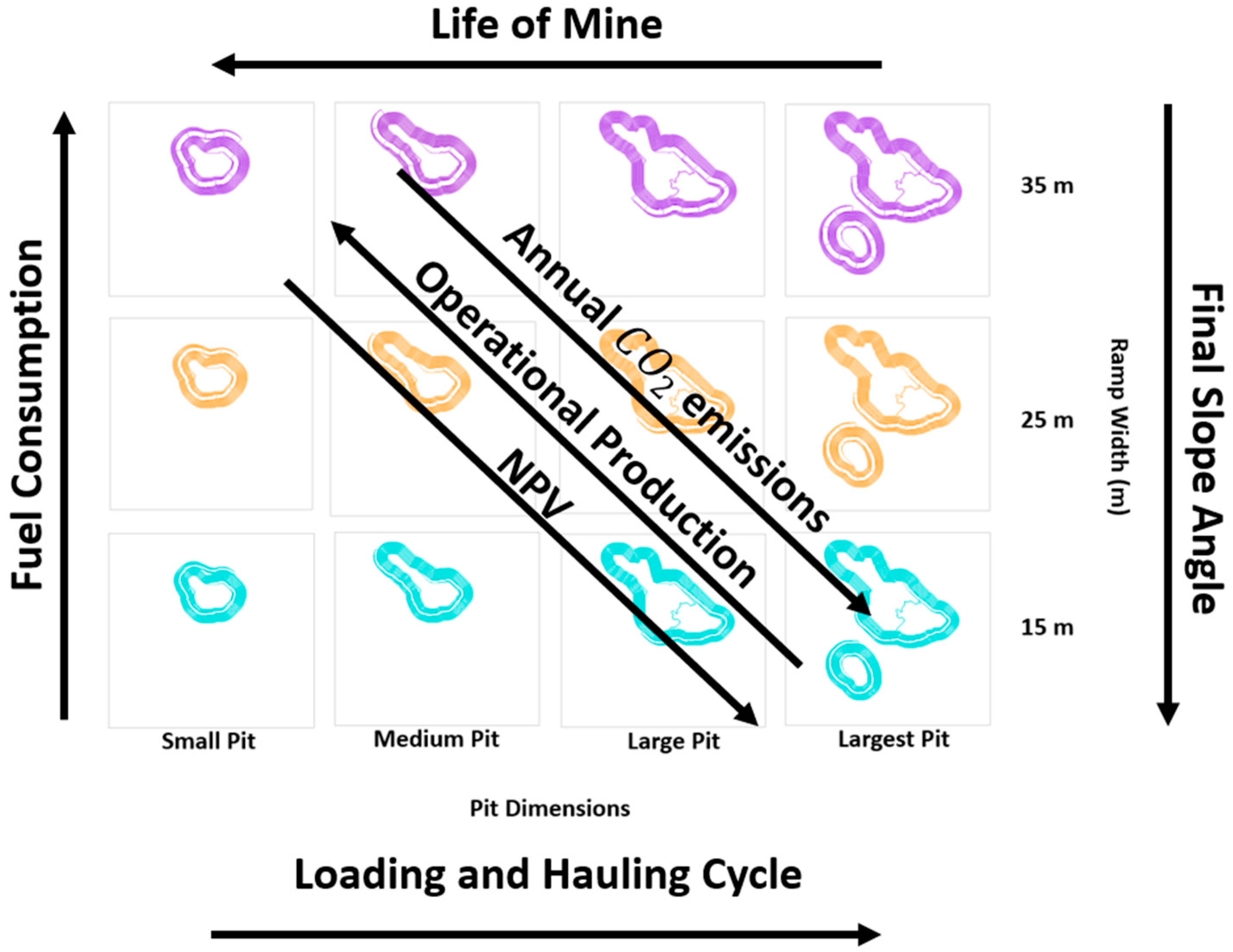
Results are summarized through the scenario matrix detailed in Figure 14. This figure shows that annual production interacted with mine design and mine planning, directly affecting NPV. This annual production determined the final value of the project and LOM, and increasing annual production increased NPV and decreased LOM significantly. Despite the variations in the parameters, following the same conditions, the geometry of the final pits was the same, and what varied was the rate of extraction of the blocks and, therefore, the NPV. As for the technical parameters, the final pit slope angle was evaluated, which had a direct correlation with the width of the ramp because, as the width of the ramp increased, the angle of the final slope decreased. The final slope angle had a high sensitivity on NPV, since it decreased as final slope steepness decreased and increased waste rock removal from the pit walls.

The variation in ramp width was evaluated with equipment selection. It should be taken into account that the LOM should coincide with the useful life of the equipment (not specified in this work), so if the annual production is increased and large trucks are used, LOM is shortened, and the initial investment could be unnecessary.

Despite having similar hauling distances, the speed and fuel consumption in the loading and hauling stages differed more visibly. It was found that the difference was because larger vehicles tend to be faster, and operational productivity is considerably higher in larger equipment. However, fuel consumption doubles in the larger trucks, but results showed that annual CO₂ emissions were higher when using smaller trucks.

4. Conclusions

The combination of different scenarios and designs was used to evaluate options in mining project decisions. These options made it possible not to overestimate or underestimate the choice of important variables such as annual production or equipment size. Additionally, these options need to consider ESG indicators such as the environmental impact of CO₂ emissions. This study indicates that achieving high operational production with the minimum possible equipment is not necessarily the best option.

On the one hand, the use of large trucks implies a wider ramp, and this has a big impact on the ultimate pit. In terms of SR, concerning the medium scenario, it increases by 7% for large trucks and only 3% for small trucks. This variation has a direct impact on the economics of the project, as the NPV decreases by 20% for large trucks, but increases by 11% for small trucks, compared to the same medium scenario.

On the other hand, using small trucks generates a longer fleet size, and concerning the medium scenario can result in a 150% increment in the number of units of equipment needed, which will require an initial investment for the purchase of equipment and many personnel in the long term. In contrast, with the use of large trucks, a 30% reduction of units can be achieved, although it should be considered that more specialized labor is needed and that regulations are more stringent. Many mining projects, because of limited investment or high investment risk, choose to apply a sequential mining system in the purchase of small trucks at the beginning of mining.

In terms of environmental costs, CO₂ emissions per liter of fuel increased by 7–30% in small trucks concerning the medium scenario, while in large trucks these emissions increased by 200–300%. When the same comparison was made from an annual compendium of emissions per mined ton, in small trucks there was an increase of up to 200% concerning the medium scenario, while in large trucks it was only 56% for the largest pit.

References

1. Newman, A.M.; Rubio, E.; Caro, R.; Weintraub, A.; Eurek, K. A Review of Operations Research in Mine Planning. Interfaces 2010, 40, 222–245. [Google Scholar] [CrossRef]
2. Nicolet, J.P. Methods of Exploitation of Different Types of Uranium Deposits; Nuclear Fuel Cycle and Materials Section; International Atomic Energy Agency: Vienna, Austria, 2000. [Google Scholar]
3. Askari-Nasab, H.; Frimpong, S.; Szymanski, J. Modelling Open Pit Dynamics Using Discrete Simulation. Int. J. Min. Reclam. Environ. 2007, 21, 35–49. [Google Scholar] [CrossRef]
4. Hustrulid, W.; Kuchta, M.; Martin, R. Open Pit Mine Planning and Design; CRC Press/Balkema: London, UK, 2013; Volume 1, ISBN 978-1-4665-7512-7. [Google Scholar]
5. Sanmiquel, L.; Bascompta, M.; Rossell, J.; Anticoi, H.; Guash, E. Analysis of Occupational Accidents in Underground and Surface Mining in Spain Using Data-Mining Techniques. Int. J. Environ. Res. Public Health 2018, 15, 462. [Google Scholar] [CrossRef] [PubMed]
6. Tsopa, V.; Cheberiachko, S.; Yavorska, O.; Deryugin, O.; Bas, I. Increasing the Safety of the Transport Process by Minimizing the Professional Risk of a Dump Truck Driver. Min. Miner. Depos. 2022, 16, 101–108. [Google Scholar] [CrossRef]
7. Osanloo, M.; Gholamnejad, J.; Karimi, B. Long-Term Open Pit Mine Production Planning: A Review of Models and Algorithms. Int. J. Min. Reclam. Environ. 2008, 22, 3–35. [Google Scholar] [CrossRef]
8. Jara, R.M.; Couble, A.; Emery, X.; Magri, E.J.; Ortiz, J.M. Block Size Selection and Its Impact on Open-Pit Design and Mine Planning. J. South Afr. Inst. Min. Metall. 2006, 106, 205–212. [Google Scholar]
9. Meneses, D.; Sepúlveda, F.D. Modeling Productivity Reduction and Fuel Consumption in Open-Pit Mining Trucks by Considering the Temporary Deterioration of Mining Roads through Discrete-Event Simulation. Mining 2023, 3, 96–105. [Google Scholar] [CrossRef]
10. Diddens, Z.M. Integration of Fleet Production and Cost Analysis in Mine Design and Planning. Master’s Thesis, Delft University of Technology, Delft, The Netherlands, 2019. [Google Scholar]
11. Bozorgebrahimi, E. The Evaluation of Haulage Truck Size Effects on Open Pit Mining; The University of British Columbia: Vancouver, BC, Canada, 2004. [Google Scholar]
12. Bozorgebrahimi, E.; Hall, R.A.; Blackwell, G.H. Sizing Equipment for Open Pit Mining—A Review of Critical Parameters. Min. Technol. (Trans. Inst. Min. Metall. A) 2003, 112, 171–179. [Google Scholar] [CrossRef]
13. Nakousi, C.; Pascual, R.; Anani, A.; Kristjanpoller, F.; Lillo, P. An Asset-Management Oriented Methodology for Mine Haul-Fleet Usage Scheduling. Reliab. Eng. Syst. Saf. 2018, 180, 336–344. [Google Scholar] [CrossRef]
14. Golbasi, O.; Kina, E. Haul Truck Fuel Consumption Modeling under Random Operating Conditions: A Case Study. Transp. Res. Part D Transp. Environ. 2022, 102, 103135. [Google Scholar] [CrossRef]
15. Soofastaei, A.; Aminossadati, S.M.; Arefi, M.M.; Kizil, M.S. Development of a Multi-Layer Perceptron Artificial Neural Network Model to Determine Haul Trucks Energy Consumption. Int. J. Min. Sci. Technol. 2016, 26, 285–293. [Google Scholar] [CrossRef]
16. Ebrahimi, A. Ultimate Pit Size Selection, Where Is the Optimum Point? In Proceedings of the IMCET 2019— 26th International Mining Congress and Exhibition of Turkey, Antalya, Turkey, 16–19 April 2019; pp. 638–645. [Google Scholar]
17. Baek, J.; Choi, Y. A New Method for Haul Road Design in Open-Pit Mines to Support Efficient Truck Haulage Operations. Appl. Sci. 2017, 7, 747. [Google Scholar] [CrossRef]
18. Peralta, S.; Sasmito, A.P.; Kumral, M. Reliability Effect on Energy Consumption and Greenhouse Gas Emissions of Mining Hauling Fleet towards Sustainable Mining. J. Sustain. Min. 2016, 15, 85–94. [Google Scholar] [CrossRef]
19. Kofanov, O.; Vasylkevych, O.; Kofanova, O.; Zozul’ov, O.; Kholkovsky, Y.; Khrutba, V.; Borysov, O.; Bobryshov, O. Mitigation of the Environmental Risks Resulting from Diesel Vehicle Operation at the Mining Industry Enterprises. Min. Miner. Depos. 2020, 14, 110–118. [Google Scholar] [CrossRef]
20. Bascetin, A.; Adiguzel, D.; Tuylu, S. The Investigation of CO2 Emissions for Different Rock Units in the Production of Aggregate. Environ. Earth Sci. 2017, 76, 279. [Google Scholar] [CrossRef]
21. Bascompta, M.; Sanmiquel, L.; Gangolells, M.; Sidki, N. LCA Analysis and Comparison in Quarrying: Drill and Blast vs Mechanical Extraction. J. Clean. Prod. 2022, 369, 133042. [Google Scholar] [CrossRef]
22. Fortescue Metals Group Ltd.; Downer EDII Mining Pty Ltd. Analyses of Diesel Use for Mine Haul and Transport Operations; Department of Resources Energy and Tourism: Canberra, Australia, 2008; pp. 1–18. [Google Scholar]
23. Muñoz, J.I.; Guzmán, R.R.; Botín, J.A. Development of a Methodology That Integrates Environmental and Social Attributes in the Ore Resource Evaluation and Mine Planning. IJMME 2014, 5, 38–58. [Google Scholar] [CrossRef]
24. Soberón Bravo, E. Governance on Lithium Mining Shareholdings: Expanding Environment, Social and Governance (ESG) Indicators to Economic Regulation and Raw Material Politics. Miner. Econ. 2022, 36, 333–3475. [Google Scholar] [CrossRef]
25. Lokuwaduge, C.S.D.S.; Heenetigala, K. Integrating Environmental, Social and Governance (ESG) Disclosure for a Sustainable Development: An Australian Study: ESG Disclosure in Australian De Silva Lokuwaduge and Heenetigala. Bus. Strat. Env. 2017, 26, 438–450. [Google Scholar] [CrossRef]
26. Yellow Cake PLC Pure Exposure to the Uranium Commodity Investor Presentation November 2020. Available online: https://www.yellowcakeplc.com (accessed on 10 March 2023).
27. Morales, N.; Seguel, S.; Cáceres, A.; Jélvez, E.; Alarcón, M. Incorporation of Geometallurgical Attributes and Geological Uncertainty into Long-Term Open-Pit Mine Planning. Minerals 2019, 9, 108. [Google Scholar] [CrossRef]
28. Tolwinski, B.; Newton, M.; Lapworth, A.; Morrison, J. NPV Scheduler: Open Pit Planning: From Geological Model to Optimized Strategic Mine Plan; Datamine Group: Docklands, Australia, 2007. [Google Scholar]
29. Heidari, S.M. Quantification of Geological Uncertainty and Mine Planning Risk Using Metric Spaces. Ph.D. Thesis, University of New South Wales, Sydney, Australia, 2015. [Google Scholar]
30. Rossi, M.E.; Deutsch, C.V. Mineral Resource Estimation; Springer: Berlin/Heidelberg, Germany, 2014; ISBN 978-85-7811-079-6. [Google Scholar]
31. Dagdelen, K. Open Pit Optimisation—Strategies for Improving Economics of Mining Projects through Mine Planning. In Proceedings of the IMCET2001—17* International 17th Mining Congress and Exhibition of Turkey, Istanbul, Turkey, 17–21 September 2001; pp. 145–148. [Google Scholar]
32. Whittle, J. The Facts and Fallacies of Open Pit Optimization; Whittle Programming Pty Ltd.: North Balwyn, Australia, 1989. [Google Scholar]
33. Ben-Awuah, E.; Richter, O.; Elkington, T.; Pourrahimian, Y. Strategic Mining Options Optimization: Open Pit Mining, Underground Mining or Both. Int. J. Min. Sci. Technol. 2016, 26, 1065–1071. [Google Scholar] [CrossRef]
34. Jélvez, E.; Morales, N.; Askari-Nasab, H. A New Model for Automated Pushback Selection. Comput. Oper. Res. 2020, 115, 104456. [Google Scholar] [CrossRef]
35. Lerchs, H.; Grossmann, I. Optimum Design of Open-Pit Mines. Trans CIM 1965, 68, 17–24. [Google Scholar]
36. Taheri, M.; Irannajad, M.; Ataee-pour, M. Risk-Adjusted Discount Rate Estimation for Evaluating Mining Projects. J. Secur. Inst. Aust. 2009, 4, 36–42. [Google Scholar]
37. Bastante, F.G.; Taboada, J.; Ordónez, C. Design and Planning for Slate Mining Using Optimisation Algorithms. Eng. Geol. 2004, 73, 93–103. [Google Scholar] [CrossRef]
38. Lane, K.F. The Economic Definition of Ore; COMET Strategy Pty Ltd.: Cleveland, Australia, 2015; ISBN 978-0-9941852-2-8. [Google Scholar]
39. Adiansyah, J.S.; Rosano, M.; Biswas, W.; Haque, N. Life Cycle Cost Estimation and Environmental Valuation of Coal Mine Tailings Management. J. Sustain. Min. 2017, 16, 114–125. [Google Scholar] [CrossRef]
40. Tannant, D.D.; Regensburg, B. Guidelines for Mine Haul Road Design; University of British Columbia: Kelowna, Canada, 2001. [Google Scholar]
41. Ministry of Industry and Energy. Reglamento General de Normas Básicas de Seguridad Minera. In Boletin Oficial del Estado; Real Decreto 863/1985; Ministerio de Industria y Energía: Madrid, Spain, 1990; Volume 103, pp. 17869–17877. [Google Scholar]
42. Xu, X.; Gu, X.; Wang, Q.; Gao, X.; Liu, J.; Wang, Z.; Wang, X. Production Scheduling Optimization Considering Ecological Costs for Open Pit Metal Mines. J. Clean. Prod. 2018, 180, 210–221. [Google Scholar] [CrossRef]
43. O’Hara, T.A.; Suboleski, S.C. Costs and Cost Estimation. SME Min. Eng. Handb. 1992, 1, 405–424. [Google Scholar]
44. Caterpillar. Surface Mining Primary Loading Tool: Selection Guide; Caterpillar: Irving, TX, USA, 2013. [Google Scholar]
45. Caterpillar. 770G Off-Highway Truck Engine; Caterpillar: Irving, TX, USA, 2014. [Google Scholar]
46. Caterpillar. Caterpillar Performance Handbook; Caterpillar: Irving, TX, USA, 2019; p. 2264. [Google Scholar]
47. Runge, I.C. Mining Economics and Strategy; Society for Mining, Metallurgy and Exploration, Inc.: Englewood, CO, USA, 2009. [Google Scholar]
48. Dzakpata, I.; Knights, P.; Kizil, M.S.; Nehring, M.; Aminossadati, S.M. Truck and shovel versus in-pit conveyor systems: A comparison of the valuable operating time. In Proceedings of the 16th Coal Operators’ Conference, Wollongong, Australia, 10–12 February 2016; University of Wollongong: Wollongong, Australia, 2016; pp. 463–476. [Google Scholar]
49. Norgate, T.; Haque, N. Energy and Greenhouse Gas Impacts of Mining and Mineral Processing Operations. J. Clean. Prod. 2010, 18, 266–274. [Google Scholar] [CrossRef]
50. Anas, A.V.; Amalia, R.; Qaidahiyani, N.F.; Djamaluddin; Herin, S.R.D. Sensitivity Analysis of Net Present Value Due to Optimal Pit Limit in PT Ceria Nugraha Indotama, Kolaka Regency, Southeast Sulawesi Province. In Proceedings of the IOP Conference Series: Materials Science and Engineering, Chennai, India, 16–17 September 2020; Volume 875, pp. 1–11. [Google Scholar]
Figure 1. (a) Traditional methodology for long-term open-pit mine planning. (b) Correlation methodology for scenarios matrix. The phase sequence is defined as scenarios and ramp variations in the operative design.
Applsci 13 05769 g001
Figure 2. Case study block model and depth sections.
Applsci 13 05769 g002
Figure 3. (a) Percentage difference of NPV; (b) stripping ratio; (c) tons of waste to remove in Scenario 4.
Applsci 13 05769 g003
Figure 4. Ramp width effect on final slope angle.
Applsci 13 05769 g004
Figure 5. (a) Maximum speeds; (b) fuel consumption of the selected trucks.
Applsci 13 05769 g005
Figure 6. (a) NPV based on annual production variation; (b) NPV based on the variation of the final slope angle in Scenario 4.
Applsci 13 05769 g006
Figure 7. (a) Plan view; (b) ultimate pit sections of scenarios.
Applsci 13 05769 g007
Figure 8. Scenario matrix: pit dimensions and ramp width variations.
Applsci 13 05769 g008
Figure 9. Scenario Matrix: Cycle.
Applsci 13 05769 g009
Figure 10. (a) Scenario matrix—operational production. (b) Truck units.
Applsci 13 05769 g010
Figure 11. (a) Fuel consumption per cycle; (b) fuel consumption per hour of the scenario matrix.
Applsci 13 05769 g011
Figure 12. Scenario matrix—fuel consumption per ton.
Applsci 13 05769 g012
Figure 13. (a) A) CO 2 emissions per liter; (b) annual CO 2 emissions per Mt of the scenario matrix.
Applsci 13 05769 g013
Figure 14. Scenario matrix tends.
Applsci 13 05769 g014