Abstract
The paper discusses the application of a motion profile with an elliptic jerk to Cartesian space position control of serial robots. This motion profile is obtained by means of a kinematic approach, starting from the jerk profile and then calculating acceleration, velocity and position by successive integrations. Until now, this profile has been compared to other motion laws (trapezoidal velocity, trapezoidal acceleration, cycloidal, sinusoidal jerk, modified sinusoidal jerk) considering single-input single-output systems. In this work, the comparison is extended to nonlinear multi-input multi-output systems, investigating the application to Cartesian space position control of serial robots. As case study, a 4-DOF SCARA-like architecture with elastic balancing is considered; both an integer-order and a fractional-order controller are applied. Multibody simulation results show that, independently of the controller, the behavior of the robot using the elliptic jerk profile is similar to the case of adopting the sinusoidal jerk and modified sinusoidal jerk laws, but with a slight reduction in the position error (−3.8% with respect to the sinusoidal jerk law and −0.8% with respect to the modified sinusoidal jerk law in terms of Integral Square Error) and of the control effort (−8.2% with respect to the sinusoidal jerk law and −1.3% with respect to the modified sinusoidal jerk law in terms of Integral Control Effort).
1. Introduction
The performance assessment of production systems, mechatronic devices and industrial manipulators is a very complex issue, which involves and orients many different design stages: analytical and computer-aided mechanical synthesis [1,2,3], control system design [4], and motion planning [5]. In many robotic tasks the free motion time, without forces exchanged with the environment, represents a significant part or even the whole of the cycle time. Examples are pick-and-place, varnishing and laser welding tasks. Consequently, the definition of innovative profiles for free motion is a motivating and useful research area, since it can improve the system performance in a wide variety of automation applications. Depending on the specific task requirements, different benefits can be pursued, for example, cycle time reduction, energy saving, and residual vibration lessening.
The motion profile of a dynamic system can be defined using dynamic or kinematic approaches. The first class of methods exploits the dynamic model of the system, and the motion profile is optimized while respecting kinematic and dynamic constraints, such as limits on the actuation force/torque, on the acceleration and on the jerk [5,6]. On the contrary, kinematic methods do not utilize the system dynamic model, and the motion profile synthesis is purely kinematics, usually with assumptions and constraints in terms of acceleration and jerk [5,7]. Kinematic methods are undoubtedly simpler, and therefore, they are very widespread in industrial applications, even if the achievable performance is only sub-optimal.
Besides their simplicity, the scientific interest about kinematic methods has another motivation: in the case of repetitive tasks the robot motion can be optimized offline to maximize a specific performance index by dynamic methods. On the other hand, in some cases, it is not possible to optimize the robot motion offline, since the trajectory must be replanned depending on external events, not predictable a priori. An example, with growing industrial importance, is collaborative robotics, in which the robot must modify its trajectory when a human operator enters its workspace [8].
In these cases, the robot motion must be quickly replanned online without time-expensive optimization techniques, but adopting predefined motion profiles. Commonly, to avoid collisions with obstacles, the robot trajectory must be controlled in the Cartesian space of the end-effector external coordinates.
In this paper, a recently proposed motion profile with elliptic jerk [9] is compared to other profiles discussed in the scientific literature with reference to the position control of robots. In [9,10] the elliptic jerk profile has been discussed with application to single-input single-output (SISO) systems. In this work, the investigation is extended to a multi-input multi-output (MIMO) system, a serial robot with Cartesian space position control.
As a case study, the SCARA-like RRFbR robot (Revolute, Revolute, Four-bar, Revolute) with elastic balancing is considered [11]. As regards the algorithm for Cartesian space position control, both an integer-order (IO) and a fractional-order (FO) scheme have been taken into account. Classical Cartesian space controllers (KD) are IO, with a stiffness matrix K that defines the end-effector stiffness in the external coordinates, and a damping matrix D which expresses the end-effector damping, related to the first-order derivatives of the end-effector coordinate errors. Consequently, the KD Cartesian space position control represents a MIMO extension of the PD control for SISO systems, in which there is a term P proportional to the error and a term D proportional to the first-order derivative of the error.
A possible FO extension of the KD controller is represented by the KDHD controller [12], in which a damping of order 1/2 (half-derivative) is added, proportional to the matrix HD. With reference to SISO systems, this FO extension of the KD controller corresponds to the PDD1/2 scheme [13,14], in which the half-derivative damping is added to the PD. In the present work, both the KD and the KDHD controllers are applied in simulation, in order to evaluate the influence of the motion profile both on IO and on FO controllers.
Simulation results indicate that the system behaves similarly using the elliptic jerk, the sinusoidal jerk and the modified sinusoidal jerk motion profiles, but the elliptic jerk law provides moderate advantages both in terms of accuracy and in terms of control effort. Moreover, results show that the influence of the controller type is lower than the influence of the motion profile, even if the KDHD controller is slightly more accurate for faster motions, while the KD controller is slightly more accurate for slower motions.
2. Architecture of the RRFbR Robot
The considered architecture (Figure 1) is derived from the industrially widespread SCARA manipulator, RRPR (Revolute, Revolute, Prismatic, Revolute [15]), by introducing an articulated parallelogram (four-bar, Fb), which replaces the vertical prismatic joint. This solution avoids the friction issues related to the prismatic joint and makes the static balancing of the manipulator easier [11]. This 4-DOF manipulator has the same mobility as the SCARA since the end-effector performs three translations and one rotation around a vertical axis. This mobility, named Schoenflies’ motion [16], is sufficient for a very wide range of handling and assembly tasks, and this is the reason for the popularity of the SCARA architecture.
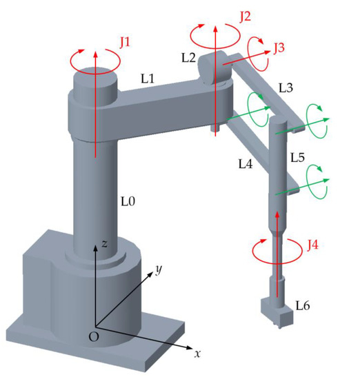
Figure 1.
The RRFbR robot (red: actuated revolute joints; green: passive revolute joints).
The seven links of the RRFbR manipulator, L0…L6, are connected by seven revolute joints. According to the Chebychev–Grübler–Kutzbach criterion [1], six moving rigid bodies (L1…L6) and seven revolute joints correspond to 1-DOF mobility (6 × 6 − 7 × 5 = 1), but the planar four-bar mechanism has three redundant constraints since its joint axes are parallel. By eliminating these redundant constraints, the 4-DOF mobility is obtained. The four actuated revolute joints (J1…J4) are represented in red in Figure 1. The corresponding rotation angles, shown in the kinematic scheme of Figure 2, represent the internal coordinates of the robot, collected in the vector θ = [θ1, θ2, θ3, θ4]T. The four external coordinates, composing the vector x = [x, y, z, θ]T, are the three Cartesian coordinates of the end-effector central point E with respect to the frame O(x,y,z) and the end-effector rotation θ about the z-axis of the same frame (Figure 2).
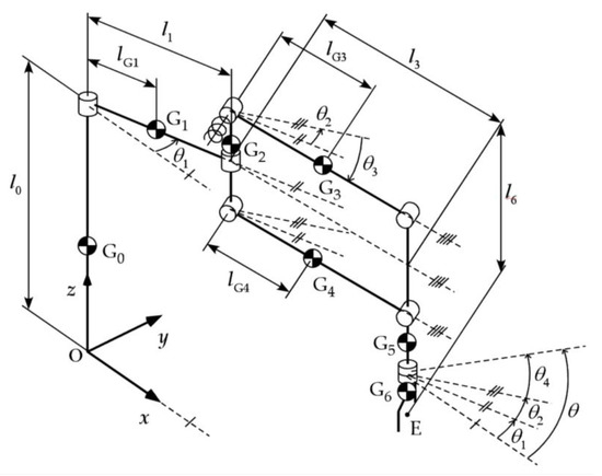
Figure 2.
Kinematic notation.
The kinematic and dynamic models of the manipulator are discussed in [11]. The dynamic model defines the relationship between the robot motion, the vector of the actuation torques τ = [τ1, τ2, τ3, τ4]T, and the vector of the generalized forces applied by the end-effector to the environment in the directions of the four external coordinates, F = [Fx, Fy, Fz, Mz]T [11].
Due to the robot architecture, gravity acts only on joint 3, since the rotations of joints 1, 2 and 4 do not influence the vertical position of the Center Of Mass (C.O.M.) of any link. Therefore, static balancing can be applied by adding a torsional spring acting on joint 3 in parallel with the actuator. The balancing spring, characterized by stiffness k3 and neutral position θ3p, can be mounted on any joint of the four-bar mechanism without changing its effect. As discussed in [17], even if the balancing spring should be tuned for any task to minimize energy consumption, a suitable compromise is to impose that the arm is exactly balanced when θ3 = 0 and in the absence of payload. This condition, which will be applied in this work, leads to a negative value of θ3p. The equations that define the spring parameters θ3p and k3 fulfilling this condition as a function of the robot’s geometrical and mass properties are discussed in [17].
3. Cartesian Space Position Control
Cartesian space position control of a generic serial manipulator is usually expressed by the following control law [18]:
In Equation (1): J(θ) is the robot Jacobian matrix; xd is the vector of the time-varying external coordinates of the set-point motion; τg(θ) is the gravity compensation; KKD is the stiffness matrix; DKD is the damping matrix. The superscript (i) designates the time derivative of fractional order i; therefore, in the law (1) damping is proportional to the derivative of order 1 of the error of the external coordinates.
In general, KKD and DKD define both the translational and the rotational behavior [18]; in the case of Schoenflies’ motion, their size is 4 × 4. In order to have the translational behavior decoupled from the rotational behavior, KKD and DKD are block-diagonal; the 3-DOF translational impedance is defined by the upper left 3 × 3 submatrices of KKD and DKD, while the 1-DOF rotational impedance is defined by the fourth diagonal elements of KKD and DKD.
The IO law (1) is named KD; a FO extension, named KDHD, is obtained by adding a damping term proportional to the derivative of order 1/2 (half-derivative) of the error through the 4 × 4 matrix HDKDHD [12]:
In (2) the half-derivative of f(t) is calculated through a digital filter with order n and sampling time Ts based on the Grünwald–Letnikov approach [19]:
The digital filter (3) considers only the time interval [t − nTs, t], while an exact calculation of a FO derivative involves all the time history of the original function. This introduces an approximation in the calculation of the FO derivative that modifies the stiffness imposed by the matrix KKDHD. To solve this problem, in Equation (2) a stiffness correction term is present, the function of HDKDHD and of the filter coefficients wj. The effectiveness of the control law (2) with the proposed correction is discussed in [12].
In the following, both the IO law (1) and the FO law (2) will be applied to the RRFbR manipulator, to assess if the type of Cartesian space position control influences the comparison of the motion profiles used to define the set-point motion xd. In the next section, the elliptic jerk motion profile’s main features will be summarized.
4. Elliptic Jerk Motion Profile
Figure 3 shows the elliptic jerk motion profile [10] in dimensionless formulation, adopted for the sake of generality. For any motion displacement d and motion duration T, it is possible to define:
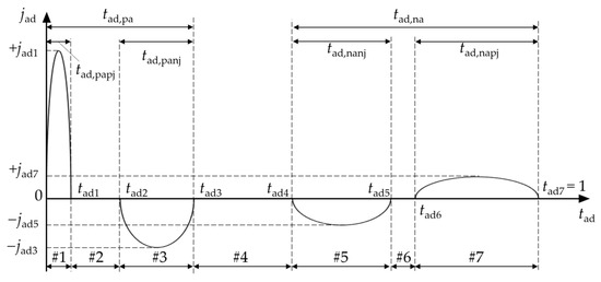
Figure 3.
Generic elliptic jerk profile.
- the dimensionless time, which is the time t divided by T: tad = t/T;
- the dimensionless position, which is the position s divided by d: sad = s/d;
- the dimensionless velocity, which is the velocity v divided by d/T: vad = vT/d;
- the dimensionless acceleration, which is the acceleration a divided by d/T2: aad = aT2/d;
- the dimensionless jerk, which is the jerk j divided by d/T3: jad = jT3/d.
The elliptic jerk profile is divided into seven phases (#1–#7, Figure 3). The i-th phase starts at tad,i−1 and ends at tad,i. Phases #1–#3 are characterized by positive acceleration, and their overall duration is tad,pa. The fourth phase is characterized by constant velocity and null acceleration. Phases #5–#7 are characterized by negative acceleration, and their overall duration is tad,na. Since the dimensionless duration of the motion is a unit, the duration of the fourth phase is (1 − tad,pa − tad,na).
Positive acceleration (phases #1–#3) is performed with a positive jerk in phase #1, with duration tad,papj, with a null jerk in phase #2, and with a negative jerk in phase #3, with duration tad,panj. Consequently, the duration of phase #2 is tad,pa − tad,papj − tad,panj (Figure 3). Similarly, deceleration (phases #5–#7) is performed with a negative jerk in phase #5, with duration tad,nanj, with a null jerk in phase #6, and with a positive jerk in phase #7, with duration tad,napj. Consequently, the duration of phase #6 is tad,na − tad,nanj − tad,napj (Figure 3).
For the phases with a non-null jerk (#1, #3, #5, and #7), the jerk profile is assumed to be elliptic. The jerk peaks of these phases are, respectively, +jad1, −jad3, −jad5, +jad7. Consequently, the dimensionless jerk profile is completely defined by ten positive parameters: four jerk peak parameters (jad1, jad3, jad5, jad7) and six time parameters (tad,pa, tad,na, tad,papj, tad,panj, tad,nanj, tad,napj). The acceleration, velocity and position profiles are obtainable by successive integrations, so they are defined by the same parameters.
Nevertheless, these parameters are not independent, since the following four conditions hold for a generic dimensionless rest-to-rest motion: null acceleration at the end of phase #3, null acceleration at the end of phase #7, the null velocity at the end of phase #7, and unit dimensionless displacement at the end of phase #7. These four conditions can be used to obtain the four jerk peak parameters as a function of the six time parameters. The analytical expressions of the dimensionless jerk, acceleration, velocity and position, and the expressions of the jerk peak parameters as functions of the time parameters are discussed in detail in [4] and are not reported here for reasons of space.
The number of independent dimensionless profile parameters can be further reduced by adding the following two hypotheses: tad,papj = tad,panj, and tad,nanj = tad,napj. It is possible to demonstrate that these two further assumptions lead to symmetric peak profiles both in acceleration and in deceleration (jad1 = jad3 and jad5 = jad7) [10]. It can be understood graphically considering that the integral of the jerk is the acceleration; consequently, if the semi-elliptical areas delimited by the jerk profiles of phases #1 and #3 are equal, the acceleration is null at the beginning of phase #4 (constant velocity); similarly, if the semi-elliptical areas delimited by the jerk profiles of phases #5 and #7 are equal, the acceleration is null at the end of the rest-to-rest motion. A profile fulfilling these conditions is named a symmetric elliptic jerk profile (Figure 4). For a symmetric elliptic jerk profile in dimensionless formulation, the number of independent parameters is four (tad,pa, tad,papj = tad,panj, tad,na, tad,nanj = tad,napj) [10].
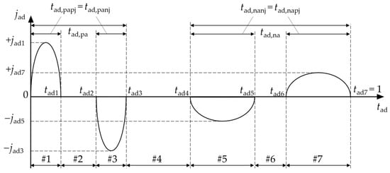
Figure 4.
Symmetric elliptic jerk profile.
In [10] the elliptic jerk motion profile (EJ) has been compared to other motion laws discussed in the scientific literature: the trapezoidal velocity profile (TV, [5]), the trapezoidal acceleration profile or S-curve (TA, [5]), the cycloidal profile (CY, [5]), the sinusoidal jerk profile (SJ, [20]), and the modified sinusoidal jerk profile (MSJ, [21]). Since the CY law cannot have finite phases with a null jerk, in order to include it in the comparison the durations of the phases of the EJ profile with a null jerk (#2, #4, #6) are imposed null. Moreover, the durations of the remaining phases (#1, #3, #5, #7) are imposed equally (1/4) [10]. With these assumptions, all the previously cited motion profiles are fully defined in dimensionless formulation, except the MSJ profile [10]. As a matter of fact, the MSJ profile is similar to the EJ profile, but each phase with a semi-elliptical jerk with a duration of 1/4 is replaced by a triplet of subphases: sinusoidal, constant, and sinusoidal [21]. In the comparison, these subphases have respective durations of 1/16, 1/8, and 1/16, with a total duration of 1/4. Overall, imposing all the discussed hypotheses, the comparison of the six motion profiles is shown in Figure 5 in terms of dimensionless jerk, acceleration, velocity and position.
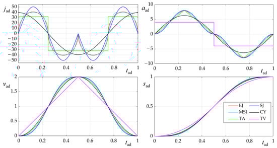
Figure 5.
Kinematic comparison of motion profiles in terms of dimensionless jerk jad, dimensionless acceleration aad, dimensionless velocity vad, and dimensionless position sad; elliptic jerk (EJ, red), sinusoidal jerk (SJ, blue), modified sinusoidal jerk (MSJ, cyan), cycloidal (CY, black), trapezoidal acceleration (TA, green), trapezoidal velocity (TV, magenta).
It is possible to note that the SJ profile has the highest jerk peak, 50.27, excluding the TV profile, which has infinite jerk, not represented. The EJ profile has a maximum jerk of 40.74, slightly higher than the CY, 39.48, and the MSJ, 39.11, while the TA profile has the lowest maximum jerk, 32.00. On the other hand, the jerk of the TA profile is discontinuous. Regarding the acceleration, the EJ, TA, SJ, and MSJ profiles have the same maximum, 8, while the CY and TV profiles have lower maxima, respectively, 2π and 4. With the considered hypotheses, all the profiles have the same maximum velocity, 2. In [10] the six profiles are compared with reference to a SISO second-order linear system. In the following, the same profiles will be applied to the rest-to-rest free motions of the RRFbR manipulator.
5. Multibody Model of the Manipulator
A multibody model of the RRFbR arm has been developed using Simscape MultibodyTM by MathWorks, neglecting friction in joints. The Cartesian space position control has been implemented using both the KD and the KDHD algorithms discussed in Section 3. Table 1 collects the geometrical and mass parameters of the manipulator.

Table 1.
Geometrical parameters and mass properties considered in the simulations.
Regarding the control parameters, for the KD controller: KKD is diagonal with kKD,x = kKD,y = kKD,z = 8 × 10³ N/m, and kKD,θ = 5 × 10² Nm/rad; DKD is diagonal with dKD,x = dKD,y = dKD,z = 5 × 10³ Ns/m, and dKD,θ = 7.5 Nms/rad.
For the KDHD controller, the stiffness matrix KKDHD is equal to KKD, all the values of the DKDHD matrix are halved with respect to DKD, and this diminution is compensated by the half-order damping, introduced by the HDKDHD matrix with hdKDHD,x = hdKDHD,y = hdKDHD,z = 22,500 Ns1/2/m, and hdKDHD,θ = 2.4 × 10⁴ Nms1/2/rad. These values have been obtained using the tuning criteria discussed in [17]. For the half-derivative digital filter of the KDHD controller, Ts = 0.005 s and n = 10; the same sampling time is used also for the KD controller.
6. Simulation Results
The set-point motion is composed of six phases. The start position xref corresponds to the robot arm semi-bent with internal coordinates θref = [−45°, 90°, 0°, −45°]T. In each phase: the end-effector moves in a time T from xref along a straight line with length d; it stops at xref + Δx for Tstop; it returns to xref along the same straight line; finally, it stops at xref for Tstop; then, the next phase begins. In the six phases, the displacements Δx are: (d, 0, 0); (0, d, 0); (0, 0, d); (−d, 0, 0); (0, −d, 0); (0, 0, −d); consequently, all the linear displacements are along one axis of O(x,y,z).
In each phase, there are two linear motions with opposite directions, characterized by the same duration T and displacement d. According to the definition of the dimensionless position and dimensionless time discussed in Section 4, these two parameters are used to scale in time and position the dimensionless profiles of Figure 5.
The end-effector rotation is maintained constant, since in robots with Schoenflies’ motion, the vertical rotation is dynamically decoupled from the translations, and in the following, the analysis is focused on the first three external coordinates.
Figure 6, Figure 7, Figure 8, Figure 9, Figure 10, Figure 11, Figure 12, Figure 13 and Figure 14 show the comparison of the motion profiles for the discussed six-phase motion with d = 0.15 m, T = 0.25 s, and Tstop = 3/5T = 0.15 s. In particular:
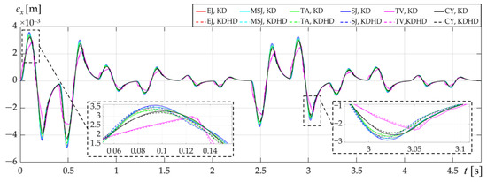
Figure 6.
Comparison of motion profiles: external coordinate error ex [m].
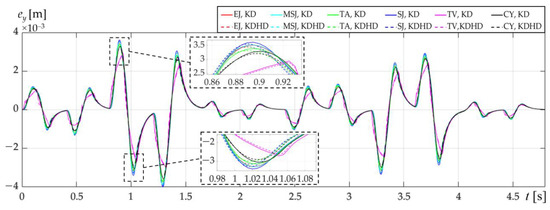
Figure 7.
Comparison of motion profiles: external coordinate error ey [m].
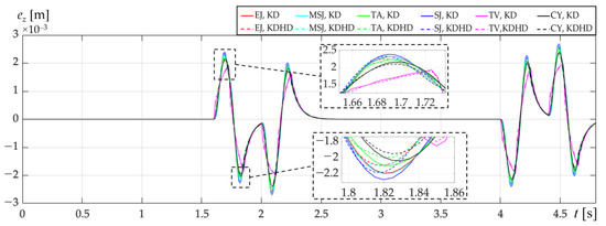
Figure 8.
Comparison of motion profiles: external coordinate error ez [m].
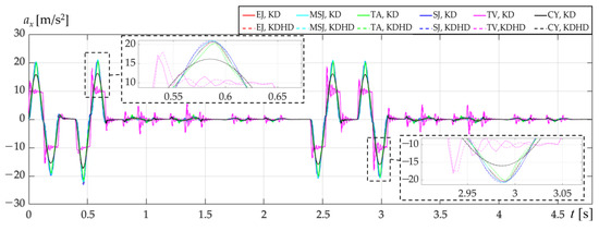
Figure 9.
Comparison of motion profiles: end-effector acceleration ax [m/s2].
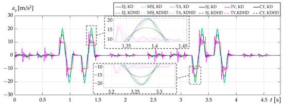
Figure 10.
Comparison of motion profiles: end-effector acceleration ay [m/s2].
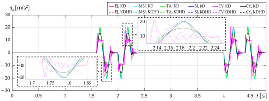
Figure 11.
Comparison of motion profiles: end-effector acceleration az [m/s2].
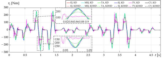
Figure 12.
Comparison of motion profiles: actuation torque τ1 [Nm].
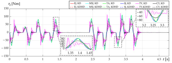
Figure 13.
Comparison of motion profiles: actuation torque τ2 [Nm].
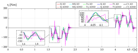
Figure 14.
Comparison of motion profiles: actuation torque τ3 [Nm].
The torque τ4 is not represented since it is null in the absence of friction and with constant end-effector orientation θ, as in the considered motion. The maximum absolute values of ex, ey, ez, ax, ay, az, τ1, τ2, and τ3 are collected in Table 2.
Table 2.
Maximum absolute values of external coordinates errors ex, ey, ez [mm], end-effector acceleration ax, ay, az [m/s2], and actuation torques τ1, τ2, τ3 [Nm].
In all the figures starting from Figure 6:
- continuous lines represent the results obtained with the KD controller, and dashed lines the results obtained with the KDHD controller;
- the colors of the graphs indicate the motion profile, with the same coding used in Figure 5.
From the analysis of Figure 6, Figure 7, Figure 8, Figure 9, Figure 10, Figure 11, Figure 12, Figure 13 and Figure 14 and of Table 2 it is possible to outline the following conclusions:
- once a motion profile is selected, the performance differences between the KD and KDHD controllers are not remarkable: as a matter of fact, all the graphs with continuous lines (KD) are qualitatively similar to the graphs with dashed lines (KDHD) of the corresponding color; as it will be discussed in the following, the benefits of the FO controller are higher for faster motions (see Figure 15, Figure 16, Figure 17 and Figure 18);
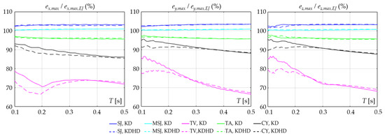 Figure 15. Maximum values of the x, y and z end-effector errors with different motion profiles (percentage ratios with respect to the elliptic jerk profile case).
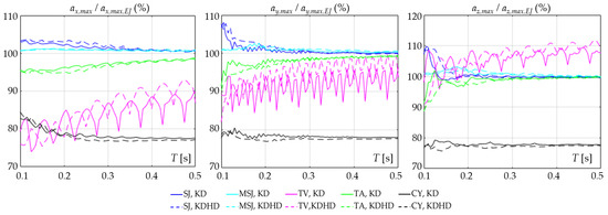 Figure 16. Maximum values of end-effector accelerations ax, ay, az with different motion profiles (percentage ratios with respect to the elliptic jerk profile case).
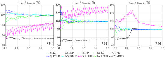 Figure 17. Maximum values of the actuation torques τ1, τ2, and τ3 with different motion profiles (percentage ratios with respect to the elliptic jerk profile case).
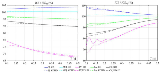 Figure 18. Integral Square Error and Integral Control Effort with different motion profiles (percentage ratios with respect to the elliptic jerk profile case).
 - as in SISO systems [10], the behaviors of the robot controlled by using the EJ, SJ and MSJ profiles are quite similar; nevertheless, observing the values of Table 2, it is possible to notice that the EJ profile performs slightly better, having lower maximum absolute values of the errors ex, ey, and ez than the SJ and MSJ profiles, but with similar values of the actuation torques τ1, τ2, τ3; also the acceleration values are slightly lower adopting the EJ profile rather than the SJ or the MSJ law;
- the TV, TA and CY laws allow to obtain lower errors; nevertheless, these profiles are characterized by jerk discontinuities [10], and this may cause vibrational phenomena which are not evidenced by the considered rigid body model; in particular, the TV profile has higher order discontinuities, since it has discontinuous acceleration and infinite jerk, while the TA and CY profiles have discontinuous but not infinite jerk; this causes oscillations of the actuation torques and of the end-effector accelerations with the TV profile (Figure 9, Figure 10, Figure 11, Figure 12, Figure 13 and Figure 14).
In order to investigate the effects of the motion speed, different simulations have been carried out with the same control parameters and with the same trajectory parameters of the results reported in Figure 9, Figure 10, Figure 11, Figure 12, Figure 13 and Figure 14 and in Table 2, but performing the motion at different speeds. This has been obtained by varying the motion duration T, which in the previous simulations was equal to 0.2 s, in the range between 0.1 s and 0.5 s, while maintaining the ratio Tstop/T = 3/5. Considering these assumptions, Figure 15, Figure 16 and Figure 17 represent the maximum absolute values of Table 2 (external coordinate errors, end-effector accelerations and actuation torques) as functions of the motion duration T. Moreover, Figure 18 shows, as overall indices of the error and of the actuation effort, the Integral Square Error of the end-effector translational coordinates (ISE) and the Integral Control Effort (ICE), defined according to the following expressions:
where Tsim is the simulation time, sufficient to evaluate adequately the residual vibrations.
In Figure 15, Figure 16, Figure 17 and Figure 18, all the performance parameters are expressed as percentage ratios of one parameter obtained with a specific motion law with respect to the same parameter obtained with the EJ profile. From the observation of these graphs, it is possible to outline the following conclusions:
- the benefits of the KDHD controller over the KD controller are greater for faster motions, with lower motion duration T, and using motion laws with higher discontinuities, in particular, TV and CY; for T = 0.1 s the percentage reduction in the maximum x, y and z end-effector errors using the FO controller are, respectively, −5.1%, −7.8% and −5.7% with the TV profile, and −0.9%, −3.4% and −5.8% with the CY profile (Figure 15);
- also considering the ISE, for T = 0.1 s the percentage reduction with the KDHD controller is −3.4% with the TV profile and −1.5% with the CY profile (Figure 18, left);
- this better accuracy is obtained even with a lower overall control effort: for T = 0.1 s the ICE reduction with the KDHD controller is −6.7% for the TV profile and −2.1% for the CY profile (Figure 18, right);
- on the other hand, if T increases (slower motions) the advantage of the KDHD controller over the KD in terms of ICE decreases gradually (Figure 18, right); for T = 0.5 s the ICE is almost equal and the differences in terms of maximum absolute and integral square errors are below 1%, with a slight advantage for the IO controller;
- focusing on the comparison among the motion profiles, it is possible to see that, with the considered rigid body modeling, the profiles with higher discontinuities (TV, TA, CY) have in general lower error, both in terms of maximum absolute values (Figure 15) and of ISE (Figure 18, left), independently of the motion speed, but also higher torque peaks for τ2, up to +18%, and for τ3, up to +47% (Figure 17);
- limiting the comparison to the smoother profiles (EJ, SJ, MSJ), more suitable for real systems, the EJ profile performs better than the other two, in particular with respect to the SJ: the increase in maximum absolute error with the SJ profile with respect to the EJ is up to +3.3% for all the three coordinates (Figure 15), while the increase in ISE is +3.8% (Figure 18, left); the error increase with the MSJ profile with respect to the EJ is lower, up to +0.8% for the maximum absolute errors and up to +0.7% for the ISE;
- it is interesting that the EJ profile allows obtaining lower error with lower control effort: the maximum ICE increase with respect to EJ is +8.2% with the SJ law for T = 0.1, and +1.3% with the MSJ law, for T = 0.16 (Figure 18, right); as regards the maximum values of the actuation torques (Figure 17), they are higher for the SJ and MSJ profiles with respect to the EJ in almost all the range of motion duration T.
7. Conclusions
In this paper, the application of the elliptic jerk profile (EJ) to position control of an RRFbR robot has been studied, comparing it to other motion profiles: sinusoidal jerk (SJ), modified sinusoidal jerk (MSJ), cycloidal (CY), trapezoidal acceleration (TA), and trapezoidal velocity (TV). Regarding the controller, both a classical IO algorithm (KD) and a FO alternative (KDHD) have been considered in order to evaluate how the type of controller influences the motion profile comparison.
Simulation results have shown that the influence of the controller type is lower than the influence of the motion profile, even if the KDHD controller is more efficient for fast motions, allowing to obtain lower maximum and integral errors even if the control effort is lower, especially in combination with the TV and CY profiles. On the contrary, for slower motions, the KD controller is slightly more accurate, with similar control effort, independently of the motion profile.
With the considered rigid body model, the TV, TA and CY profiles, with acceleration discontinuities (TV) and jerk discontinuities (TA and CY) offer better performance (lower maximum and integral errors in correspondence with lower control effort). Nevertheless, it is well known that proper limitations on jerk discontinuities should be respected for limiting vibrational phenomena in real systems with distributed elasticity, adopting smoother motion profiles [5].
The proposed EJ profile has continuous jerk, as the SJ and MSJ laws. The behavior of the considered robotic system with these three profiles is quite similar, as it occurs for the second-order SISO linear system discussed in [10]. As a matter of fact, this is due to the similar concept of these profiles, which starts from an alternation of phases with null jerk and phases with symmetrical jerk shape. For the SJ profile, the jerk shape is sinusoidal, for the MSJ the shape is sinusoidal modified with a constant section (constant maximum jerk for a finite time), and for the EJ profile the shape is elliptic. Even if the conception of these motion laws is similar, it is interesting to notice that the EJ profile shows a moderate advantage over the SJ and MSJ laws both in terms of accuracy (lower maximum absolute values of the end-effector errors, Figure 15, and of the ISE, Figure 18, left) and in terms of control effort (lower ICE, Figure 18, right).
8. Future Work
In future work, some planned research directions dealing with the proposed motion profile are the following:
- the comparison of the EJ profile to other motion laws with reference to second-order SISO linear systems, already discussed in the time domain in [10], will be carried out also in the frequency domain to obtain more general results;
- then the comparison will be extended to mechatronic axes with gearboxes, which are SISO systems characterized by strong nonlinearities (static friction, backlash), both in the case of ordinary gearheads [22] and of epicyclical gearboxes [23,24];
- the multibody simulation results on the RRFbR manipulator will be experimentally validated realizing a prototype of the manipulator; the scope of this prototype is not only related to motion planning but also to promote its usefulness in replacing the widespread SCARA architecture in the industry with energy-saving purposes, thanks to its static balancing;
- remaining in the fields of robotics, the EJ profile will be compared to other motion laws for position control of flexible mechanisms, more subject to the problem of relevant residual vibrations [25]; in particular, the prototype of a Cartesian parallel robot with elastic joints realized by superelastic inserts [26] will be exploited.
Author Contributions
Conceptualization, L.B. and D.S.; methodology, L.B.; software, L.B.; validation, L.B. and D.S.; formal analysis, L.B.; investigation, L.B.; resources, L.B.; data curation, L.B.; writing—original draft preparation, L.B.; writing—review and editing, L.B. and D.S. All authors have read and agreed to the published version of the manuscript.
Funding
This research received no external funding.
Institutional Review Board Statement
Not applicable.
Informed Consent Statement
Not applicable.
Data Availability Statement
Data is contained within the article. The simulation data presented in this study are available in figures and tables.
Conflicts of Interest
The authors declare no conflict of interest.
References
- Mallik, A.K. Kinematic Analysis and Synthesis of Mechanisms; CRC Press: London, UK, 2021. [Google Scholar]
- Wang, Y.; Belzile, B.; Angeles, J.; Li, Q. Kinematic analysis and optimum design of a novel 2PUR-2RPU parallel robot. Mech. Mach. Theory 2019, 139, 407–423. [Google Scholar] [CrossRef]
- Beyaz, A.; Dagtekin, M. Kinematic Analysis of Tractor Engine Crank-Rod Mechanism. Çukurova Univ. J. Fac. Eng. Archit. 2018, 33, 93–100. [Google Scholar]
- Wit, C.C.; Siciliano, B.; Bastin, G. Theory of Robot Control; Springer: London, UK, 2012. [Google Scholar]
- Biagiotti, L.; Melchiorri, C. Trajectory Planning for Automatic Machines and Robots; Springer: Berlin/Heidelberg, Germany, 2008. [Google Scholar]
- Constantinescu, D.; Croft, E.A. Smooth and time-optimal trajectory planning for industrial manipulators along specified paths. J. Robot. Syst. 2000, 17, 233–249. [Google Scholar] [CrossRef]
- Kyriakopoulos, K.J.; Saridis, G.N. Minimum jerk path generation. In Proceedings of IEEE International Conference on Robotics and Automation (ICRA), Philadelphia, PA, USA, 24–29 April 1988; pp. 364–369. [Google Scholar]
- Scalera, L.; Giusti, A.; Vidoni, R.; Gasparetto, A. Enhancing fluency and productivity in human-robot collaboration through online scaling of dynamic safety zones. Int. J. Adv. Manuf. Technol. 2022, 121, 6783–6798. [Google Scholar] [CrossRef]
- Stretti, D.; Bruzzone, L. Motion profiles with elliptic jerk. Mech. Mach. Sci. 2022, 122, 45–53. [Google Scholar] [CrossRef]
- Stretti, D.; Fanghella, P.; Berselli, G.; Bruzzone, L. Analytical expression of motion profiles with elliptic jerk. Robotica 2023, 1–15. [Google Scholar] [CrossRef]
- Bruzzone, L.; Bozzini, G. A statically balanced SCARA-like industrial manipulator with high energetic efficiency. Meccanica 2011, 46, 771–784. [Google Scholar] [CrossRef]
- Bruzzone, L.; Polloni, A. Fractional Order KDHD impedance control of the Stewart Platform. Machines 2022, 10, 604. [Google Scholar] [CrossRef]
- Bruzzone, L.; Fanghella, P. Comparison of PDD1/2 and PDμ position controls of a second order linear system. In Proceedings of the IASTED International Conference on Modelling, Identification and Control, MIC 2014, Innsbruck, Austria, 17–19 February 2014; pp. 182–188. [Google Scholar] [CrossRef]
- Bruzzone, L.; Fanghella, P. Fractional-order control of a micrometric linear axis. J. Control Sci. Eng. 2013, 2013, 947428. [Google Scholar] [CrossRef]
- Makino, H.; Furuya, N. Selective compliance assembly robot arm. In Proceedings of the First International Conference on Assembly Automation, Brighton, UK, 25–27 March 1980; pp. 77–86. [Google Scholar]
- Hervé, J.M. The Lie group of rigid body displacements, a fundamental tool for mechanism design. Mech. Mach. Theory 1999, 34, 719–730. [Google Scholar] [CrossRef]
- Bruzzone, L.; Nodehi, S.E. Application of Half-Derivative Damping to Cartesian Space Position Control of a SCARA-like Manipulator. Robotics 2022, 11, 152. [Google Scholar] [CrossRef]
- Bruzzone, L.; Molfino, R.M. A geometric definition of rotational stiffness and damping applied to impedance control of parallel robots. Int. J. Robot. Autom. 2006, 21, 197–205. [Google Scholar] [CrossRef]
- Das, S. Functional Fractional Calculus; Springer: Berlin/Heidelberg, Germany, 2011. [Google Scholar]
- Valente, A.; Baraldo, S.; Carpanzano, E. Smooth trajectory generation for industrial robots performing high precision assembly processes. CIRP Ann. Manuf. Technol. 2017, 66, 17–20. [Google Scholar] [CrossRef]
- Fang, Y.; Qi, J.; Hu, J. An approach for jerk-continuous trajectory generation of robotic manipulators with kinematical constraints. Mech. Mach. Theory 2020, 153, 103957. [Google Scholar] [CrossRef]
- Concli, F.; Gorla, C.; Stahl, K.; Hoehn, B.-R.; Stemplinger, J.-P.; Schultheiss, H. Load independent power losses of ordinary gears: Numerical and experimental analysis. In Proceedings of the 5th World Tribology Congress, WTC 2013, Turin, Italy, 8–13 September 2013; Volume 2, pp. 1243–1246. [Google Scholar]
- Bilancia, P.; Monari, L.; Raffaeli, R.; Peruzzini, M.; Pellicciari, M. Accurate transmission performance evaluation of servo-mechanisms for robots. Robot. Comput. Integr. Manuf. 2022, 78, 102400. [Google Scholar] [CrossRef]
- Fanghella, P.; Bruzzone, L.; Ellero, S.; Landò, R. Kinematics, efficiency and dynamic balancing of a planetary gear train based on nutating bevel gears. Mech. Based Des. Struct. Mach. 2016, 44, 72–85. [Google Scholar] [CrossRef]
- Boscariol, P.; Scalera, L.; Gasparetto, A. Nonlinear control of multibody flexible mechanisms: A model-free approach. Appl. Sci. 2021, 11, 1082. [Google Scholar] [CrossRef]
- Bruzzone, L.; Molfino, R.M. A novel parallel robot for current microassembly applications. Assem. Autom. 2006, 26, 299–306. [Google Scholar] [CrossRef]


Disclaimer/Publisher’s Note: The statements, opinions and data contained in all publications are solely those of the individual author(s) and contributor(s) and not of MDPI and/or the editor(s). MDPI and/or the editor(s) disclaim responsibility for any injury to people or property resulting from any ideas, methods, instructions or products referred to in the content. |
© 2023 by the authors. Licensee MDPI, Basel, Switzerland. This article is an open access article distributed under the terms and conditions of the Creative Commons Attribution (CC BY) license (https://creativecommons.org/licenses/by/4.0/).