Abstract
An efficient and accurate method for concrete thermal parameter inversion is essential to guarantee the reliable and prompt thermal analysis results of dams. Traditional inversion methods either suffer from low analysis efficiency or are limited in accuracy. Thus, this paper presents a method for multiple thermal parameter inversion based on an integrated surrogate model (ISM) and the Jaya algorithm. This method replaces finite element analysis with an ISM incorporating three machine learning algorithms, Kriging, support vector regression (SVR), and radial basis function (RBF), to describe the mapping relationship between thermal parameters and structure temperature responses. The input datasets for model training and testing are generated by a uniform design approach. Subsequently, a simple and efficient global optimization algorithm, Jaya, is used to identify the thermal parameters by minimizing the error between calculated and monitored temperatures. The effectiveness and practicality of this method are verified by applying monitored data of two strength grades of concrete in a dam. The verification results indicate that the proposed approach can obtain more accurate inversion results than the above individual models. Compared with these models, the inversion errors using ISM are reduced by 8.45%, 3.93% and 20.85%, respectively for C35 concrete, and by 6.53%, 23.82% and 44.43%, respectively for C40 concrete. Additionally, this approach maintains the powerful computational efficiency of surrogate-based optimization, and compared to the methods that directly invert using swarm intelligence algorithms, the analysis efficiency is improved by about 111.7 times.
1. Introduction
During the construction of concrete dams, thermal cracks on concrete may occur due to unfavorable temporal and spatial temperature variations, affecting the integrity and durability of its structure [1,2,3]. To avoid such cracks, the main idea is to use FEM to track the actual temperature load of the dam dynamically, and then design reasonable temperature control and crack prevention schemes based on the crack resistance of the concrete [4,5,6]. The thermal parameters represent the main thermal properties of concrete, which determine the performance of heat generation and transfer within the structure. Therefore, efficient and accurate access to thermal parameters is essential for obtaining reliable and prompt temperature analysis results. In the past, thermal parameters were primarily derived from laboratory tests, which required expensive equipment and long test cycles. Moreover, it is common that the thermal properties of concrete on-site differ significantly from the test results due to different production batches of raw material and different construction conditions [7]. In recent years, inversion analysis using concrete temperature monitoring data from construction sites has proven to be an effective method for obtaining parameters.
Parameter inversion analysis solves for the undetermined parameters of the model under specific initial and boundary conditions, so that the theoretical response calculated by the model approximates the observed response. In the early days, such calculations were often carried out with the simplex method [8], the conjugate gradient method [9] and the proposed Newton method [10]. However, these methods were not always appropriate for managing the inversion of concrete thermal parameters, for they are highly nonlinear, leading to unstable solutions during computation, which are prone to fall into local optimization regions or even non-convergence. With the development of cluster intelligence algorithms, algorithms with global search capabilities such as the genetic algorithm (GA) [11], differential evolution algorithm (DE) [12], particle swarm optimization algorithm (PSO) [13], and whale optimization algorithm (WOA) [14] were introduced into the concrete thermal parameters’ inversion. They alleviate the local optimum problem and improve the inversion accuracy. However, even though the intelligent optimization algorithm offers an easier path to the global optimal solution, more finite element calculations must be performed during each iteration to adjust the subsequent search direction. As a consequence, the computational cost is enormous, hindering the efficient analysis of dam temperature control schemes. Accordingly, a surrogate-based optimization (SBO) method [15] has emerged as a powerful analytical tool due to its ability to reduce computational costs while maintaining global search capability.
SBO’s core concept is to approximate the relationship between undetermined parameters and structural responses by performing a few expensive finite element analyses. In analyzing complex engineering problems, polynomial response surface (PRS), RBF, Kriging and SVR are the primary examples widely used to establish surrogate models. For example, Das [16] used PRS to establish a surrogate model that characterizes the relationship between a rockfill dam’s mechanical parameters and displacement response; Tullu [17] developed an RBF-based surrogate model for predicting inter-ply shear stresses during composite press forming; Wang [18] introduced the SBO method to the arch dam body design and developed a Kriging-based surrogate model for body shape parameters optimization; Chen [19] proposed a surrogate model based on SVR for identifying the thermophysical parameters of aircraft components. Meanwhile, applications of the SBO approach for thermal parameter inversion are also notable. Pei [20] proposed a PRS-based method for identifying concrete thermal parameters; Zhou [21] constructed a surrogate model using back propagation neural network (BPNN) and inverted the thermal parameters of a concrete dam; Wang [22] used SVR to reverse the thermal parameters based on the prototype monitoring temperature data and then compared the inversion accuracy with the BPNN. These approaches have increased the efficacy of inversion compared to the early days.
However, these methods have some limitations in terms of computational accuracy. Each surrogate model has distinct advantages facing different problem models, variables, and sample sets [23]. For instance, in the concrete thermal parameter inversion problem, there are many uncertainties, such as the inversion model’s extreme value characteristics, the range of thermal parameter values, the selection of the sample sets, etc. As a result, it is challenging to determine which model would best describe the complex nonlinear relationships between input and output variables. In recent years, the primary solution to such insufficient a priori information is to integrate several models by weighted combination. This method has been used in many fields, such as structural reliability analysis [24,25], mechanical performance optimization [26,27], groundwater simulation [28,29], etc. It has been demonstrated that this approach can incorporate the characteristics of multiple models and minimize the adverse effects caused by a single model, thus addressing the uncertainty in modeling and enhancing the overall fitting accuracy.
In this paper, the surrogate model integrating technology is introduced to the thermal analysis of concrete dams. An ISM combined with the Jaya optimization algorithm is proposed for multiple thermal parameters inverse analysis. The ISM consists of three linearly weighted sub-models: Kriging, SVR, and RBF. In comparison to a single model, the ISM combines the characteristics of several models, offering stronger robustness and a better description of the complex relationship between undetermined thermal parameters and structural temperature responses. To provide a more representative sample for the ISM, the input datasets for training and testing are generated by an efficient sampling method, uniform design. Based on the trained ISM, the Jaya algorithm minimizes errors between the calculated and monitored temperatures to obtain concrete thermal parameters. The Jaya algorithm is chosen because it has a simpler structure and no algorithmic parameters compared with other common global optimization algorithms such as PSO and GA. The method proposed in this paper helps to coordinate the accuracy and efficiency of the concrete thermal parameter inversion, which is of great importance for the structural safety of dams.
The structure of this paper is as follows: Section 2 introduces the inverse analysis methodology of ISM-Jaya for multiple thermal parameters; an engineering case study is employed in Section 3 to demonstrate the efficiency and accuracy of the proposed method, and conclusions and future work are drawn in Section 4.
2. Methodology
To accurately and efficiently invert thermal parameters, this paper proposes a multi-parameter inversion method using ISM. Figure 1 shows the flowchart of this method, which is divided into four parts: (1) the mathematical model construction for thermal parameter inversion, which transforms the parameter determination problem into an optimization problem; (2) sample set generation, which generates samples for the training and testing of the integrated surrogate model; (3) ISM construction, which is to determine the hyperparameters of the sub-models and the weight coefficients used for model integration; and (4) thermal parameter identification, which is the process of solving the aforementioned optimization problem. The principles and methods of each part are presented as follows.
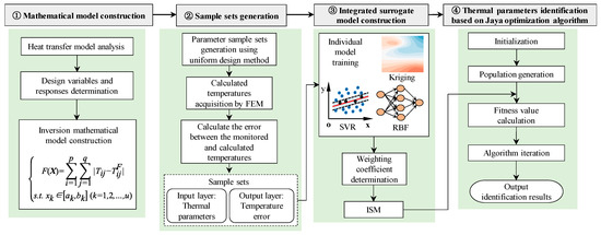
Figure 1.
Methodology flowchart of this study.
2.1. Mathematical Model Construction for Multiple Thermal Parameters Inversion
2.1.1. Calculation Theory of Temperature Field Containing Cooling Water Pipe
Heat transfer in a concrete dam is governed by the following [30]:
where is the concrete temperature; is the temperature conductivity; is the heat; is the specific heat of concrete; is the density of concrete; and is the time.
The temperature rise rate of concrete under adiabatic conditions is as follows:
where is the adiabatic temperature rise of the concrete.
The governing equation is subject to the following initial conditions:
where is the initial distribution function of temperature.
The boundary conditions of the external surface are as follows:
(1) First type:
(2) Second type:
(3) Third type:
where is the known temperature on the boundary; is the known heat flow on the boundary; is the direction of the external normal to the boundary; is the heat release coefficient; and is the air temperature.
Many serpentine cooling pipes are arranged in the concrete dams to regulate the concrete temperature, as shown in Figure 2a. In a concrete cylinder of diameter length , as shown in Figure 2b, the inlet water temperature of the water pipe is , and the final adiabatic temperature rise is . Assuming that the outer surface of the cylinder is adiabatic, the average temperature of the concrete can be expressed as follows:
where and are the outer and inner radius of the concrete column, respectively; is the inner radius of the cooling water pipe; and are the thermal conductivity of concrete and cooling water pipe, respectively; is the specific heat of cooling water; is the density of cooling water; is the flow rate of cooling water; and are the horizontal and vertical spacing of the cooling water pipe, respectively; is a function related to the adiabatic temperature rise in the concrete.
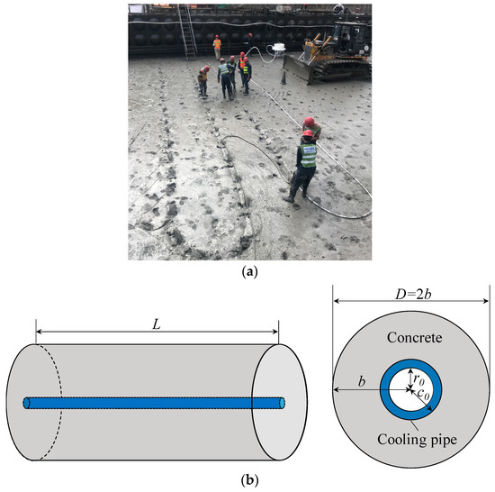
Figure 2.
Diagram of the water pipe cooling for concrete. (a) describes the laying of cooling water pipes; (b) describes the simplified treatment of water pipe cooling.
Before constructing a mathematical model for the adiabatic temperature rise in the concrete, a functional expression is usually assumed and then fitted with experimental data. Commonly available forms are exponential, hyperbolic, double exponential, and combined exponential. The combined exponential model matches the test data better and is widely used in engineering [30]. The expressions are as follows:
where , , and are the coefficients to be determined, .
can be expressed as
2.1.2. Mathematical Model Construction
According to Section 2.1.1, in the concrete temperature field analysis, the primary thermal parameters of concrete are temperature conductivity , thermal conductivity , adiabatic temperature rise , specific heat , density , and heat release coefficient . Concrete density and specific heat can be obtained accurate and stable values by testing. Moreover, there is a definite relationship:
Therefore, the thermal parameters to be inverted are the temperature conductivity (or thermal conductivity), the adiabatic temperature rise, and the surface heat release coefficient.
FEM-based thermal parameter inversion of concrete can be regarded as an optimization problem. With the optimization criterion of minimizing the error between the monitored and calculated temperatures, the concrete thermal parameters are identified by an optimization algorithm. Assuming that the dam concrete is an isotropic homogeneous material, the mathematical model for the inversion analysis can be expressed as
where is the objective function; is the parameter vector to be inverted; and is the number of parameters to be inverted. and are the numbers of temperature measurement point and monitoring sequence, respectively; and are the total number of measurement points and the monitoring times, respectively; and are the monitoring temperature and calculation temperature, respectively; are the feasible domains of the parameters to be inverted.
2.2. Experimental Design and ISM Construction
Section 2.1 determines the design variables and structural response of the thermal parameter inversion problem. An approximate model can be adopted to describe the relationship between the two according to Equation (11), thus replacing the finite element analysis in the optimization iteration. This study uses the surrogate model integration technique to develop the approximate model.
ISM consists of a linear overlay of multiple individual surrogate models in the hope of counteracting errors in prediction through appropriate weighting. In this paper, among the commonly used surrogate models, Kriging, SVR, and RBF, which have high prediction accuracy in dealing with nonlinear problems [23,31,32], are selected to construct the ISM. The prediction result can be expressed as
where is the weight coefficient, is the individual surrogate model, and is the number of surrogate models.
The key to constructing an ISM is the weight coefficient determination. In general, the weights of the surrogate model should reflect our confidence in the model and filter out adverse effects. The current approach to determining the weight coefficients is mainly based on the generalized mean square error (). Assuming there are training samples, a surrogate model is constructed times, each time leaving out one of the training samples. Subsequently, the global error is evaluated using the difference between the exact response at the omitted sample and the predicted value:
where is the exact response at , and is the corresponding predicted response from the surrogate model constructed using all except ().
In this point, a surrogate model with a small will have a large weight in the ISM. The Ref [33] provides a heuristic method for obtaining weights with the following equation:
where is the of the th surrogate model. and , two parameters that require the user to specify, describe the importance of and , respectively, and . Small values of and large negative values of assign high weights to the best surrogate model. In contrast, large values of and small negative values of assign relatively balanced weights to individual surrogate models. The recommended values are = 0.05, = −1.
The experimental points used for model training and testing should be sufficiently representative to ensure the satisfactory generalization performance of the ISM. In contrast, if not properly constructed, the reliability of both the integrated and individual surrogate models can hardly be guaranteed. As a result, it is essential to design appropriate datasets for model training and testing.
The uniform design method is used in this research to generate training and test samples for ISM. Uniform design [34,35] is one of the most widely used sampling methods, which can effectively capture the critical information in the design space without sufficient a priori information. It also has the advantages of simple operation and efficient sampling and is widely used in complex systems modeling.
In addition, the performance of the constructed model is evaluated by the determination coefficient [36,37].
2.3. Jaya Algorithm
The Jaya algorithm [38] is a simple but efficient optimization algorithm built on the core concept of constantly approaching the optimal solution and moving away from the worst solution. It only requires setting conventional algorithm parameters such as population size and iteration number, and no other parameters, reducing the algorithm testing workload and the chance of falling into local optimum. As a consequence, compared to other population-based heuristics, the Jaya algorithm outperforms them regarding search accuracy and convergence performance [39,40]. This algorithm’s revised formula is as follows:
where is the current candidate solution, is the number of iterations, is the population size, is the number of design variables; and are the best and worst solution among the candidate solutions, respectively; and are two random values from 0 to 1.
New candidate solutions can be generated continuously by Equation (15) until the iteration termination condition is reached.
2.4. ISM-Jaya for Multiple Thermal Parameters Inverse Analysis
This paper proposes a simple and efficient method based on the prototype monitoring temperature for multiple thermal parameter inversion of concrete dams.
The ISM replaces the complicated and time-consuming finite element analysis, at which point the thermal inverse analysis is transformed into a parametric optimization problem. The Jaya algorithm then minimizes the difference between the observed and calculated responses to identify the concrete thermal parameters.
The flowchart of the proposed ISM-Jaya method for multiple thermal parameter inversion of concrete dams is shown in Figure 3. The main steps are as follows.

Figure 3.
Flowchart of ISM-Jaya method for multiple thermal parameter inversion.
Step 1: Determine the thermal parameters of the concrete dam to be inverted, as well as the approximate range of these parameters, which can be referenced from experimental results or similar projects.
Step 2: Obtain the training and testing datasets for ISM. Design parameter sample sets using uniform design, which are input to the finite element model for temperature analysis one by one. The error between the monitored and calculated temperatures is calculated using Equation (11). Thus, the training and test sets consisting of the parameter samples and temperature errors are obtained.
Step 3: Construct the ISM. Based on the sample set obtained in Step 2, the ISM could be trained and tested with the thermal parameters as inputs and the temperature errors as outputs, until it meets the accuracy requirements for replacing the finite element analysis. Otherwise, it is necessary to return to Step 2 and increase the sample size.
Step 4: Parameter inversion. Several sets of initial parameters are generated as the initial population within the range of thermal parameters, and the fitness value of each individual is calculated by the trained ISM in step 3 to obtain the candidate solution set. Based on the optimal and worst solutions in the current candidate solution set, the positions of the individuals in the next iteration are updated with the optimization objective of minimizing the error between the monitored and calculated temperatures.
Step 5: Inversion result output. The inversion results are obtained when the Jaya algorithm termination condition is reached.
3. Case Study
3.1. Project Background
The concrete hyperbolic arch dam in southwest China has a maximum height of 285.5 m. As shown in Figure 4, the dam’s concrete is divided into three zones, A, B, and C, which correlate to three strength grades of C40, C35, and C30, respectively. Because various grades of concrete have different thermal properties, it is essential to identify the thermal parameters of concrete in distinct partitions, and Zone A and Zone B are chosen for inversion in this study.
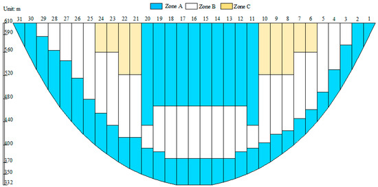
Figure 4.
Zoning diagram of dam concrete.
To acquire concrete temperature data, we deployed distributed fiber optic temperature sensing systems in four dam sections (5#, 15#, 16#, and 23#). The fiber optic arrangement scheme of typical pouring blocks is shown in Figure 5a. The fiber optic is located in the middle of two layers of cooling water pipes and is used to monitor the internal temperature of the pouring block, as shown in Figure 5b,c. This section uses bifilar fiber optics to facilitate the spatial positioning of temperature measuring points along the cable [41]. The temperature measurement system’s temperature resolution is 0.01 °C, the measurement accuracy is 0.1 °C, and the spatial resolution is 1 m. The distribution of temperature measurement points is schematically shown in Figure 5d.
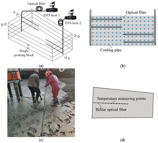
Figure 5.
Distributed fiber arrangement diagram. (a) describes the overall optical fiber arrangement scheme; (b,d) describe the A-A and B-B profiles in (a), respectively; (c) describes the construction technics for embedding bifilar optical fiber.
3.2. Finite Element Model and Boundary Conditions
According to the construction information provided by the contractor, the 15# dam section under construction was selected to establish a three-dimensional finite element model. The coordinates were the X-axis in the transverse direction, Y-axis in the downstream direction, and Z-axis in the vertical direction. The mesh is divided by 8-node hexahedral elements, with 21,664 elements and 26,505 nodes, as shown in Figure 6. The range of mesh size along X, Y and Z directions are 2.75~3.00 m, 3.58~6.11 m and 0.33~0.75 m, respectively. The construction process of the pouring block was simulated using the birth and death element technique, which first kills all the elements, and then activates each pouring block according to the construction progress.
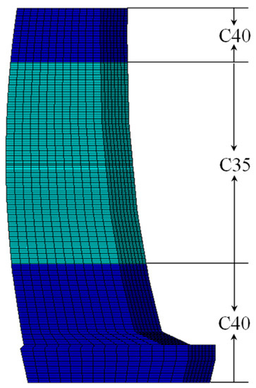
Figure 6.
Finite element mesh model.
The surface temperature of the dam is affected by various factors such as air temperature, solar radiation, wind, and curing measures, so the equivalent surface heat release coefficient [42] is used to reflect the heat exchange performance of concrete and air. Before being covered by concrete, the sides are supposed to be a third-type boundary condition, and an adiabatic boundary after being covered. The upstream, downstream, and top surfaces are considered third-type boundary conditions.
The initial temperature of the concrete was assumed to be the placing temperature. The water cooling was applied immediately after the completion of concrete pouring, and the water inlet and outlet were reversed every 24 h. Air temperature and water pipe cooling parameters such as water temperature and flow rate were obtained according to the monitoring records. The ground temperature at the bottom of the dam is a constant 20 °C.
The temperature coefficient , the adiabatic temperature rise model parameters , , and , as well as the equivalent heat release coefficient , are the thermal parameters that need to be inverted according to the analysis in Section 2. In addition to the above, the parameters of the cooling pipe are shown in Table 1, and the other material parameters are shown in Table 2.

Table 1.
Parameters of the cooling water pipe.
Table 2.
Parameters of the other material.
3.3. Predictive Performance Analysis of Different Surrogate Models
In each material division, three pouring blocks (C35: 15#-52~15#-54, C40: 15#-57~15#-59) were chosen according to the fiber arrangement.
Three pouring blocks (C35: 15#-52~15#-54, C40: 15#-57~15#-59) were selected in each material partition according to the fiber arrangement. The average value of all measured points within a single casting block was taken as its mean temperature and used for inversion analysis to mitigate the effect of uneven local temperature distribution.
The value range of thermal parameters of dam concrete is determined [30], as shown in Table 3. Surrogate model training and testing samples were generated by uniform design, and the sample sizes include 10, 20, 40, 60, 80, 100, and 120, in which 10 was used as the test sample and the rest were training samples. The parameter combinations in each sample set were input to the finite element model one by one to calculate the temperature field, obtaining the calculated temperature at the center point of the above pouring blocks. Based on the calculated temperature and the aforementioned monitored temperature, the error between the two was estimated by Equation (11), completing the generation of different sample sets.
Table 3.
The range of parameters.
On this basis, integrated and individual surrogate models are built separately to compare their predictive performance. Since the correlation function of the Kriging model, the kernel function of the SVR model, and the activation function of the RBF model play significant roles in their respective predictive performance, studies have proven that using the Gaussian model can lead to superior results in solving nonlinear problems [43,44,45]. Thus, in this study, the Gaussian model has been selected. The hyperparameters of the models significantly affect the generalization performance. The determination methods were as follows [24,31]. The hyperparameters of the Kriging model were determined using maximum likelihood estimation. The SVR model’s penalty factor and width parameters were determined using the Jaya algorithm with a population size of 20 and a maximum number of iterations of 100. The width parameters of the RBF model were determined using the Jaya algorithm with a population size of 10 and a maximum number of iterations of 20.
The R2 of the test results for different training samples is shown in Figure 7.
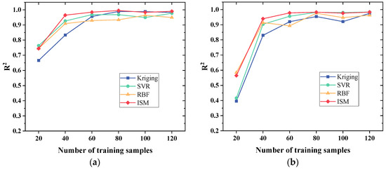
Figure 7.
Comparison of test results based on different sample sets. (a,b) describe the comparison results for C35 and C40 concrete, respectively.
As shown in Figure 7, as the sample size increases, the overall prediction accuracy of each surrogate model first exhibits an increase and then reaches stabilization. The reason for this is the density of sample points increases, adding critical information to the whole design space, which has a boosting effect on the predictive performance. When the sample size reaches a certain level, increasing the sample again does not improve predictive performance much, and may even show a sign of decreasing. This indicates that the model already has satisfactory predictive performance for an ideal sample size with sufficient critical information. In addition, there is a risk of overfitting in the model due to monitoring noise, which causes degraded prediction performance. Theoretically, this can be solved by continuously increasing the sample size, but this implies higher FEM computational costs, contrary to the original intention of improving the efficiency for parameter inversion.
In this study, the parameters to be inverted for the two types of concrete are the same, but the differences in thermal properties and construction conditions will cause differences in the inversion problem model. Therefore, the predictive performance of the individual models can be compared from two aspects: problem model and sample size.
In the same problem model, as shown in Figure 7a, when the sample size is 60 or less, the predictive accuracy of the SVR model reaches its peak. While the sample size is larger than 60, the Kriging model has the highest accuracy. In Figure 7b, when the sample size is 40 or less, the Kriging model has the highest predictive accuracy; while the sample size is larger than 40, the SVR model performs the best. With the same sample size, it is equally difficult to determine which model to use when dealing with different problem models. For example, when the sample sizes are 80 and 100, the Kriging model has the highest accuracy in C35 concrete, while the opposite is true in C40 concrete. This indicates that for different inversion problem models and sample sizes, the prediction accuracy of the three individual surrogate models behaves differently, with no one consistently outperforming the other. This reflects the uncertainty of the thermal parameter inversion problem. In other words, it is risky to directly choose a particular surrogate model to replace the finite element analysis.
Combined with the previous analysis, these models can perform well with an ideal size of samples. However, this is relative to some defined problem models and a defined range of variables. In reality, it is problematic that their relationship lacks a priori information, so the focus should be on ensuring the robustness of the surrogate model to weaken this effect.
Figure 7 shows that for different problem models and sample sizes, the predictive accuracy is always better than or close to that of the individual model with the best prediction. Moreover, the accuracy index of the ISM has the same trend as that of the individual surrogate model, indicating that its predictive performance relies on the individual model. The ISM does not have an overwhelming improvement in predictive accuracy relative to individual ones; its most significant advantage lies in mitigating the influence caused by the aforementioned lack of prior information and improving the robustness of the model. In addition, the ISM requires a smaller sample size to achieve stable accuracy, which is an advantage for a more efficient inversion of concrete thermal parameters.
3.4. Analysis and Discussion of Inversion Results
The predictive performance on the test samples is only a part of the thermal parameter inverse analysis based on the surrogate model. Regardless of choices, the test set is only a tiny part of the sample space after all. So, the inversion results are compared in this section.
3.4.1. Inversion Results Based on the ISM
It can be seen in Figure 6 that the R2 variation of the integrated agent model is slight when the sample size is greater than 60. Thus, the ISM with a training sample size of 60 is selected to replace the finite element model. The Jaya algorithm invokes the trained integrated agent model for inversion with a population size of 40 and a maximum iteration number of 200. The inversion results are shown in Table 4.
Table 4.
Inversion results.
Since the actual thermal parameter values are unknown on the construction sites, the reliability of its results cannot be directly verified. The common approach to this problem is to use FEM to obtain the calculated temperature based on the inversion results and evaluate the degree of agreement between this temperature and the monitored one.
According to the assumptions mentioned earlier, the adiabatic temperature rise model ignores the influence of factors other than age on the hydration process, the homogenization treatment of concrete materials, etc. These factors are difficult to describe accurately in the temperature analysis of dams under construction, but will undoubtedly cause deviations between the calculated and monitored temperatures. To prevent overfitting, the global agreement of the temperature should be used to evaluate the reliability of the inversion results. The mean absolute error (MAE) is quantified in this article, and Figure 8 depicts a comparison of the calculated and monitored temperatures.
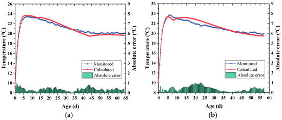
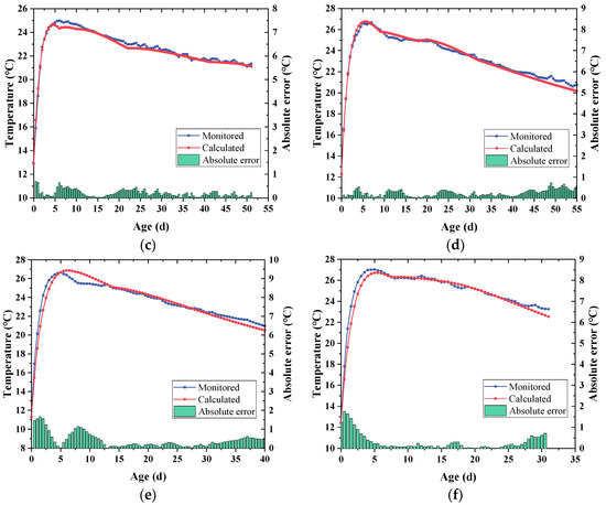
Figure 8.
The comparison of calculated and monitored temperatures. (a–c) describe the temperature comparison results of 15#-52–15#-54 pouring blocks, respectively; (d–f) describe the temperature comparison results of 15#-57–15#-59 pouring blocks, respectively.
From Table 4, it may be noted that the inversion results vary for the two concretes; therefore, it is necessary to invert the parameters by sub-regions for concrete.
According to Figure 8, in the beginning, the heat dissipation rate of the pouring block surface and water pipe cooling is lower than the heat release rate of cement hydration, resulting in the accumulation of heat inside the cast block and causing the temperature to rise until it reaches the maximum value rapidly. As the heat release rate decays, the surface heat dissipation and water pipe cooling begin to dominate, leading to a gradual decrease in concrete temperature. It can be found that the overall variation of the calculated and monitored temperatures tends to be consistent, with stage deviations mainly concentrate in the early times, especially in the temperature rise phase, as shown in Figure 8e,f. The main reasons for these deviations between the two are related to the aforementioned calculation assumptions. The MAE of the C35 and C40 concrete pouring blocks were 0.32 °C and 0.31 °C, respectively, with maximum errors of 1.02 °C (15#-53) and 1.75 °C (15#-59).
The agreement between their monitored and calculated temperatures was supervised in the inverse analysis for the above six pouring blocks, while the other pouring blocks were not. To further investigate the universality of the inversion results, one pouring block was selected from zone A and another from zone B, neither participating in the sample set generation. The degree of agreement between the calculated and monitoring results of each of these two blocks was then compared, as shown in Figure 9. The MAE of C35 and C40 were 0.59 °C and 0.73 °C, respectively. The maximum error of the C35 pouring block was 2.35 °C, which happened during the warming stage, after which the errors were within 1.5 °C. The maximum error of the C40 pouring block was 1.17 °C.
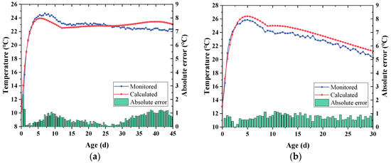
Figure 9.
The comparison of calculated and monitored temperatures. (a,b) describe the temperature comparison results of 15#-55 and 15#-60 pouring blocks, respectively.
Figure 10 shows the temperature field contours of the dam Section 15# at various construction stages based on the inversion results.
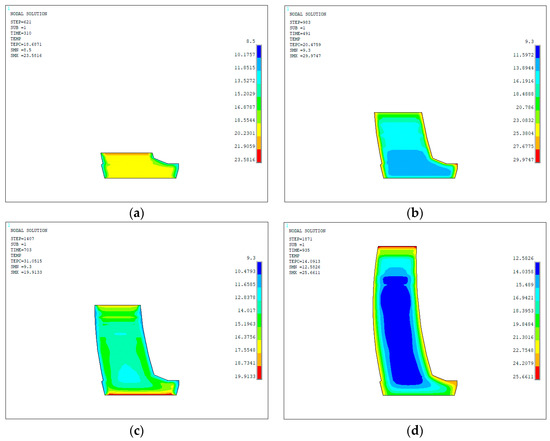
Figure 10.
Temperature distribution in different construction stages. (a–d) describe the temperature distribution of the 15# dam section up to EL.350m (in cold season), EL.395m (in hot season), EL.423.5m (in cold season) and EL.491m (in hot season) elevations, respectively.
Since this dam adopted staged water cooling to cool the concrete to the joint grouting temperature, as shown in Figure 10, the internal high-temperature zone migrated vertically during pouring during the construction period. Moreover, due to artificial cooling, the low-temperature zone expands in the same direction as the concrete cools to the grouting temperature. Furthermore, a uniform temperature distribution is observed within the dam except for a certain vertical temperature gradient in the upper part of each construction stage. The surface temperature of the dam is mainly influenced by the external ambient temperature, and the temperature response is only observed within a limited range of the dam. At the upstream, downstream and top surfaces of the dam, a negative temperature gradient occurs in the surface concrete during the hot season, as shown in Figure 10b,d, and a positive temperature gradient during the cold season, as shown in Figure 10a,c; at the bottom of the dam, it is influenced by the ground temperature.
The analysis in this section suggests that the simulation results reflect the actual distribution law of the dam temperature field, indicating that the thermal parameters inversed accurately restore the thermal properties of concrete under natural pouring conditions. This verifies the reliability of the inversion results.
3.4.2. Comparison of Inversion Results by Integrated and Individual Surrogate Models
To further verify the effectiveness of the proposed method, the thermal parameters were obtained using the individual surrogate models, and the inversion accuracy was quantified using the validation method in Section 3.4.1. The comparison of the inversion results of different models is shown in Figure 11.
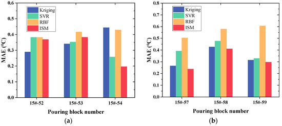
Figure 11.
Comparison of MAE based on different models. (a,b) describe the comparison results for C35 and C40 concrete, respectively.
As can be seen in Figure 11, the inversion accuracy of the ISM is higher than that of the individual surrogate models for all the pouring blocks except for 15#-52 and 15#-53. The average MAE for C35 and C40 concrete were calculated as shown in Table 5.
Table 5.
Comparison of average MAE based on different models (°C).
It can be seen that the inversion accuracy of ISM is better than all the individual models, with the closest result given by the Kriging model, and the worst by the RBF model. Compared with the Kriging, SVR, and RBF model, the MAE based on ISM reduces by 8.45%, 3.93% and 20.85%, respectively for C35 concrete, and by 6.53%, 23.82% and 44.43%, respectively for C40.
Compared to the other surrogate models, ISM increases the time taken to calculate the weights as well. For a dataset with a sample size of 60, the time cost to determine the weights is about 50 min. Furthermore, it takes one hour to execute the finite element model in this paper on an ordinary computer, while a trained ISM only needs a few seconds. Based on the parameter setting of the Jaya algorithm in this paper, 8000 times are required to execute the finite element model by directly invoking it for inversion analysis, while the proposed method only needs only 60 + 10 times, resulting in an approximately 111.7-fold increase in computational efficiency. In summary, the method proposed in this paper still maintains a massive advantage in computational efficiency.
3.5. Discussion
Previous studies have already demonstrated the significance of thermal parameter inversion on the dynamic simulation of temperature fields during the construction period. However, it has been a challenge to reconcile the efficiency and accuracy of the inversion analysis. To solve this problem, this article proposed a thermal parameter inversion method using uniform design, ISM, and Jaya optimization algorithm. This approach is applied to the concrete thermal parameters inversion for two strength grades of an extra-high arch dam. Its effectiveness was verified by evaluating the ISM’s predictive capability, inversion accuracy, and inversion efficiency.
Introducing the SBO method in thermal parameter inversion aims to enhance the efficiency of the process, particularly concerning intricate temperature analysis models. Consequently, the proposed methodology in this paper holds a stronger advantage in computational efficiency compared to direct inversion methods based on GA [11], DE [12], PSO [13], and WOA [14]. Furthermore, compared to the inversion methods based on individual surrogate models in Ref [20,21,22], the proposed method sacrifices a small amount of computational efficiency and does not have an absolute advantage in inversion accuracy. However, it enhances the robustness of the surrogate model and avoids the negative effects of inappropriate model selection. For example, in this study, although the accuracy of the inversion results based on the Kriging model is close to that of the ISM, as shown in Table 5, the problem is that we do not know beforehand whether using Kriging would obtain better results. The ISM, to some extent, avoids this issue.
In summary, the method proposed in this paper advances the balance between inversion accuracy and efficiency compared to traditional methods. It provides a simple and effective strategy for obtaining the thermal properties of concrete accurately and efficiently. Additionally, this method has potential applications for the thermal analysis of massive concrete structures, such as bridge piers and pumping stations.
4. Conclusions and Future Work
The inversion of concrete thermal parameters is crucial for the thermal analysis of dams. Previous methods using optimization algorithms to identify parameters directly have huge computational costs, while methods based on individual surrogate models suffer from difficulties in model selection. This study employs an ISM combined with the Jaya optimization algorithm to invert multiple thermal parameters of concrete dams. This approach can efficiently and accurately identify the thermal parameters of dams. Three machine learning algorithms, Kriging, SVR and RBF, were used to construct the ISM, which is a new attempt to invert the thermal parameters of concrete. The prediction performance is validated with multiple sample sets, showing that the ISM can combine the advantages of several individual surrogate models and is more robust than the sub-models in fitting the mapping relationship between the concrete thermal parameters and the temperature responses. Then, the proposed method was applied to identify multiple thermal parameters of two strength grades of concrete in an arch dam. The results show that the calculated temperatures based on the inversion tend to be consistent with the monitored temperatures, with MAE of 0.32 °C and 0.31 °C, respectively, reflecting the thermal properties of concrete under natural pouring conditions, which verifies the reliability of the inversion results. Subsequently, the inversion accuracy using the ISM and the individual surrogate model were compared. Compared with Kriging, SVR, and RBF models, the ISM, which provides more accurate inversion results, reduces errors by 8.45%, 3.93%, and 20.85%, respectively for C35 concrete, and by 6.53%, 23.82%, and 44.43%, respectively for C40 concrete. On top of that, it also retains the advantage of high computational efficiency. Comprehensively, the proposed method demonstrates a more balanced inversion accuracy and efficiency.
However, some limitations are equally noteworthy. The sample set in this paper was generated in a single pass, which may make it difficult to obtain sufficient critical information with a small sample size. Therefore, there is great potential to introduce a sequential sampling strategy in the experimental design of future studies.
Author Contributions
Conceptualization, F.W. (Fang Wang), C.Z. and Y.Z.; data curation, H.Z.; methodology, F.W. (Fang Wang) and C.Z.; software, F.W. (Fang Wang) and H.Z.; validation, Z.L. and F.W. (Feng Wang); formal analysis, F.W. (Fang Wang); funding acquisition, F.W. (Fang Wang) and H.Z.; project administration, Y.Z.; visualization, E.A.S.; Writing—Original draft, F.W. (Fang Wang); Writing—Review and editing, C.Z., Y.Z. and A.Z. All authors have read and agreed to the published version of the manuscript.
Funding
This research work was supported by the Research Fund for Excellent Dissertation of China Three Gorges University (Grant No. 2020BSPY013), the Youth Fund project of the National Natural Science Foundation of China (No. 52109157), and the Open Foundation of the Key Laboratory of Hydro-power Engineering Construction and Management of Hubei Province (Grant No. 2019KSD08).
Institutional Review Board Statement
Not applicable.
Informed Consent Statement
Not applicable.
Data Availability Statement
Not applicable.
Conflicts of Interest
The authors declare no conflict of interest.
References
- Chu, I.; Lee, Y.; Amin, M.N.; Jang, B.; Kim, J. Application of a thermal stress device for the prediction of stresses due to hydration heat in mass concrete structure. Constr. Build. Mater. 2013, 45, 192–198. [Google Scholar] [CrossRef]
- Peng, H.; Lin, P.; Xiang, Y.; Hu, J.; Yang, Z. Effects of Carbon Thin Film on Low-Heat Cement Hydration, Temperature and Strength of the Wudongde Dam Concrete. Buildings 2022, 12, 717. [Google Scholar] [CrossRef]
- Alamayreh, M.I.; Alahmer, A.; Younes, M.B.; Bazlamit, S.M. Pre-Cooling Concrete System in Massive Concrete Production: Energy Analysis and Refrigerant Replacement. Energies 2022, 15, 1129. [Google Scholar] [CrossRef]
- Conceição, J.; Faria, R.; Azenha, M.; Miranda, M. A new method based on equivalent surfaces for simulation of the post-cooling in concrete arch dams during construction. Eng. Struct. 2020, 209, 109976. [Google Scholar] [CrossRef]
- Wang, Z.; Xiao, J.; Shi, Z.; Zhang, B. Influence of Longitudinal Joint Setting and Synchronous Cooling Zone on High Altitude Region’s Dam Construction. Appl. Sci. 2022, 12, 7380. [Google Scholar] [CrossRef]
- Mirković, U.; Kuzmanović, V.; Todorović, G. Long-Term Thermal Stress Analysis and Optimization of Contraction Joint Distance of Concrete Gravity Dams. Appl. Sci. 2022, 12, 8163. [Google Scholar] [CrossRef]
- Ouyang, J.; Chen, X.; Huangfu, Z.; Lu, C.; Huang, D.; Li, Y. Application of distributed temperature sensing for cracking control of mass concrete. Constr. Build. Mater. 2019, 197, 778–791. [Google Scholar] [CrossRef]
- Gioda, G. Indirect identification of the average elastic characteristics of rock masses. In Proceedings of the International Conference on Structural Foundations on Rock, Sydney, Australia, 7–9 May 1980; pp. 65–73. [Google Scholar]
- Asaoka, A.; Matsuo, M. An inverse problem approach to the predication of multi-dimensional consolidation behavior. Soils Found. 1984, 24, 49–62. [Google Scholar] [CrossRef]
- Anandarajah, A.; Agarwal, D. Computer-aided calibration of a soil plasticity model. Int. J. Numer. Anal. Methods 1991, 15, 835–856. [Google Scholar] [CrossRef]
- Ding, J.; Chen, S. Simulation and feedback analysis of the temperature field in massive concrete structures containing cooling pipes. Appl. Therm. Eng. 2013, 61, 554–562. [Google Scholar] [CrossRef]
- Xu, J.; Shen, Z.; Yang, S.; Xie, X.; Yang, Z. Finite element simulation of prevention thermal cracking in mass concrete. Int. J. Comput. Sci. Math. 2019, 10, 327–339. [Google Scholar] [CrossRef]
- Wang, F.; Zhou, Y.; Zhao, C.; Zhou, H.; Chen, W.; Tan, Y.; Liang, Z.; Pan, Z.; Wang, F. Thermal parameter inversion for various materials of super high arch dams based on hybrid particle swarm algorithm method. J. Tsinghua Univ. (Sci. Technol.) 2021, 61, 747–755. [Google Scholar]
- Hu, Y.; Bao, T.; Ge, P.; Tang, F.; Zhu, Z.; Gong, J. Intelligent inversion analysis of thermal parameters for distributed monitoring data. J. Build. Eng. 2023, 68, 106200. [Google Scholar] [CrossRef]
- Viana, F.A.C.; Haftka, R.T.; Steffen, V. Multiple surrogates: How cross-validation errors can help us to obtain the best predictor. Struct. Multidiscip. Optim. 2009, 39, 439–457. [Google Scholar] [CrossRef]
- Das, R.; Soulaimani, A. Non-Deterministic Methods and Surrogates in the Design of Rockfill Dams. Appl. Sci. 2021, 11, 3699. [Google Scholar] [CrossRef]
- Tullu, A.; Lee, B.; Hwang, H. Surrogate Model Based Analysis of Inter-Ply Shear Stress in Fiber Reinforced Thermoplastic Composite Sheet Press Forming. Appl. Sci. 2020, 10, 5499. [Google Scholar] [CrossRef]
- Wang, Y.; Zhao, R.; Liu, Y.; Chen, Y.; Ma, X. Shape Optimization of Single-Curvature Arch Dam Based on Sequential Kriging-Genetic Algorithm. Appl. Sci. 2019, 9, 4366. [Google Scholar] [CrossRef]
- Chen, Z.; Zhao, Q. A Dynamic Model Updating Method with Thermal Effects Based on Improved Support Vector Regression. Appl. Sci. 2021, 11, 8025. [Google Scholar] [CrossRef]
- Pei, L.; Chen, J.K.; Wu, Z.Y.; Li, Y.L.; Zhang, H. Response surface genetic algorithm of back analysis of concrete thermal parameters. Mater. Res. Innov. 2015, 19, S8-840–S8-845. [Google Scholar] [CrossRef]
- Zhou, H.; Zhou, Y.; Zhao, C.; Wang, F.; Liang, Z. Feedback Design of Temperature Control Measures for Concrete Dams based on Real-Time Temperature Monitoring and Construction Process Simulation. KSCE J. Civ. Eng. 2018, 22, 1584–1592. [Google Scholar] [CrossRef]
- Wang, F.; Zhou, H.; Zhou, Y.; Zhao, C.; Seman, E.A.; Gong, P. Thermal Parameters Inversion Method for Concrete Dam Based on Optimal Temperature Measuring Point Selecting. Math. Probl. Eng. 2022, 2022, 4677344. [Google Scholar] [CrossRef]
- Acar, E.; Rais-Rohani, M. Ensemble of metamodels with optimized weight factors. Struct. Multidiscip. Optim. 2009, 37, 279–294. [Google Scholar] [CrossRef]
- Cheng, K.; Lu, Z. Structural reliability analysis based on ensemble learning of surrogate models. Struct. Saf. 2020, 83, 101905. [Google Scholar] [CrossRef]
- Xiao, T.; Park, C.; Ouyang, L.; Ma, Y. An active learning Bayesian ensemble surrogate model for structural reliability analysis. Qual. Reliab. Eng. Int. 2022, 38, 3579–3597. [Google Scholar] [CrossRef]
- Fang, J.; Gao, Y.; Sun, G.; Xu, C.; Li, Q. Fatigue optimization with combined ensembles of surrogate modeling for a truck cab. J. Mech. Sci. Technol. 2014, 28, 4641–4649. [Google Scholar] [CrossRef]
- Zhou, S.; Lu, L.; Xu, B.; He, J.; Xia, D. Performance Optimization Design of Diagonal Flow Fan Based on Ensemble of Surrogates Model. Appl. Sci. 2022, 12, 9732. [Google Scholar] [CrossRef]
- Yin, J.; Tsai, F.T.C. Bayesian set pair analysis and machine learning based ensemble surrogates for optimal multi-aquifer system remediation design. J. Hydrol. 2020, 580, 124280. [Google Scholar] [CrossRef]
- Li, J.; Wu, Z.; Lu, W.; He, H. Simultaneous identification of the number, location and release intensity of groundwater contamination sources based on simulation optimization and ensemble surrogate model. Water Supply 2022, 22, 7671–7689. [Google Scholar] [CrossRef]
- Bofang, Z. Thermal Stresses and Temperature Control of Mass Concrete; Butterworth-Heinemann: Oxford, UK, 2013. [Google Scholar]
- Li, Y.F.; Ng, S.H.; Xie, M.; Goh, T.N. A systematic comparison of metamodeling techniques for simulation optimization in Decision Support Systems. Appl. Soft Comput. 2010, 10, 1257–1273. [Google Scholar] [CrossRef]
- Kianifar, M.R.; Campean, F. Performance evaluation of metamodelling methods for engineering problems: Towards a practitioner guide. Struct. Multidiscip. Optim. 2020, 61, 159–186. [Google Scholar] [CrossRef]
- Goel, T.; Haftka, R.T.; Shyy, W.; Queipo, N.V. Ensemble of surrogates. Struct. Multidiscip. Optim. 2007, 33, 199–216. [Google Scholar] [CrossRef]
- Su, H.; Wen, Z.; Zhang, S.; Tian, S. Method for Choosing the Optimal Resource in Back-Analysis for Multiple Material Parameters of a Dam and Its Foundation. J. Comput. Civil. Eng. 2016, 30, 4015060. [Google Scholar] [CrossRef]
- Wang, J.; Xia, C.; Fan, X.; Cai, J. Research on the Influence of Tractor Parameters on Shift Quality, Based on Uniform Design. Appl. Sci. 2022, 12, 4895. [Google Scholar] [CrossRef]
- Song, X.; Lv, L.; Sun, W.; Zhang, J. A radial basis function-based multi-fidelity surrogate model: Exploring correlation between high-fidelity and low-fidelity models. Struct. Multidiscip. Optim. 2019, 60, 965–981. [Google Scholar] [CrossRef]
- Le, T. Surrogate Neural Network Model for Prediction of Load-Bearing Capacity of CFSS Members Considering Loading Eccentricity. Appl. Sci. 2020, 10, 3452. [Google Scholar] [CrossRef]
- Venkata Rao, R. Jaya: A simple and new optimization algorithm for solving constrained and unconstrained optimization problems. Int. J. Ind. Eng. Comp. 2016, 7, 19–34. [Google Scholar] [CrossRef]
- Kang, F.; Li, J.; Dai, J. Prediction of long-term temperature effect in structural health monitoring of concrete dams using support vector machines with Jaya optimizer and salp swarm algorithms. Adv. Eng. Softw. 2019, 131, 60–76. [Google Scholar] [CrossRef]
- Kang, F.; Liu, X.; Li, J.; Li, H. Multi-parameter inverse analysis of concrete dams using kernel extreme learning machines-based response surface model. Eng. Struct. 2022, 256, 113999. [Google Scholar] [CrossRef]
- Liang, Z.; Zhao, C.; Zhou, H.; Liu, Q.; Zhou, Y. Error correction of temperature measurement data obtained from an embedded bifilar optical fiber network in concrete dams. Measurement 2019, 148, 106903. [Google Scholar] [CrossRef]
- Zhou, Y.; Liang, C.; Wang, F.; Zhao, C.; Zhang, A.; Tan, T.; Gong, P. Field test and numerical simulation of the thermal insulation effect of concrete pouring block surface based on DTS. Constr. Build. Mater. 2022, 343, 128022. [Google Scholar] [CrossRef]
- Kim, D.; Lee, S.; Lee, J. Data-Driven Prediction of Vessel Propulsion Power Using Support Vector Regression with Onboard Measurement and Ocean Data. Sensors 2020, 20, 1588. [Google Scholar] [CrossRef] [PubMed]
- Jena, P.R.; Majhi, B.; Majhi, R. Estimating Long-Run Relationship between Renewable Energy Use and CO2 Emissions: A Radial Basis Function Neural Network (RBFNN) Approach. Sustainability 2022, 14, 5260. [Google Scholar] [CrossRef]
- Bhattacharyya, B. Uncertainty quantification of dynamical systems by a POD–Kriging surrogate model. J. Comput. Sci.-Neth. 2022, 60, 101602. [Google Scholar] [CrossRef]
Disclaimer/Publisher’s Note: The statements, opinions and data contained in all publications are solely those of the individual author(s) and contributor(s) and not of MDPI and/or the editor(s). MDPI and/or the editor(s) disclaim responsibility for any injury to people or property resulting from any ideas, methods, instructions or products referred to in the content. |
© 2023 by the authors. Licensee MDPI, Basel, Switzerland. This article is an open access article distributed under the terms and conditions of the Creative Commons Attribution (CC BY) license (https://creativecommons.org/licenses/by/4.0/).