Featured Application
The model and analysis results established in this paper can be used for dynamic analyses of the autonomous driving control of articulated steering vehicles, as well as for the design of hybrid or pure electric power articulated steering vehicles.
Abstract
Articulated steering vehicles (ASVs), with brilliant maneuverability and efficiency, are being widely applied in mining, construction, agriculture, and forestry. However, their special structures result in them having complex dynamic characteristics, but there are no reliable models for further research. This study established a simulation platform with the dynamic model of ASVs, where the subsystems of the power train, steering systems, tires, and frames were also included. The dynamic model was validated with field test data of typical working cycles, in which the focus was on longitudinal and lateral motions and the characteristics of steering and power train systems. Then, the distribution of hydraulic and drive power was revealed using the simulation platform and test data. For a load–haul–dump (LHD) vehicle with a 6 m3 capacity, the maximum power of the system was about 289 kW; the power of the motor accounted for the majority of the power at the beginning stage of loading, being about 74%, and then the hydraulic power dominated in the later stage of loading. During the transport stage, the power of the motor accounted for about 79% of the total power. Finally, the influence of the dynamic parameters on lateral and longitudinal motions was analyzed based on the validated platform.
1. Introduction
Articulated steering vehicles (ASVs), which include different vehicles, such as load–haul–dump (LHD) vehicles [1], wheel loaders [2,3], and dump trucks [4], are widely used in underground mines, the construction industry, and forestry [5], as shown in Figure 1. Their special steering structure brings about excellent maneuverability and efficiency advantages, but it also causes complex, dynamic problems.
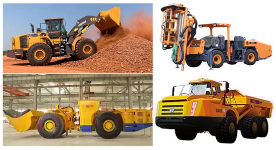
Figure 1.
Typical applications of ASVs.
Two frames can cooperatively rotate along the vertical direction during steering and non-steering maneuvers; however, relative oscillation is inevitable and will cause the problems of sideslip and handling stability, i.e., running like a snake. In addition, ASVs always run and work in harsh environments, such as in underground mines, with a high humidity and high temperatures, and in dusty construction sites. Autonomous ASVs [6] are urgently needed for these driving [7] and working processes [1,8]. Thus far, these involved needs and problems have been solved with reliable models and via further research on commercial vehicles, as these solutions are also applicable to ASVs [9]. For example, a path that follows an autonomous function is based on the kinematic model of target vehicles. Additionally, lateral stability control is based on the dynamic model [10] of target vehicles [11].
However, the kinematics and dynamics of ASVs are quite different from those of conventional commercial vehicles. For ASVs, the structure contains two frames, which are articulated with each other, and each frame is equipped with an axle. They are usually all-wheel drive in order to obtain an excellent power performance. The steering function is realized by the articulated motion of the frames in the vertical direction. During the process of steering, the frames form a specific geometric relationship, and the kinematic model of ASVs can be obtained by assuming no slip [12]. However, lateral slip is always inevitable during the steering process. Oscillation, snake-like running, jack-knifing, and related problems are considered to be dynamic instability. Although some models could be used to analyze the stability of ASVs, the transient characteristics of the steering system have not been covered. He et al. [13] researched the stability of ASVs based on a two-degree-of-freedom (DOF) and a three-DOF model, in which the difference of the two models was the yaw freedom of frames. The results stated that the leakage of hydraulic fluid affected stability in different modes of instability. Therefore, the impact of the steering system on dynamic responses is particularly critical, and the model should be detailed.
The steering system of an ASV is usually powered by a hydraulic cylinder, which is controlled by a hydraulic valve. The model involves the coupling of a hydraulic system and the connected frames. Gao et al. [14] developed a 12-DOF model of ASVs with Adams/View software, in which the detailed hydrostatic steering control unit was involved. The instability of snaking and oscillation was confirmed, and improvements were made with the yaw moment and driving force distribution control. Although this research mainly focused on lateral responses, the validation also concentrated on lateral motions. The research of [15] indicated that the lateral response also depended on longitudinal velocity ranges. In addition, the valve-controlled steering system is more universal. Therefore, a universally applicable model of ASVs should be presented holistically [16], and the validation of the model should be performed comprehensively [17].
Although traditional diesel-engine-driven ASVs provide excellent power and mobility, exhaust emissions are inevitable. In addition to the increasing cost of fuel, the requirement of environmental quality has also eliminated the usage of this type of ASV. Such as in underground mines, many pieces of ventilation equipment are needed to deal with the emissions of ASVs, i.e., of LHD vehicles, articulated trucks, drilling rigs, and so on. Some plug-in ASVs have been used in the working faces of underground mines; although the power was guaranteed by the towed cable, the mobility of the ASVs was severely restricted [18].
In order to address emission problems, the power of ASVs was improved with hybrid or pure electric power structures [19]. For hybrid power ASVs, the diesel engine is used to drive the generator, and the battery, supercapacitor, or both are used to store the energy of the power system [20]. For pure electric power ASVs, only the battery and some auxiliary accumulators are used to provide the energy, and the replacement or charging of the battery is executed after the power is exhausted [21]. The driving power of the motor and the hydraulic power of the working mechanism must be satisfied no matter which structure is adopted. The average power during the working cycle is not high, while the instantaneous power is very high, especially during the loading process. The driving and working mechanism power can be used to cover the bucket resistance force during the loading process. Therefore, the power distributions of ASVs are very important for the proper design of the power system and the energy management system. Many ASVs have been used in underground mines, where LHD vehicles are the most common [22]. LHD vehicles possess the most complex and changeable working conditions and determine the production efficiency of the whole mine [23].
Based on the above-mentioned problems and research studies, this article establishes a simulation platform of ASVs with the dynamic model. Additionally, the power distribution of an ASV is uncovered using the platform and test data of a typical working cycle. The main contributions are summarized as follows:
(1) An ASV simulation platform is established with the detailed dynamic model, and the dynamic responses of different systems in different directions are presented and validated.
(2) The power distribution of a typical ASV, i.e., an LHD vehicle, is uncovered based on the platform and test results from typical working cycles.
(3) The effects of the model parameters on the lateral and longitudinal dynamic responses are analyzed and presented.
The remainder of the work is structured as follows: The dynamic model of ASVs is presented in Section 2, and the subsystems of the frames, tires, the power train, and steering are included. In Section 3, an ASV field test is performed, and the validation results are presented. A discussion of the results is also included in this section. We conclude this paper in Section 4.
2. Dynamic Model of ASVs
2.1. Dynamic Model of Frames
LHD vehicles, which are typical ASVs and whose structure is shown in Figure 2, are usually used to transfer heavy goods or mine materials, and, thus, it is necessary to avoid the large vertical motion of the chassis as caused by any vertical load variations. Therefore, the suspension is normally absent in the chassis of an ASV. The dynamic motion of an ASV can be revealed with planar motion, i.e., the plane parallel to the ground. According to Figure 2, the tire forces, originating from the tires, act on the front and rear frames, and the hydraulic-driven steering system drives the two frames to fold around the articulated point. Therefore, the dynamic model of ASVs can be divided into three models, i.e., the model of the frames, the model of the tire forces, and the kinematic constraints of the frames.
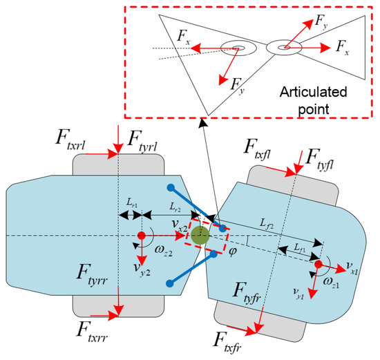
Figure 2.
Typical structure of ASV.
2.1.1. Model of Frames
The motion of the frames can be described with the two sets of frames: the ISO (the longitudinal forward direction of the vehicle is defined as the X axis, the vertical downward direction is defined as the Z axis, and the Y axis is in the right-hand coordinate system) front frame (X1Y1Z1) and the ISO rear frame (X2Y2Z2) [24]. The motion in the XY plane is focused on considering the target in this paper. According to Newton’s second law, the dynamic model of ASVs in the XY plane can be expressed as follows:
where subscripts 1 and 2 denote the front and rear frames, respectively; φ is the articulation angle; B is half of the wheel track; m1 and m2 are the masses of the front and rear frames, respectively; Iz1 and Iz2 are the moments of inertia in the z direction; Fx and Fy are internal forces at the central point; Fsxf, Fsyf, Fsxr, Fsyr, Mszf, and Mszr are the forces and moments caused by the steering cylinder; Ftxf, Ftyf, Ftxr, Ftyr, Ftxfl, Ftxfr, Ftxrl, and Ftxrr denote the front and rear tire forces in the x and y directions; Lf1 and Lr1 are the distances between the mass center of the front and the rear frames (as well as the corresponding axles), respectively; and Lf2 and Lr2 are the distances between the mass center of the front and the rear frames (as well as the central articulated point), respectively.
2.1.2. Model of Tire Forces
Many tire models have been developed for different conditions and purposes, including theoretical models, empirical models, and semi-empirical models [24]. In this paper, the brush model is used due to the conditions of ASVs and the purpose of this paper. The longitudinal force and the lateral force of the tires under the comprehensive working condition of the brush model can be expressed as
where Fx_ij—Fx_fl, Fx_fr, Fx_rl, and Fx_rr—is the force of the different wheels in the longitudinal direction; Fy_ij—Fy_fl, Fy_fr, Fy_rl, and Fy_rr—is the corresponding lateral force for the different wheels; and Cx and Cy are the corresponding stiffnesses.
The other correlation coefficients can be expressed as follows:
where the coefficient κ can be expressed as
where α is the tire slip angle, and η is the tire slip rate; thus, it can be expressed that
where the rolling radius, the angular speed, and the speed of the frames are denoted by rdij, ωij, and vxij, respectively. The corresponding speed of the two structures can be written as
The sideslip angle can be expressed as
2.1.3. Kinematic Constraints of Frames
According to Figure 2, the two frames are connected to each other at the central articulated point. The motions of the frames are related to each other in the longitudinal and lateral directions. The detailed constraints of the two frames in different directions can be given by
Additionally, the heading angles of the frames are constrained by the articulated angle, which is expressed as
where Ψ1 and Ψ2 are the heading angles of the front and rear frames.
The kinematic constraints in Equation (9) can be processed with differentiation, and the acceleration constraints can be obtained:
2.2. Model of Steering System
2.2.1. Hydraulic System
The steering maneuver of an ASV is performed with hydraulic cylinders, and the hydraulic cylinders are arranged on both sides of the articulated point [25]. The rod and rodless cavities of the two cylinders are connected crossly to obtain a cooperative steering moment, as shown in Figure 3a. A steering valve, with the pressure compensation in front of the spool, is used to control the direction of the steering, and its flow is decided by the control current. The articulated steering hydraulic system and the geometric relationship are shown in Figure 3b. Then, the flow and force balance equations of the two steering cylinders can be expressed as follows:
where the flow, volume, and pressure of the two chambers of the two cylinders are represented by Qij (i = L, R; j = 1, 2), Pij (i = L, R; j = 1, 2), and Vij (i = L, R; j = 1, 2), respectively. A1 and A2, as well as XR and XL, are the corresponding action areas and displacement values, respectively, whereas fs is the coefficient of dynamic friction.
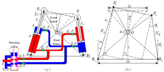
Figure 3.
The ASV steering system. (a) The hydraulic circuit of the steering system; (b) the geometric relationship of the system.
2.2.2. Kinematic Model
According to the geometric relationship of the steering system in Figure 3b, the forces of the cylinders act on the front and rear frames, and, thus, different angles are formed when the articulated angle φ changes, causing these angles to affect the action arm of the cylinders. The different angles between the cylinders and the frames can be expressed as
where γi and βi (i = 1, 2) denote the angles between the left and right cylinders and the front and rear frames, respectively. Additionally, the length of the cylinders XL and XR and the intermediate variables YL and YR can be expressed as
According to Equations (12)–(17), the force and moment acting on the front and rear frames can be obtained, which can be expressed as follows:
Then, by substituting Equations (3)–(11) and (18) into Equations (1) and (2), the dynamic model of ASVs in the XY plane can be obtained. The tire force in the lateral and longitudinal directions originates from the steering maneuver and the power train system. The model of the power train is given in the next subsection.
2.3. Model of the Power Train
The target ASV, an LHD vehicle, is driven with an electric motor, and the relationship between the main components in the power train is shown in Figure 4. The arrangements of the front and rear driving systems are the same, and two driven motors are used in the power system. The characteristics of the motor are shown in Figure 5, and the maximum speed and torque are 3000 r/min and 2500 Nm, respectively, with a maximum power of 200 kW. According to the curve in Figure 5, during 0~500 r/min, the maximum torque remains constant, and the power gradually increases during this period.
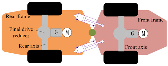
Figure 4.
Main components of ASV power train.
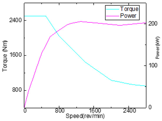
Figure 5.
External characteristics of driven motor.
An LHD vehicle always runs in a narrow area, and its turning radium is very short. During steering maneuvers, the speed difference between the inner and outer wheels is very large; therefore, the differential mechanism is necessary for the drive axle of this ASV. According to this principle, the model of the differential mechanism can be expressed as
where Jin, Jl, and Jr are the rotational inertia of the input axle, left output axle, and right output axle, respectively; Tin, Tl, and Tr and ωin, ωl, and ωr are the corresponding torques and angular velocities. c denotes viscous damping. Tin_r, Tl_r, and Tr_r are the resistance torques of the different axles.
The out torque of the differential mechanism is transmitted to the wheel with a half axis, and the model can be given by
where Tc is the clutch torque, and η is the gear ratio, which is 55 in this LHD power train.
The final drive torque in the wheel overcomes the rolling resistance force and braking force to produce the longitudinal driving force, and the detailed model can be expressed as
where Iw is the rotational inertia of the wheel, and Tij (i = f, r; j = l, r) is the corresponding driving torque. fr is the rolling resistance force, which can be expressed as
3. Results and Discussion
After determining the process in Section 2, we established a simulation platform with the dynamic model of ASVs using Matlab/Simulink software. The system contained a power train system, a steering system, a braking system, and the lateral and longitudinal dynamic responses of the frames. The inputs were the signals of the acceleration pedal, the braking pedal, and the steering handle, just as in a real LHD vehicle. The simulation interval was set as 0.01 s, i.e., 100 Hz, and the parameters are shown in Table 1.

Table 1.
Main involved parameters.
In order to validate the embedded dynamic model, we performed a field test on a load–haul–dump vehicle. A diagram of the field test system is shown in Figure 6. The states of the frames, steering system, and power train were recorded. The data involved during the field test, including velocity, angular velocity, articulated angle data, torque, and pressure, were recorded, and the sample rate was set to 100 Hz. An LMS SCADAS (①, SCM05) was used to record the data during the field test. Two inertial measurement units (IMUs) (②, ③, SC-AHRS-200A) were installed in the front and rear frames. Two kinds of encoders were used to measure the articulated angle of the frame (④, MIRAN WOA-C) and the speed of transmission (⑤, SCHMEASAL IFL 5-18M-10P). Pressure sensors (⑥, AE-H) were installed to measure the pressure of the steering system and the braking system. The acceleration pedal and the state of the motors were recorded in the controller of the LHD vehicle.
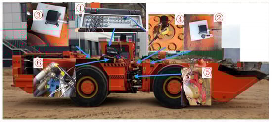
Figure 6.
Field test system of target ASV.
The obtained input signal of the test vehicle was input into the simulation model, and the responses were compared with the test results to validate the model. For the ASV, off-road conditions were used for the running ground in order to examine a compacted earth road, with a standard road roughness of level E. If the road conditions are not modeled accurately, then differences between the field test and simulation are inevitable.
3.1. Longitudinal and Lateral Responses
The input of the acceleration and braking pedal is shown in Figure 7a, and a comparison of the longitudinal velocity results is shown in Figure 7b. According to the results in Figure 7, the test vehicle accelerated with small and intensive maneuvers between approximately 3 and 8 s, and fast acceleration occurred at 10~20 s and 25~39 s. The pressure of the braking system remained constant, around 10.3 MPa, when there was no braking motion, and it decreased rapidly to 4.1 MPa when the brake was triggered around 21~24 s. According to the results in Figure 7b, the longitudinal velocity in the field test and the simulation varied for the same trend and amplitude. The two results almost coincided during the acceleration and braking maneuvers, and only minor differences appeared during the free-running period, i.e., 39~41.8 s, while the same difference also occurred around 9.2~10.1 s. This error was brought on by the rolling resistance force model. The used resistance force model was established based on the paved road condition, while the test road was an unpaved road. The maximum velocity of the test was about 7.1 km/h, and the corresponding result was about 6.9 km/h. Therefore, the model can reveal the longitudinal dynamics of an ASV.
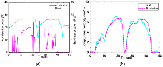
Figure 7.
Longitudinal input and responses. (a) Input signal; (b) longitudinal velocity comparison results.
The lateral responses were analyzed with the yaw velocity of the two frames during steering maneuvers. Additionally, the longitudinal velocity was kept constant during the test to avoid the effects of acceleration and braking. The yaw velocity results are shown in Figure 8. According to the results in Figure 8, the yaw velocity of the two frames varied differently during the unsteady steering process and varied identically during the steady process, where the variations in the tests were −13~11°/s and −14~9°/s, respectively, and the corresponding results of the simulation varied between −15 and 10°/s and between −15 and 17°/s. Although the maximum values were different, the trends were almost the same during the steering process, and the transient peak difference only existed for a moment according to the detailed graphs in Figure 8.
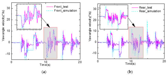
Figure 8.
Lateral responses. (a) Front frame responses; (b) rear frame responses.
In addition, around 4.5~6 s, the steady yaw velocity was different, which was caused by the longitudinal velocity difference between the test and the simulation. According to the kinematic model of ASVs, the steady yaw velocity is decided by the longitudinal velocity and the articulated angle. Additionally, the frequent fluctuation of the curves in the test also indicated the yaw oscillation after the steering process. In contrast, the simulation results were more smooth. During the field test, the running road was uneven, and the constant external force caused the variation. The mean values of the simulation and the test coincided well during the steady steering process.
3.2. Dynamic Responses of Steering System
The steering system of an LHD vehicle is essential for establishing its excellent maneuverability, as the system contains the hydraulic power components, i.e., steering cylinders. The variation in the articulated angle is the result of steering. Therefore, we focused on the dynamic responses of the steering system based on the articulated angle and pressure of the steering cylinder. The articulated angle results are shown in Figure 9. Figure 9a shows the control current of the main valve, and the signal, including the continuous and directional steering operations, was input into the simulation model. According to the comparison results in Figure 9b, the angle varied between −10° and 5°, and the simulation result was the same as the test result. Only a tiny difference occurred after the steering, which was about 0.3° according to the detailed figure. In addition, according to the results in Figure 8, the two frames oscillated after the steering maneuver, and the fluctuation of the articulated angle also supports the results. However, the angle did not fluctuate dramatically, which meant that the relative and cooperative oscillations of the two frames occurred at the same time.
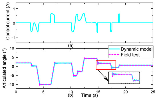
Figure 9.
Articulated angle results. (a) Steering signal; (b) articulated angle.
According to the structure of the hydraulic pipes in Figure 3, the rodless chamber of the left cylinder is connected to the rod chamber of the right cylinder and vice versa for the other chambers. Therefore, only the pressures of the two chambers obviously varied. Additionally, we compared the results of the two chambers and found that the trends and amplitudes were almost same. Therefore, only the rodless chamber pressure of the left steering cylinder, shown in Figure 10, was analyzed. As it can be seen, the steering pressure varied between 0.1 and 14 MPa. During the steady steering process, the valve was closed, the pressure oil was cut off, and all chambers of the cylinders were closed. The pressure might remain constant at a different level, which is reasonable and independent of the dynamic model accuracy at this stage. During the steering process, between 10 and 13 s, the simulation results coincided well with the test results, causing the small trend according to the detailed figure. The results of the analysis indicate that the established simulation platform can simulate the dynamic responses of the steering system well.
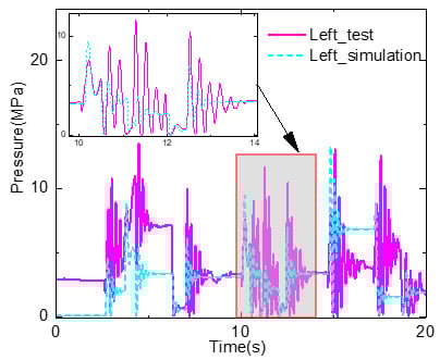
Figure 10.
Pressure results of steering system.
3.3. Power Train Results
In order to validate the power train model, we recorded the torque information of the front and rear motors during the test, and the torque of the two motors was the same; thus, only the front motor is shown and compared with the simulation results in Figure 11. As it can be seen, the maximum torque was about 780 Nm during the presented test interval, and the maximum torque was about 650 Nm in the simulation, meaning that they occurred at the same time. Additionally, a large difference occurred during the slow reduction stage, i.e., at 11~17 s and 26~29.5 s. In the simulation model, the motor was considered to be a table with two parameters, the acceleration pedal and speed. The resulting torque might be slightly different from the actual characteristic of the motor. During the other stages, the simulation and test results coincided well, especially during the low-torque stages.
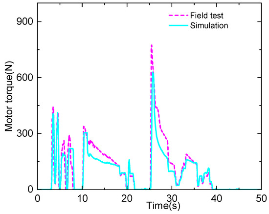
Figure 11.
Torque result of driving motor.
Not only does the power train of an LHD vehicle provide the power of the driving and steering system, but it also provides the power of the working mechanism, which is normally powered by hydraulic oil like the steering system. Meeting the power demand is essential to the productivity of an LHD vehicle, and, thus, the power demand should be uncovered. In order to analyze the power distribution of a typical working cycle, we recorded the pressure and flow of the steering pump and working pump, and the current and voltage of the driving motor during three working cycles, in which the short-running, loading, running, dumping, and running-back processes were included.
Then, the power of the motor and hydraulic system was calculated, and the total power was obtained via the sum of the two parts, as shown in Figure 12. For the first working cycle, during 0~30 s, the ASV was run to load the mining material, and then it transported the material to the dump point between 30 and 75 s. The model validation was performed with the data from this process. The model-based calculation results of the motor power and hydraulic steering power also indicate correctness. The dump and return processes occupied the time interval of 75~125 s.
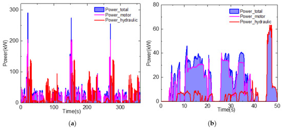
Figure 12.
Power distribution of typical working cycle: (a) global distribution; (b) power distribution in running condition.
The data of the model validation were extracted in the interval of 30~80 s, and the power distribution is shown in Figure 12b. As it can be seen from the results in Figure 12a, the maximum power during the typical cycle varied from 260 kW to 289 kW, and the motor power accounted for a large part, about 203 kW. When the ASV loaded the material, the vehicle was driven to insert the bucket tip deeper into the pile, and the motor power was used to cover the resistance force during the process. For the interval of model validation, which is 0~45 s in Figure 12b, the maximum power was about 48 kW, and the hydraulic power was the steering power, which was less than 10 kW.
Detailed information of the load and dump processes is shown in Figure 13a,b. For the results in Figure 13a, after the insertion of the bucket tip, the hydraulic power raised sharply due to the retraction of the bucket [26]. The motion needed to cover the stacking resistance force of the material pile. After that, i.e., the time after 23 s, the hydraulic power raised again, but it was less than 150 kW. During this process, the bucket and boom cylinders were cooperatively driven to load the material. In the dump process, the bucket needed to firstly be lifted and tilted. Then, the bucket returned to the original place with the cooperative control between the bucket and boom cylinders. Therefore, multiple fluctuations in the hydraulic power were involved. The maximum power of the dump process was less than 82 kW according to Figure 13b. After the dump process, the LHD vehicle was driven back to the load point, and the motor power and hydraulic power, i.e., the steering system, dominated in this region.
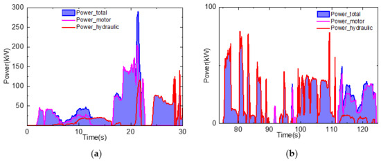
Figure 13.
Power distribution of loading and dumping conditions: (a) loading condition distribution; (b) dumping condition distribution.
3.4. Model-Based Analysis
In the dynamic model of these vehicles, the motions in the lateral and longitudinal directions depend on the tire force. Therefore, the parameters of the tire affected the dynamic responses of the vehicles significantly [27]. The model of ASVs also confirmed this characteristic. However, the tires used in ASVs are usually off-road tires, and the parameters cannot be obtained with a test rig, as even the producer cannot provide the related parameters. Therefore, the method of trial and error with the test data was deemed suitable. We obtained the proper stiffness of the tires with the longitudinal velocity and torque data, and the results are presented in Figure 14. Additionally, the order of magnitude of tire stiffness can be estimated with the mass of the frames. According to Figure 14a, when the longitudinal stiffness was too small, the acceleration and braking processes were insensitive, which meant that the tires could not provide enough longitudinal force. The results in Figure 14b indicate that the lateral stiffness affected the dynamic responses of the steering process. When the lateral stiffness was too large, the final yaw velocity and the resulting heading angle were also too large; i.e., oversteering occurred in the ASV. In contrast, when the value was too small, the ASV could not steer with the proper yaw velocity; i.e., it understeered. The tires were too soft to provide enough lateral force. The simulation results show that the articulated angle was not affected, which meant that the lateral slip of the tires occurred.

Figure 14.
Model-based analysis results: (a) effects of longitudinal stiffness of tires; (b) effects of lateral stiffness of tires.
4. Conclusions
This study established a simulation platform for ASVs with a dynamic model. In the dynamic model, the power train, steering, tires, and frames were considered, and the tire parameters were obtained via trial and error. The field test of one type of ASV, an LHD vehicle, was performed over a typical working cycle. The longitudinal responses coincided well for the acceleration and braking maneuvers, with an error of less than 0.5 km/h, and the large error that occurred during the free-running period was about 1.2 km/h. The lateral responses of the simulation and test all indicated oscillation in the yaw motion. The oscillation was more severe owing to the real complex force in the field test. The response of the steering system model was very accurate, with the error of the articulated angle being less than 0.3° in about a 15° variation range. For the power distribution of the LHD vehicle, the maximum power of the system was about 289 kW; the power of the motor accounted for the majority of the power at the beginning stage of loading, being about 74%, but then the hydraulic power dominated in the later stage of loading. During the transport stage, the power of the motor accounted for about 79% and the hydraulic power accounted for about 21% of the total power. The power of the system was less than 82 kW. In the future, the energy storage system will be embedded into the platform. The simulation platform can be used for dynamic control and energy management research.
Author Contributions
Conceptualization, L.G. and Y.D.; methodology, L.G. and J.Z.; software, L.G. and Y.D.; validation, L.G., Y.D. and J.Z.; data curation, Y.D.; writing—original draft preparation, L.G. and Y.D.; writing—review and editing, L.G.; visualization, L.G. and J.Z.; supervision, L.G.; project administration, L.G.; funding acquisition, L.G. All authors have read and agreed to the published version of the manuscript.
Funding
This research was funded by the National Natural Science Foundation of China (grant number 52104159), the fellowship of China Postdoctoral Science Foundation (grant No. 2021M690360), the Postdoctoral Science Foundation of Shunde Innovation School (grant No. 2021BH013), and the Special fund for scientific and technological innovation in Foshan (grant No. BK22BE018).
Institutional Review Board Statement
Not applicable.
Informed Consent Statement
Not applicable.
Data Availability Statement
Not applicable.
Conflicts of Interest
The authors declare no conflict of interest.
References
- Tampier, C.; Mascaro, M.; Ruiz-Del-Solar, J. Autonomous Loading System for Load-Haul-Dump (LHD) Machines Used in Underground Mining. Appl. Sci. 2021, 11, 8718. [Google Scholar] [CrossRef]
- Ur Rehman, A.; Awuah-Offei, K. Effect of Bucket Geometry, Machine Variables, and Fragmentation Size on Performance of Rubber-Tired Loaders. Min. Metall. Explor. 2022, 39, 111–127. [Google Scholar] [CrossRef]
- Wang, S.; Yin, Y.; Wu, Y.; Hou, L. Modeling and Verification of an Acquisition Strategy for Wheel Loader’s Working Trajectories and Resistance. Sensors 2022, 22, 5993. [Google Scholar] [CrossRef] [PubMed]
- Suzuki, T.; Ohno, K.; Kojima, S.; Miyamoto, N.; Suzuki, T.; Komatsu, T.; Shibata, Y.; Asano, K.; Nagatani, K. Estimation of articulated angle in six-wheeled dump trucks using multiple GNSS receivers for autonomous driving. Adv. Robot. 2021, 35, 1376–1387. [Google Scholar] [CrossRef]
- Sun, Z.; Zhang, D.; Li, Z.; Shi, Y.; Wang, N. Optimum Design and Trafficability Analysis for an Articulated Wheel-Legged Forestry Chassis. J. Mech. Des. 2022, 144, 13301. [Google Scholar] [CrossRef]
- Wang, L. Present Situation and Development Trend of Self-loading Technology for Underground Load-Haul-Dump. Gold Sci. Technol. 2021, 29, 35–42. [Google Scholar]
- Gu, Q.; Liu, L.; Bai, G.; Meng, Y. Optimal turning trajectory planning of an LHD based on a bidimensional search. Chin. J. Eng. 2021, 43, 289–298. [Google Scholar]
- Gu, Q.; Bai, G.; Wang, G.; Meng, Y.; Liu, L. 3D Search Based Hybrid Optimal Trajectory Planning for Autonomous LHD in Turning Maneuvers. IEEE Trans. Intell. Transp. Syst. 2022, 23, 17704–17716. [Google Scholar] [CrossRef]
- Wang, L.; Wu, J. Optimization of Control Parameters for Underground Load-Haul-Dump Machine Based on LQR-QPSO. Gold Sci. Technol. 2021, 29, 25–34. [Google Scholar]
- Chen, Y.; Jiang, H.; Shi, G.; Zheng, T. Research on the Trajectory and Operational Performance of Wheel Loader Automatic Shoveling. Appl. Sci. 2022, 12, 12919. [Google Scholar] [CrossRef]
- Deng, Z.W.; Zhao, Y.Q.; Wang, B.H.; Gao, W.; Kong, X. A preview driver model based on sliding-mode and fuzzy control for articulated heavy vehicle. Meccanica 2022, 57, 1853–1878. [Google Scholar] [CrossRef]
- Xiao, W.; Liu, M.; Chen, X. Research Status and Development Trend of Underground Intelligent Load-Haul-Dump Vehicle-A Comprehensive Review. Appl. Sci. 2022, 12, 9290. [Google Scholar] [CrossRef]
- He, Y.; Khajepour, A.; Mcphee, J.; Wang, X. Dynamic modeling and stability analysis of articulated frame steer vehicles. Int. J. Heavy Veh. Syst. 2005, 12, 28–59. [Google Scholar] [CrossRef]
- Gao, Y.; Shen, Y.; Xu, T.; Zhang, W.; Guvenc, L. Oscillatory Yaw Motion Control for Hydraulic Power Steering Articulated Vehicles Considering the Influence of Varying Bulk Modulus. IEEE Trans. Control. Syst. Technol. 2019, 27, 1284–1292. [Google Scholar] [CrossRef]
- Lei, T.; Wang, J.; Yao, Z. Modelling and Stability Analysis of Articulated Vehicles. Appl. Sci. 2021, 11, 3663. [Google Scholar] [CrossRef]
- Badar, T.; Backman, J.; Tariq, U.; Visala, A. Nonlinear 6-DOF Dynamic Simulations for Center-Articulated Vehicles with combined CG. In IFAC PapersOnLine, Proceedings of the 11th IFAC Symposium on Intelligent Autonomous Vehicles (IAV), Prague, Czech Republic, 6–8 July 2022; IFAC: Vienna, Austria, 2022; Volume 55, pp. 95–100. [Google Scholar]
- Luo, W.; Liu, L.; Meng, Y.; Gu, Q.; Li, K. Current status and progress of path tracking control of mining articulated vehicles. Chin. J. Eng. 2021, 43, 193–204. [Google Scholar]
- Kumar, A.; Dasgupta, K.; Kumar, N. Modeling and Analysis of a Novel Priority Valve Controlled Cable Reeling Drum Drive of Load Haul Dump Vehicle. IEEE Trans. Veh. Technol. 2021, 70, 6636–6646. [Google Scholar] [CrossRef]
- Xu, X.; Gu, Y.; Liu, G. Study on a Wheel Electric Drive System with SRD for Loader. Energies 2022, 15, 3781. [Google Scholar] [CrossRef]
- Zhang, Q.; Wang, F.; Cheng, M.; Xu, B. Energy efficiency improvement of battery powered wheel loader with an electric-hydrostatic hybrid powertrain. Proc. Inst. Mech. Eng. Part D J. Automob. Eng. 2023, 237, 75–88. [Google Scholar] [CrossRef]
- Halim, A.; Loow, J.; Johansson, J.; Gustafsson, J.; van Wageningen, A.; Kocsis, K. Improvement of Working Conditions and Opinions of Mine Workers When Battery Electric Vehicles (BEVs) Are Used Instead of Diesel Machines-Results of Field Trial at the Kittila Mine, Finland. Min. Metall. Explor. 2022, 39, 203–219. [Google Scholar] [CrossRef]
- Jachnik, B.; Koperska, W.; Skoczylas, A. Localization of LHD Machines in Underground Conditions Using IMU Sensors and DTW Algorithm. Appl. Sci. 2021, 11, 6751. [Google Scholar]
- Pablo Espinoza, J.; Mascaro, M.; Morales, N.; Ruiz Del Solar, J. Improving productivity in block/panel caving through dynamic confinement of semi-autonomous load-haul-dump machines. Int. J. Min. Reclam. Environ. 2022, 36, 552–573. [Google Scholar] [CrossRef]
- Gao, L.; Jin, C.; Liu, Y.; Ma, F.; Feng, Z. Hybrid Model-Based Analysis of Underground Articulated Vehicles Steering Characteristics. Appl. Sci. 2019, 9, 5274. [Google Scholar] [CrossRef]
- Rowduru, S.; Kumar, N.; Singh, V.P. Determination of Steering Actuator Mounting Points of a Load Haul Dump Machine for Optimum Performance. In Machines, Mechanism and Robotics, INACOMM 2019, Proceedings of the 4th International and 19th National Biennial Conferences on Machines and Mechanisms (iNaCoMM), Mandi, India, 5–7 December 2019; Kumar, R., Chauhan, V.S., Talha, M., Pathak, H., Eds.; Springer: Singapore, 2022; pp. 711–723. [Google Scholar]
- Liang, G.; Liu, L.; Meng, Y.; Gu, Q.; Fang, H. Dynamic modelling and accuracy analysis for front-end weighing system of LHD vehicles. Proc. Inst. Mech. Eng. Part K J. Multi-Body Dyn. 2021, 235, 514–535. [Google Scholar] [CrossRef]
- Jeong, D.; Ko, G.; Choi, S.B. Estimation of sideslip angle and cornering stiffness of an articulated vehicle using a constrained lateral dynamics model. Mechatronics 2022, 85, 102810. [Google Scholar] [CrossRef]


Disclaimer/Publisher’s Note: The statements, opinions and data contained in all publications are solely those of the individual author(s) and contributor(s) and not of MDPI and/or the editor(s). MDPI and/or the editor(s) disclaim responsibility for any injury to people or property resulting from any ideas, methods, instructions or products referred to in the content. |
© 2023 by the authors. Licensee MDPI, Basel, Switzerland. This article is an open access article distributed under the terms and conditions of the Creative Commons Attribution (CC BY) license (https://creativecommons.org/licenses/by/4.0/).