Three-Dimensional Film Image Classification Using an Optimal Width of Histogram

Abstract

Three-dimensional film images which are recently developed are seen as three-dimensional using the angle, amount, and viewing position of incident light rays. However, if the pixel contrast of the image is low or the patterns are cloudy, it does not look three-dimensional, and it is difficult to perform a quality inspection because its detection is not easy. In addition, the inspection method has not yet been developed since it is a recently developed product. To solve this problem, we propose a method to calculate the width of pixels for a specific height from the image histogram of a 3D film image and classify it based on a threshold. The proposed algorithm uses the feature that the widths of pixels by height in the image histogram of the good 3D film image are wider than the image histogram of the bad 3D film image. In the experiment, it was confirmed that the position of the height section of the image histogram has the highest classification accuracy. Through comparison tests with conventional algorithms, we showed excellent classification accuracy for 3D film image classification. We verified that it is possible with high accuracy even if the image’s contrast is low and the patterns in the image are not detected.

1. Introduction

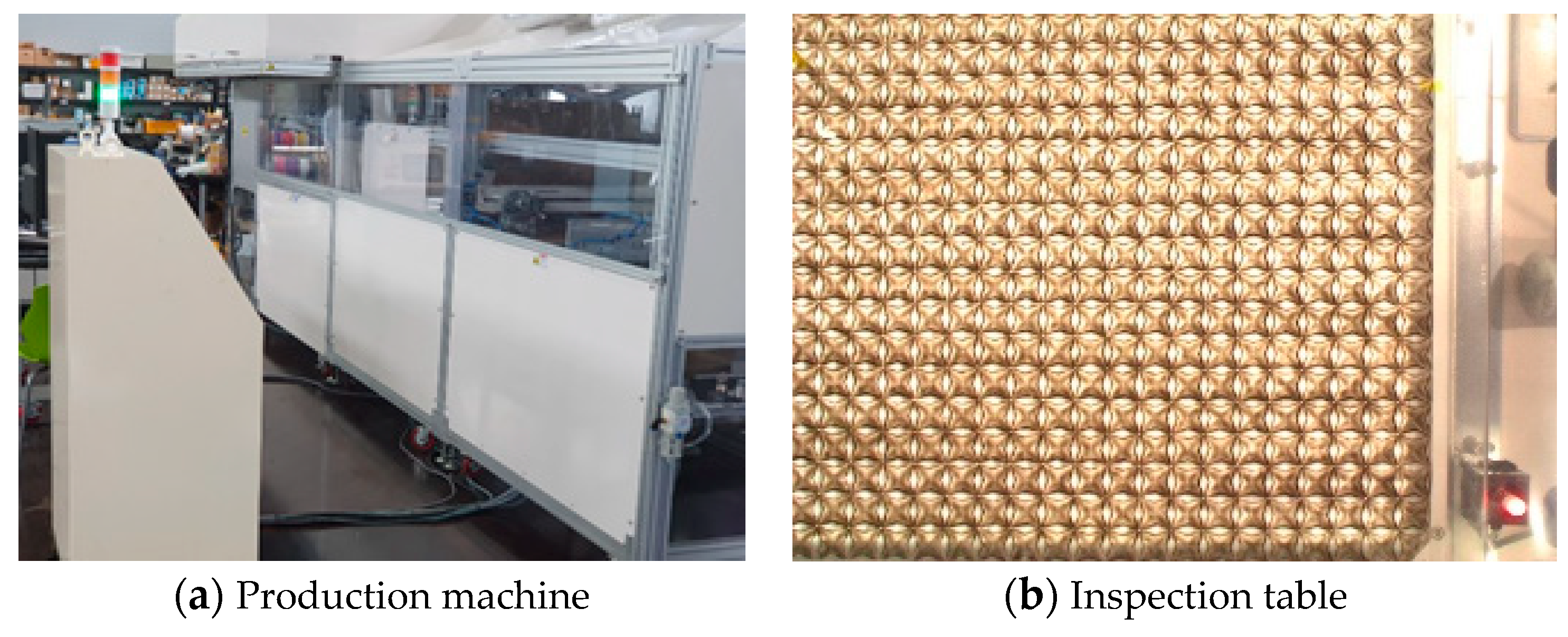
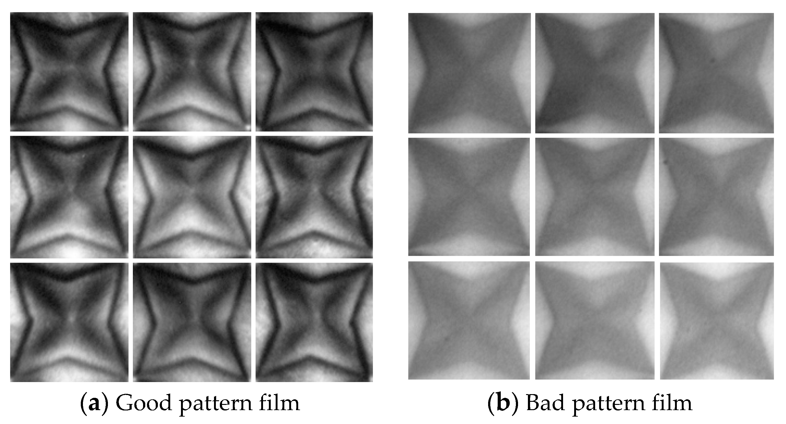
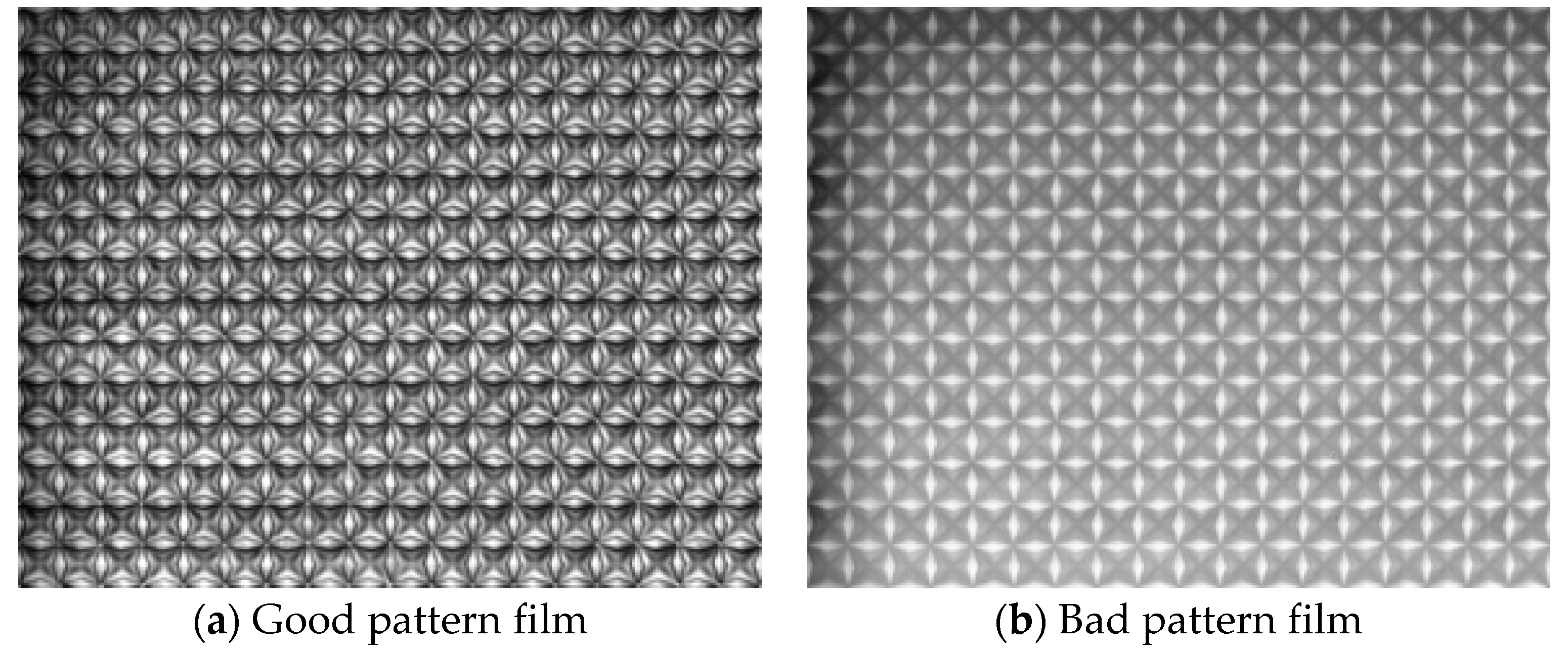
The 3D pattern film image is a three-dimensional image with a shadow formed on the opposite side of the incident surface of light, which cannot be confirmed by shape and touch but can only be confirmed by sight. Figure 1 shows 3D film images, of which (a) is a good 3D film image and (b) is a bad 3D film image. Figure 2a is a 3D film image printing, and (b) is an inspection machine. The 3D film image is printed in the printing machine, and after that, it is moved to the inspection machine and determined to be a good or bad 3D film image through the image taken with the camera. It is attached to the surface of various products such as cosmetics, liquor bottles, and book covers using good 3D film images classified through quality inspection.

Figure 1. Two types of 3D pattern film images.

Figure 2. Three-dimensional film image production and inspection machine.

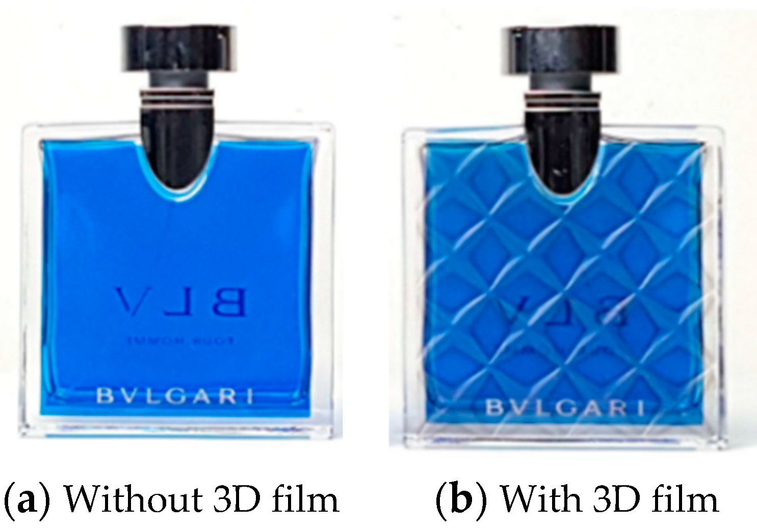
Figure 3a is a product without 3D film images, and (b) is a product with 3D film images. As shown in Figure 3, it can be used in marketing that stimulates the curiosity of buyers and increases their desire to purchase by attaching 3D film images to the surface of the product. However, the 3D film image is a recently developed technology that has not yet been commercialized, and is in the process of technical research for mass production and automatic quality inspection. In order to show the pattern of the 3D film image in three dimensions, the difference in contrast between pixels in the image should be large, and the contour of the pattern should be clear, as shown in Figure 1a. On the other hand, as shown in Figure 1b, if the difference in contrast between pixels in the image is not large and the contour of the pattern is not clear, it does not look three-dimensional. For this reason, quality inspection for 3D film images is essential. It is difficult to recognize the pattern in the 3D film image when the bad 3D film image is attached to the product. In addition, various methods for evaluating the quality of products produced using 3D printers, such as dimensional accuracy, surface roughness, and part density, have been extensively studied [1,2]. However, there are few methods used to classify good or bad 3D film images since it is a recently developed product. To inspect the 3D film pattern image, we can use various methods that have been used to detect and classify a particular pattern in an image, including image subtraction, binarization, segmentation, support vector machine (SVM), template matching, etc. [3,4,5,6,7,8,9,10,11,12,13,14,15,16,17,18,19,20,21,22,23,24,25,26]; however, it is not easy to classify good or bad 3D film images using the above-mentioned methods.

Figure 3. Commercial good without and with 3D film.

In this paper, we propose a method for classifying good or bad 3D film images based on a threshold using the width corresponding to a specific frequency of image histogram for a 3D film image. Since the method just uses the width of the specific height of the image histogram, the analysis process is simple. Additionally, it is not necessary to detect the pattern in an image because the method analyzes the characteristics of each pattern of good or bad 3D film images using the image histogram, and it can be classified even if the contrast of the pattern is low.

The composition of this paper is as follows. Section 2 introduces methods to detect a particular image in the image and classify good 3D film images and bad 3D film images. Section 3 describes the algorithm proposed in this paper, and Section 4 presents the experimental results of the proposed method. Finally, Section 5 concludes this paper.

2. Related Methods

In order to classify 3D film images as good or bad, a particular image or the characteristics of the images should be detected. Methods for detecting or classifying a particular object in an image include image subtraction, segmentation, SVM, and template matching. Image subtraction is used to extract a particular object in an image using differences between images or to find different parts between images, and studies using image subtraction have been recently published in the astronomical, astrophysical, and medical areas [3,4,5,6,7]. In particular, Hu et al. proposed the saccadic fast Fourier transform (SFFT) algorithm for image subtraction in time-domain astronomy, which uses a $\mathsf{\delta }$-function basis for kernel decomposition and performs the subtraction in Fourier space [4]. Fang et al. proposed an unsupervised approach using a cycle-GAN for efficient and accurate segmentation of pneumonia lesions in CT scans [5]. In this approach, they performed lung volume segmentation, healthy lung image synthesis, infected and healthy image subtraction, and binary lesion mask generation.

Binarization and edge detection are representative rule-based methods for segmentation. Binarization is a method of changing the pixel to black or white when it is high or low based on a certain threshold, and generally includes Global thresholding, adaptive thresholding, Otsu thresholding, etc. [8,9,10,11]. Adaptive thresholding is a method of applying different thresholds to each area, and Otsu thresholding is an algorithm that binarizes pixels in an image by finding thresholds that minimize variance or maximize differences between classes when classified into two classes. Recently, Fan et al. proposed an algorithm for road crack detection in images using deep learning and adaptive thresholding [10]. The algorithm extracted cracks from the road surface with an adaptive thresholding method, resulting in high accuracy in image classification and successful extraction of cracks. Hoang proposed an intelligent model based on image processing techniques for automatic crack recognition and analyses [11]. The model used the Otsu method for thresholding, followed by a gray intensity adjustment method called M2GLD, to improve the accuracy of crack detection results. Edge detection methods detect the edge of objects in an image by looking for a point where the brightness of the image changes suddenly through a differential equation, and they include Sobel edge detection, Canny edge detection, Laplacian edge detection, etc. [12,13,14]. Sobel edge detection is more resistant to noise than other edge detection algorithms and reacts more sensitively to diagonal edges than to vertical and horizontal components. Canny edge detection is an algorithm aimed at detecting strong edges that are not sensitive to noise. Unlike other edge detection algorithms, Laplacian edge detection uses a second-order differential equation. It is famous for edge detection because it detects the edges in a bright or dark area. Gong et al. have proposed an improvement to the traditional Canny edge operator for static gesture segmentation by using a combined filtering method and adaptive threshold algorithm, resulting in high accuracy in simple static gesture segmentation [15]. Bansal et al. have proposed an effective scheme for detecting blur in digital images based on edge analysis using the Laplacian operator, which can determine the extent of blur through the variance of the Laplacian method [16]. Additionally, the paper presents a simple and fast algorithm for estimating image noise using an easy edge detection algorithm and Laplacian operator, which performs well for different types of images over a large range of noise variances. Recently, edge detection research by Canny edge detection after applying HSV color in [17], and a geodesic active contour algorithm that often detects gradually developing boundaries in [18], have been published. Additionally, Morphological snakes, which are more stable and faster calculated through morphological operators performing expansion or erosion in [19], and morphological geodesic active contour algorithms by gently processing images with Gaussian filters after histogram equalization in image preprocessing as stated in [20], have been published.

SVM is an algorithm that classifies data based on the decision boundary. Recently, research on classifying good and bad images using an ensemble support vector machine in [21], a method of classifying the type of blur after classifying the bad image by blur extent estimation in [22], and the study of performing SVM after edge detection by applying Canny edge detection to images in [23], have been steadily published. In addition, Hemamalini et al. have discussed a method for assessing food quality using picture segmentation and machine learning [24]. After noise removal and histogram equalization, fruit photos were segmented using the K-means clustering technique and classified using machine learning algorithms such as KNN, SVM, and C4.5 to determine whether the fruits were damaged or not. Template matching methods for checking whether the template image matches the object in the image have been published in [25,26].

However, there are not many studies yet that have been used to classify 3D film images as good images and bad images, and there is a limit to solving the classification problem with the methods described above. This is because image subtraction only is insufficient for obtaining high accuracy; binarization should find the optimal threshold value. In addition, even though binarization thresholding methods are simple and easy to implement, binarization thresholding methods can be sensitive to noise, as the threshold value is often determined based on the intensity values of the pixels in the image. This can lead to the misclassification of pixels, resulting in an inaccurate representation of the image. Edge detection can provide information on the boundaries and shapes of objects within an image, which can be useful in tasks such as object recognition, tracking, and segmentation. In addition, edge detection algorithms are relatively fast and can be applied to large datasets. However, they can be sensitive to noise and may produce false positives or false negatives in noisy or low-contrast images. Moreover, the choice of algorithm and parameters can greatly affect the accuracy and quality of edge detection results and may require manual tuning. SVM has high accuracy in image classification tasks, particularly with complex datasets. However, SVM is not very fast and requires finding optimal hyper-parameters to determine the penalty for the error. On the other hand, the morphological geodesic active contour method can accurately segment complex objects with irregular shapes and boundaries. However, the algorithm can be computationally expensive, especially for large images or datasets. Moreover, it may not work well for images with overlapping objects or highly connected structures. Additionally, it is difficult to solve the classification problem using template matching because the 3D film image in this paper is not printed in the same texture and size. Furthermore, it is not easy to detect good and bad 3D film images in this paper because the contrasts of pixels in the image are different from one another.

3. Proposed Algorithm

Among the 3D film images, good 3D film images have a large contrast of pixels, and the contour is clear, but bad 3D film images do not have a large contrast between the pixels, and the contour is blurred. Therefore, in this paper, we propose a method to calculate the width of a specific height with an image histogram that can grasp the characteristics of the pattern in the image and check whether the 3D film image is bad based on the threshold value. To inspect the 3D film presented in Figure 1 of this paper, it is necessary to first crop each pattern image from the film. For this purpose, we used the fast Fourier transform algorithm. Therefore, in this section, we will first explain the method of extracting pattern images from the film through cropping, and then present the classification algorithm used for the quality inspection of 3D film images.

3.1. Cropping Pattern Images on Film Using Fast Fourier Transform Algorithm

To inspect the pattern in the 3D film of Figure 1, the image must be cut for each pattern. We use the fast Fourier transform to cut the image by pattern in the printed 3D film [27]. Let $I\left(x,y\right)$ be $N\times N$ binarized image in the spatial domain, which is sampled from the discrete Fourier transform and is defined as $F\left(n,m\right)$ as shown in Equation (1).

$$F\left(n,m\right)={{\displaystyle -}}_{x=0}^{N-1}{{\displaystyle -}}_{y=0}^{N-1}I\left(x,y\right)e^{-2\pi i\left(\frac{xn}{N}+\frac{ym}{N}\right)},$$

(1)

where the exponential term is a fundamental function representing sine waves and cosine waves with increasing frequencies corresponding to each $F\left(n,m\right)$ in Fourier space. For the Fourier image $F\left(n,m\right)$, we convert it to spatial domain $I\left(x,y\right)$, as shown in Equation (2).

$$I\left(k,l\right)=\frac{1}{N^2}{{\displaystyle -}}_{n=0}^{N-1}{{\displaystyle -}}_{m=0}^{N-1}F\left(n,m\right)e^{2\pi i\left(\frac{kn}{N}+\frac{lm}{N}\right)},$$

(2)

Because the Fourier transform is separable, it can be decomposed into two equations. Equation (3) represents the first transformation of the spatial image to an intermediate image using N one-dimensional Fourier transformations. Equation (4) represents the transformation of the intermediate image to the final image in a series of 2N one-dimensional transformations.

$$F\left(n,m\right)=\frac{1}{N}{{\displaystyle -}}_{l=0}^{N-1}T\left(n,l\right)e^{-2\pi i\left(\frac{ml}{N}\right)},$$

(3)

$$T\left(n,l\right)=\frac{1}{N}{{\displaystyle -}}_{k=0}^{N-1}T\left(k,l\right)e^{-2\pi i\left(\frac{kn}{N}\right)},$$

(4)

From Equation (4), we use the real part of the processed image because the imaginary part is almost always negligible, and images are real-valued functions. We determine the index of the white pixel values of $I\left(k,l\right)$ to obtain the horizontal $I_i\left(i,j\right)$ and vertical $I_j\left(i,j\right)$, as shown in Equations (5) and (6).

$$I_i\left(i,j\right)=\left\{\begin{array}{c}255, T\left(n,l\right)>0\\ 0, elsewhere\end{array}\right.,$$

(5)

$$I_j\left(i,j\right)=\left\{\begin{array}{c}255, T\left(n,l\right)>0\\ 0, elsewhere\end{array}\right.,$$

(6)

From the result in Equations (5) and (6), the pixel coordinates are obtained by the intersection. After that, the intersection information can be used to cut the pattern images of the 3D film.

3.2. Classification Using an Optimal width of Image Histogram

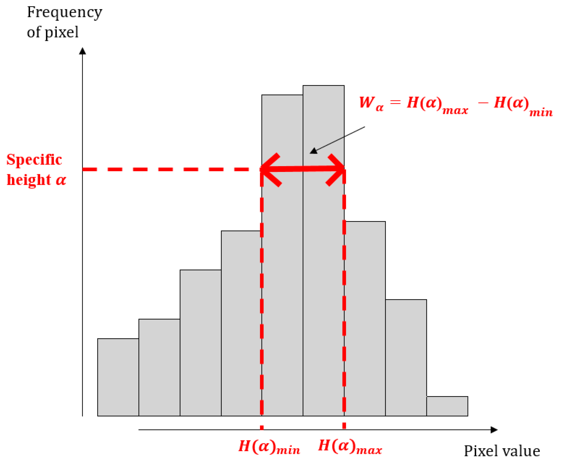
Using the fast Fourier transform algorithm mentioned earlier, we classify 3D film pattern images into good or bad by cutting them into patterns. The algorithm for determining the quality of the pattern image is as follows. First, convert the image to a gray image, and then obtain the image histogram of the gray image. Then, determine the specific height of the image histogram $\alpha$, and find the maximum pixel value and the minimum pixel value corresponding to $\alpha$, and then obtain the width of the corresponding height $\alpha$. The equation for calculating the width of the image histogram $W\left(\alpha \right)$ is as follows:

$$W\left(\alpha \right)=H{\left(\alpha \right)}_{max}-H{\left(\alpha \right)}_{min},$$

(7)

where $H{\left(\alpha \right)}_{max}$ and $H{\left(\alpha \right)}_{min}$ are the maximum value and the minimum value for a specific height $\alpha$ of the image histogram, respectively. $W\left(\alpha \right)$ represents the width of the pixel, which is the difference between $H{\left(\alpha \right)}_{max}$ and $H{\left(\alpha \right)}_{min}$. Figure 4 shows the process of obtaining width $W\left(\alpha \right)$. After calculating the width $W\left(\alpha \right)$, the 3D film image is classified as a good 3D film image or a bad 3D film image based on the predetermined threshold $\beta$. The decision can be defined as follows:

$$R=\left\{\begin{array}{c}1, W\left(\alpha \right)>\beta \\ 0, otherwise\end{array}\right.,$$

(8)

where $R$ is the class label of the image. When $R$ = 1, it is a good image, and when $R$ = 0, it is a bad image. The procedure of the proposed algorithm is shown in Figure 5.

Figure 4. The $H{\left(\mathsf{\alpha }\right)}_{min}$ and $H{\left(\alpha \right)}_{max}$ at specific height $\mathsf{\alpha }$ in the image histogram.

Figure 5. Procedures of the proposed algorithm.

4. Experimental Results and Discussion

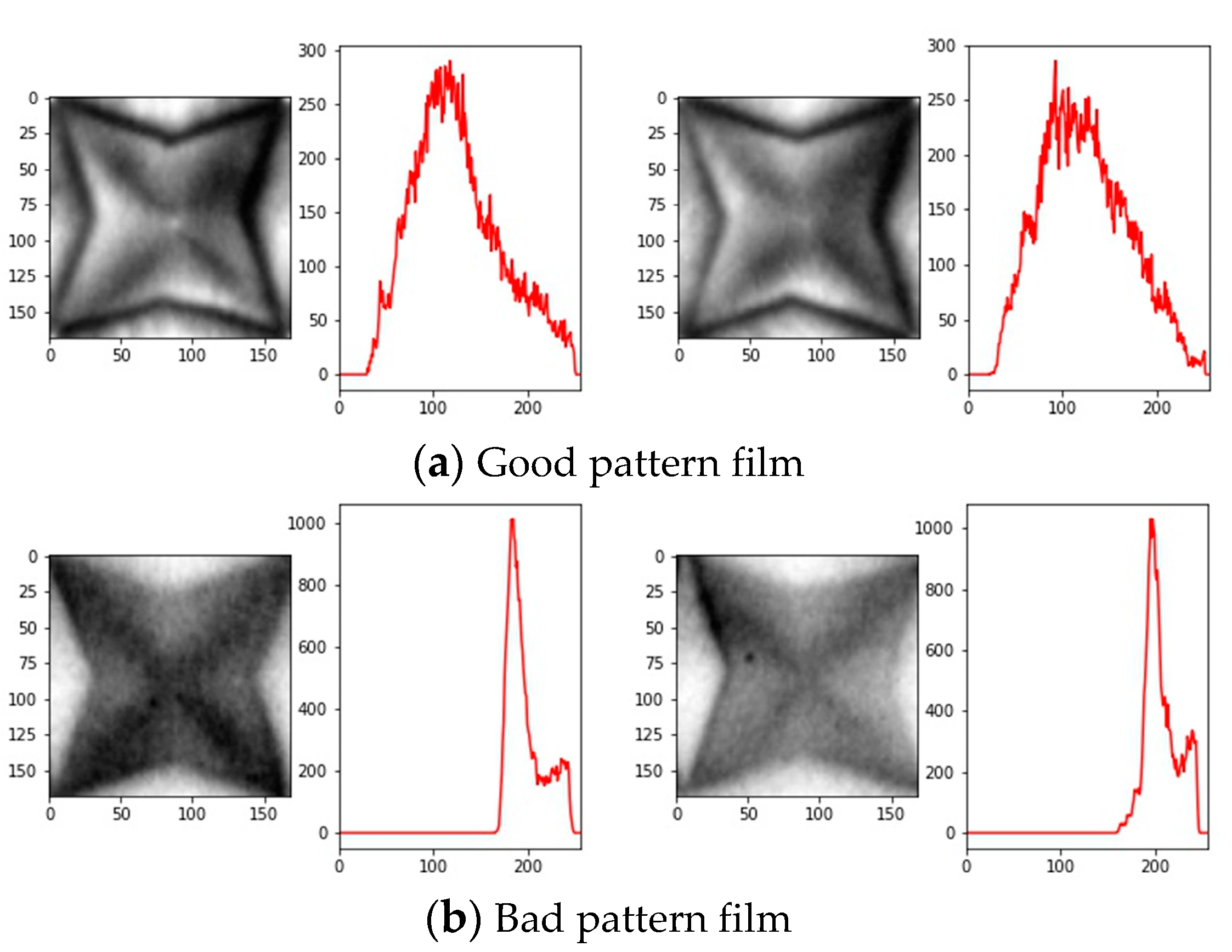
In order to evaluate the performance of the proposed algorithm, the experiment was conducted using a total of 2580 3D film images, of which 2136 are good 3D pattern film images, and 714 are bad 3D pattern film images. The evaluation was performed by cropping all patterns individually into a size of 169 × 169, as shown in Figure 6. The experiments of this work were performed on Windows 10 Pro and Python 3.6. Figure 7a shows an image histogram for good 3D film images, and (b) shows an image histogram for bad 3D film images. As shown in Figure 7a, the width of the pixel value on the x-axis is wide because the contrast of the pixel in the image was high, but (b) shows that the width of the pixel is narrow because the contrast of the pixel in the image was low. Based on these characteristics of good and bad 3D film images, the results of obtaining the width of the height from 1/10 to 9/10 for the image histogram for each image are shown in Table 1. As shown in Table 1, when comparing the minimum value and the maximum value of the width of good and bad 3D film images, it can be observed that the lower the height of the image histogram, the larger the difference in width between good and bad 3D film images. As a result of determining the threshold for each height of the image histogram, the classification accuracy was found to be over 99% from 1/10 to 5/10 of the image histogram height, and in particular, the classification accuracy was the highest at 99.34% at 3/10 of the image histogram height.

Figure 6. Separated good and bad 3D film images.

Figure 7. Good and bad 3D film images with image histogram.

Table 1. Classification accuracy according to the height of the image histogram.

	Specific Height	1/10	2/10	3/10	4/10	5/10	6/10	7/10	8/10	9/10
Good Pattern	Min	85	63	29	23	20	12	9	2	1
	Max	241	240	229	195	190	158	128	99	89
Bad Pattern	Min	43	22	17	12	9	6	5	3	1
	Max	133	106	86	70	66	58	55	53	40
Threshold		120	95	65	55	35	30	20	15	5
Accuracy (%)		99.23	99.27	99.34	99.13	99.09	98.78	97.55	73.42	82.40

To evaluate the performance of the proposed algorithm, the analysis results were compared using image subtraction, Canny edge detection, Canny edge detection with HSV [10], Otsu thresholding, morphological geodesic active contour [13], and SVM with Canny edge detection [16]. Figure 8a–l show good and bad 3D film images originally and with image subtraction, Canny edge detection, Canny edge with HSV, Otsu thresholding, and morphological geodesic active contour, respectively. Figure 8b shows the result of applying the image subtraction of the control good 3D film image to good 3D film images, and (h) shows the image subtraction image of the control good 3D film image and bad 3D film images, where black is the difference between the two images. In Canny edge detection, the minimum threshold value and the maximum threshold value were set to 10 and 50, respectively. As shown in Figure 8c,d, a lot of edges in the image were detected when Canny edge detection was applied. On the other hand, Figure 8i,j show that the pattern of the image was hardly detected when Canny edge detection was applied; (k) and (l) show that the pattern was not accurately detected. Therefore, it was found that most of the pattern detection results in the bad 3D film image were almost poor. We used the Edge Preservation Index (EPI) [28] to evaluate the performance of the comparison methods. This metric is used to measure the preservation of image edges before and after processing. The equation is as follows

$$\mathrm{EPI}=\frac{{\displaystyle \sum }\left|P_s\right(i,j)-P_s(i-1,j+1\left)\right|}{{\displaystyle \sum }\left|P_{ij}\right(i,j)-P_{ij}(i-1,j+1\left)\right|},$$

(9)

where P_s is the value of the image-processed image pixel in (i, j), P_ij is the value of the original image pixel in (i, j); the P_s(i, j) and P₀(i, j) are in the edge area where intensity sharply varies. From the EPI results, a s higher EPI value indicates that the processed image preserves the edges of the original image. On the contrary, a lower EPI value means that the processed image significantly alters or removes the edges of the original image, resulting in a lower degree of preservation. Table 2 shows the results of comparison methods of the EPI for good pattern film images and bad pattern film images of Figure 8. In Table 2, all methods except for image subtraction produced values over 1 for the good pattern images, with morphological geodesic active contour showing the highest value.

Figure 8. Good and bad 3D film images with comparison algorithms.

Table 2. Results of Edge Projection Index for Good pattern film images and Bad pattern film images.

Algorithm	Good Pattern Film Images				Bad Pattern Film Images
	Img1	Img2	Img3	Img4	Img1	Img2	Img3	Img4
Image subtraction	0.5445	0.4736	0.5171	0.5040	0.2477	0.2735	0.2372	0.2694
Canny edge detection	3.9533	3.9257	4.6248	3.9869	2.0604	2.1220	1.9288	2.0198
Canny edge detection with HSV [17]	3.6100	3.5531	3.8108	3.6666	1.8198	2.0888	1.8439	1.9961
Otsu thresholding	4.3954	4.3134	4.6248	4.4331	2.0672	2.1133	1.9076	1.9919
Morphological geodesic active contour [20]	13.4196	13.1801	14.1203	13.5010	6.2879	6.4296	5.8185	6.0841

This indicates that image subtraction does not properly detect the edges of the image, and that morphological geodesic active contour detects edges the best. In addition, Canny edge detection and Canny edge detection with HSV produced relatively small values compared to Otsu thresholding, indicating that they detected too many edges. For the bad pattern images, all methods except for image subtraction produced values over 1, with morphological geodesic active contour showing the highest value. On the other hand, Canny edge detection, Canny edge detection with HSV, and Otsu thresholding produced similar values. However, as seen in the results of Figure 8i–k, the methods failed to detect the bad pattern images properly, but all EPI values were over 1. This is because the original images also had very blurry contours, making it difficult to detect the edges.

The structural similarity index (SSIM) [29] was used to evaluate the similarity between the two images. SSIM is a measure that evaluates similarity using brightness, contrast, and structure of information of two images. The equation for comparing the structure of the pixels constituting the image is as follows:

$$\begin{gathered} SSIM\left(x,y\right)=B\left(x,y\right)·C\left(x,y\right)·R\left(x,y\right) \\ =\frac{4{\mu }_x{\mu }_y{\sigma }_{xy}}{\left({\mu }_x^2+{\mu }_y^2\right)\left({\sigma }_x^2+{\sigma }_y^2\right)} , \\ \mathrm{where} B\left(x,y\right)=\frac{2{\mu }_x{\mu }_y}{{\mu }_x^2+{\mu }_y^2},\hspace{1em}\hspace{1em}C\left(x,y\right)=\frac{2{\sigma }_x{\sigma }_y}{{\sigma }_x^2+{\sigma }_y^2}, \\ R\left(x,y\right)=\frac{2{\sigma }_{xy}}{{\sigma }_x{\sigma }_y} \end{gathered}$$

(10)

where $B\left(x,y\right)$, $C\left(x,y\right)$, and $R\left(x,y\right)$ represent the average brightness, contrast, and correlation of the two images, respectively. ${\mu }_x,$ ${\mu }_y$, ${\sigma }_x^2$, ${\sigma }_y^2$ and ${\sigma }_{xy}$ are the mean brightness of the original image, mean brightness of image processed image, global variance in the original image, global variance in image processed image, and covariance between the original and image processed images, respectively. From the SSIM results, if the value is greater than the threshold (0.5), it was classified as similar images, and if the value is small, the images are not similar. When performing SSIM, we used the first image of the good image in Figure 7a as the reference image. Table 3 shows the classification results of good and bad 3D film images for each conventional method.

Table 3. Classification accuracy and computation time of the proposed and comparison algorithms.

Algorithm	Accuracy (%)	Computation Time (sec)
Proposed algorithm	99.34	3240.225
Image subtraction	76.75	12.126
Canny edge detection	22.62	12.158
Canny edge detection with HSV [17]	25.05	54.869
Otsu thresholding	39.28	8.135
Morphological geodesic active contour [20]	72.07	2074.59
SVM with Canny edge detection [23]	76.58	21.314

From Table 3, the computational time was the longest for morphological geodesic active contour and the proposed method, but the rest of the algorithms were faster than the aforementioned, within 1 min. However, the accuracy of the proposed algorithm was 99.34% when the image histogram’s specific height $\mathsf{\alpha }$ was 3/10, and there was a large difference in accuracy from other methods. In particular, Canny edge detection, Canny edge detection with HSV, and Otsu thresholding could hardly classify good and bad 3D film images. This is because the contrast of pixels in a bad 3D film image is low.

5. Conclusions

In 3D film image, it is not easy to inspect whether the 3D film image is good or bad because in 3D film images, the pattern contour is not clear, and the contrast of pixels in the image is low. In addition, there are few methods used to classify good or bad 3D film images since they are a recently developed product. In this paper, we proposed a quality inspection method that classifies good and bad 3D film images based on a threshold value by calculating the width for a specific height of the image histogram that shows the characteristics of the image. Through the experiment, it was shown that the classification accuracy of the proposed algorithm was the highest, at 99.34%, at 3/10 of the height of the image histogram. The proposed quality inspection method took a little bit longer than other algorithms, but the algorithm was simple, and the test accuracy was much higher than other algorithms. Additionally, it was shown that there was no need to detect patterns in the image, and quality inspection was possible even if the contrast of the image was low. In future work, we plan to study methods for automatic quality inspection of 3D film images.

References

1. Yang, Y.; Chen, Y.; Wei, Y.; Li, Y. 3D Printing of shape memory polymer for functional part fabrication. Int. J. Adv. Manuf. Technol. 2015, 84, 2079–2095. [Google Scholar] [CrossRef]
2. Ugur, M.D.; Gharehpapagh, B.; Yaman, U.; Dolen, M. The role of additive manufacturing in the era of Industry 4.0. Procedia Manuf. 2017, 11, 545–554. [Google Scholar]
3. Colman, I.L.; Bedding, T.R.; Huber, D.; Kjeldsen, H. The kepler IRIS catalog: Image subtraction light curves for 9150 stars in and around the open clusters NGC 6791 and NGC 6819. Astrophys. J. Suppl. Ser. 2022, 258, 39–53. [Google Scholar] [CrossRef]
4. Hu, L.; Wang, L.; Chen, X.; Yang, J. Image Subtraction in Fourier Space. Astrophys. J. 2022, 936, 157. [Google Scholar] [CrossRef]
5. Fang, C.; Liu, Y.; Liu, Y.; Liu, M.; Qiu, X.; Li, Y.; Wen, J.; Yang, Y. Label-free coronavirus disease 2019 lesion segmentation based on synthetic healthy lung image subtraction. Med. Phys. 2022, 49, 4632–4641. [Google Scholar] [CrossRef]
6. Cao, Y.; Nugent, P.E.; Kasliwal, M.M. Intermediate palomar transient factory: Realtime image subtraction pipeline. Publ. Astron. Soc. Pac. 2016, 128, 114502. [Google Scholar] [CrossRef]
7. Masci, F.J.; Laher, R.R.; Rebbapragada, U.D.; Doran, G.B.; Miller, A.A.; Bellm, E.; Kasliwal, M.; Ofek, E.O.; Surace, J.; Shupe, D.L.; et al. The IPAC image subtraction and discovery pipeline for the Intermediate Palomar Transient Factory. Publ. Astron. Soc. Pac. 2016, 129, 014002. [Google Scholar] [CrossRef]
8. Mustafa, W.A.; Kader, M.A. Binarization of document images: A comprehensive review. In Proceedings of the International Conference on Green and Sustainable Computing (ICoGeS), Kuching, Malaysia, 25–27 November 2017; p. 012023. [Google Scholar]
9. Tensmeyer, C.; Martinez, T. Historical document image binarization: A review. SN Comput. Sci. 2020, 1, 173. [Google Scholar] [CrossRef]
10. Fan, R.; Bocus, M.J.; Zhu, Y.; Jiao, J.; Wang, L.; Ma, F.; Cheng, S.; Liu, M. Road crack detection using deep convolutional neural network and adaptive thresholding. In Proceedings of the 2019 IEEE Intelligent Vehicles Symposium (IV), Paris, France, 9–12 June 2019; pp. 474–479. [Google Scholar]
11. Hoang, N.D. Detection of surface crack in building structures using image processing technique with an improved Otsu method for image thresholding. Adv. Civ. Eng. 2018, 2018, 3924120. [Google Scholar] [CrossRef]
12. Owotogbe, Y.S.; Ibiyemi, T.S.; Adu, B.A. Edge detection techniques on digital images-a review. Int. J. Innov. Sci. Res. Technol. 2019, 4, 329–332. [Google Scholar]
13. Jing, J.; Liu, S.; Wang, G.; Zhang, W.; Sun, C. Recent advances on image edge detection: A comprehensive review. Neurocomputing 2022, 503, 259–271. [Google Scholar] [CrossRef]
14. Lorencin, I.; Anđelić, N.; Španjol, J.; Car, Z. Using multi-layer perceptron with Laplacian edge detector for bladder cancer diagnosis. Artif. Intell. Med. 2020, 102, 101746. [Google Scholar] [CrossRef] [PubMed]
15. Gong, S.; Li, G.; Zhang, Y.; Li, C.; Yu, L. Application of static gesture segmentation based on an improved canny operator. J. Eng. 2019, 2019, 543–546. [Google Scholar] [CrossRef]
16. Bansal, R.; Raj, G.; Choudhury, T. Blur image detection using Laplacian operator and Open-CV. In Proceedings of the 2016 International Conference System Modeling & Advancement in Research Trends (SMART), Moradabad, India, 25–27 November 2016; pp. 63–67. [Google Scholar]
17. Septiarini, A.; Hamdani, H.; Sari, S.U.; Hatta, H.R.; Puspitasari, N.; Hadikurniawati, W. Image processing techniques for tomato segmentation applying k-means clustering and edge detection approach. In Proceedings of the International Seminar on Machine Learning, Optimization, and Data Science, jakarta, Indonesia, 29–30 January 2021; pp. 92–96. [Google Scholar]
18. Ma, J.; Wang, D.; Wang, X.P.; Yang, X. A fast algorithm for geodesic active contours with applications to medical image segmentation. arXiv 2020, arXiv:2007.00525v1. [Google Scholar]
19. Álvarez, L.; Baumela, L.; Neila, P.M.; Henríquez, P. A real time morphological snakes algorithm. Image Process. Online 2014, 2, 1–7. [Google Scholar] [CrossRef]
20. Mlyahilu, J.N.; Mlyahilu, J.N.; Lee, J.E.; Kim, Y.B.; Kim, J.N. Morphological geodesic active contour algorithm for the segmentation of the histogram-equalized welding bead image edges. IET Image Process. 2022, 16, 2680–2696. [Google Scholar] [CrossRef]
21. Wang, R.; Li, W.; Li, R.; Zhang, L. Automatic blur type classification via ensemble SVM. Signal Process. Image Commun. 2019, 71, 24–35. [Google Scholar] [CrossRef]
22. Hsu, P.; Chen, B.Y. Blurred image detection and classification. In Proceedings of the International Conference on Multimedia Modeling, Kyoto, Japan, 9–11 January 2008; pp. 277–286. [Google Scholar]
23. Salman, A.; Semwal, A.; Bhatt, U.; Thakkar, V.M. Leaf classification and identification using canny edge detector and SVM classifier. In Proceedings of the International Conference on Inventive Systems and Control, Coimbatore, India, 19–20 January 2017; pp. 1–4. [Google Scholar]
24. Hemamalini, V.; Rajarajeswari, S.; Nachiyappan, S.; Sambath, M.; Devi, T.; Singh, B.K.; Raghuvanshi, A. Food quality inspection and grading using efficient image segmentation and machine learning-based system. J. Food Qual. 2022, 2022, 1–6. [Google Scholar] [CrossRef]
25. Thomas, M.V.; Kanagasabapthi, C.; Yellampalli, S.S. VHDL implementation of pattern based template matching in satellite images. In Proceedings of the International Conference on Smart Technologies for Smart Nation, Bengaluru, India, 17–19 August 2017; pp. 820–824. [Google Scholar]
26. Satish, B.; Jayakrishnan, P. Hardware implementation of template matching algorithm and its performance evaluation. In Proceedings of the International Conferences on Microelectronic Devices and Technologies, Vellore, India, 10–12 August 2017; pp. 1–7. [Google Scholar]
27. Mlyahilu, J.; Kim, J. A Fast Fourier Transform with Brute Force Algorithm for Detection and Localization of White Points on 3D Film Pattern Images. J. Imaging Sci Technol. 2021, 66, 030506. [Google Scholar] [CrossRef]
28. Joseph, J.; Jayaraman, S.; Periyasamy, R.; Renuka, S.V. An edge preservation index for evaluating nonlinear spatial restoration in MR images. Curr. Med. Imaging Rev. 2017, 13, 58–65. [Google Scholar] [CrossRef]
29. Sara, U.; Morium, A.; Uddin, M.S. Image quality assessment through FSIM, SSIM, MSE and PSNR—A comparative study. J. Comput. Commun. 2019, 7, 8–18. [Google Scholar] [CrossRef]
Disclaimer/Publisher’s Note: The statements, opinions and data contained in all publications are solely those of the individual author(s) and contributor(s) and not of MDPI and/or the editor(s). MDPI and/or the editor(s) disclaim responsibility for any injury to people or property resulting from any ideas, methods, instructions or products referred to in the content.
Article Metrics
Citations
Article Access Statistics
Multiple requests from the same IP address are counted as one view.