1. Introduction
The pointing performance of a spacecraft is continuously advancing due to the quick developments in space technology. For example, the Earth observation spacecraft [
1]. The Seasat/Landsat-1, in the 1970s, had a pointing accuracy of 1°–0.3° and an attitude stability of 5 × 10
−2°/s–1 × 10
−2°/s. The SPOT/Landsat-2 satellites, in the 1980s, had a pointing accuracy of 0.3°–0.03° and an attitude stability of 3 × 10
−3°/s–3 × 10
−5°/s. The ADEOS satellite, in the 1990s, had a pointing accuracy of 0.3°–0.02° and an attitude stability of 1 × 10
−3°/s–1 × 10
−6°/s. The pointing accuracy of the Hilios/IRS-P satellites in the new century was 0.1–0.001°, and the attitude stability was better than 1 × 10
−4°/s. The same trend holds true for space telescopes and interferometers [
2]. The Infrared Astronomical Satellite (IRAS) had an absolute pointing accuracy of 30 arcseconds with a pointing stability of 10 arcseconds. The Hubble Space Telescope launched on 24 April 1990, had a radial pointing stability of 0.007 arcseconds RMS over periods between 60 s and 24 h. The Infrared Space Observatory (ISO), launched on 17 November 1995, was required to achieve 11.7 arcseconds radial absolute accuracy at 2-sigma, 2.7 arcseconds half-cone stability at 2-sigma over a time period of 30 s and 2.8 arcseconds half-cone drift at 2-sigma per hour. The James Webb Space Telescope (JWST), launched on 25 December 2021, had a line-of-sight (LOS) stability that was better than 0.005 arcseconds RMS, a change in mean pointing over a timescale of a few seconds less than 0.0035 arcseconds, and a roll stability below 0.0035 arcseconds.
To satisfy such strict requirements, a wide range of perturbation causes must be carefully taken into account. Eyerman [
3] provided a thorough overview of the different disturbance sources, including both internal and external disturbance sources, which caused spacecraft’ platforms to vibrate in 1990. The external disturbance sources mainly come from the spacecraft’s external space environment and include torques produced from gravity gradients, atmospheric drag, radiation pressure, magnetic dipoles, particle impacts, and eclipse transients. The external disturbance sources mainly induce the low-frequency vibration of the large flexible accessory of the spacecraft platform (<1 Hz). This kind of vibration can generally be eliminated by compensation of attitude and orbit control systems (AOCS) [
4] or structural vibration control of flexible attachments [
5,
6]. Internal disturbance sources mainly come from various moving parts inside the spacecraft, such as reaction wheel assembly (RWA), control moment gyros (CMGs), cryocoolers, solar wing driving mechanisms, antenna driving mechanisms, etc. [
7]. These moving components and systems typically have non-ideal characteristics, such as residual unbalance in the rotor of the RWA, unstable output in the solar wing drive motor, etc., which cause additional disturbance while in operation. This trait is intrinsic to the moving parts on the spacecraft because these disturbance factors are essentially unavoidable. The vibration caused by the moving parts inside the spacecraft is specifically referred to as microvibrations. Although the onboard microvibration has a very small amplitude, it is one of the major factors contributing to platform jitter and a decline in pointing stability and precision. The frequency range of a microvibration is very wide (1 Hz–1000 Hz), among which the most prominent disturbance is in the range of 10–200 Hz. It goes far beyond AOCS’s range. To prevent its impact on the spacecraft, it is essential to research and implement practical countermeasures.
One of the most significant sources of disturbance, RWA has drawn the attention of many academics. Examples include the empirical and analytical models of RWA disturbances, in references [
8,
9,
10], parameter estimation, identification of RWA, in references [
11,
12], and nonlinear electromechanical coupling dynamics of RWA, in reference [
13]. Evaluating the influence of the disturbance on the pointing accuracy of a spacecraft is an arduous task because it involves multiple disciplines, such as structural dynamics, control systems, mechanisms, and system engineering [
14]. The integrated modeling is an efficient method, as demonstrated by the development of DOCS (Dynamics–Optics–Controls–Structures) by SSL (Space System Laboratory, Cambridge, MA, USA) at MIT [
15,
16], IMOS (Integrated Modeling of Optical Systems) by Jet Propulsion Laboratory (JPL) (Pasadena, CA, USA) [
17], Integrated Modeling Environment (IME) by Goddard Space Flight Center (Greenbelt, MD, USA), Constellation Software Engineering (CSE) (Annapolis, MD, USA) [
18], and Integrated Framework by Korea Advanced Institute of Science and Technology (Daejeon, Republic of Korea) [
19].
Acquisition of the frequency response function (FRF) from the disturbance source to the sensitive payload is one of the most crucial stages in integrated modeling, and many scholars have worked hard on this [
20,
21,
22]. It is challenging to measure the FRF directly due to the restricted room for RWA installation in real spacecraft, particularly in small satellites. The standard procedure is to use a shaker to measure the FRF from the location of the RWA installation to the sensitive payload. The response of the sensitive payload derived by multiplying the FRF and the disturbance force and tongue measured in a hard-mounted boundary condition is quite different from the test result because of the coupling between the RWA and the support structure. Therefore, additional complex tests are needed to compensate for the disturbance force of the RWA, such as the static dynamic mass measurement techniques, for when the RWA is at 0 rpm [
23,
24], the dynamic mass measurement method, which includes the gyroscopic effects in its accelerants [
25,
26], a combination of the experiments in a static condition, and analysis that includes the gyroscopic effect through the RWA finite element (FE) model [
27].
There are many various FRF estimation techniques [
28,
29,
30], yet the most widely used ones are the
H1,
H2, and
Hv algorithms. The
H1 method assumes that there is no error in the references, while the
H2 method assumes that there is no error in the responses. The
Hv method provides the most precise estimate by accounting for the input and output noises. This paper presents a general approach based on the
Hv algorithm to acquire the FRF from the disturbance source to the sensitive payload, which is excited by the RWA, itself, and does not need any additional excitation source. The FRF obtained by this method accounts for the coupling between the RWA and the spacecraft, so the response of the sensitive load can be obtained by multiplying the RWA disturbance measured at a fixed interface using the FRF.
The paper is organized as follows: in
Section 2, an integrated model of a high-precision optical remote sensing satellite is developed that consists of the disturbance model, structural dynamic model, and the optical model. In
Section 3, a general method to obtain the FRF from the disturbance source to the sensitive payload is proposed. In
Section 4, we evaluate the microvibration of the entire satellite using different RWAs as the excitation source. Finally, conclusions are drawn in
Section 5.
2. Integrated Modeling
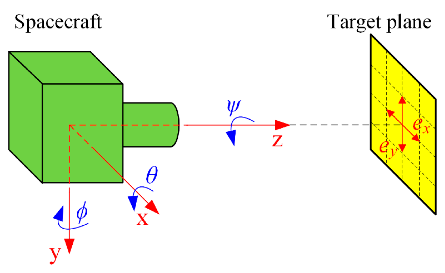
Considering a pointing scene, the pointing error is described as the difference between the actual orientation and the desired orientation of the spacecraft’s LOS with respect to the target plane [
31], as shown in
Figure 1. It is described by two translations (
ex,
ey) and one rotation (
ψ) on the target plane or by three rotations (
θ,
ϕ,
ψ) about the body axes of the pointing system.
The disturbance force and torque of the RWA can result in the image motion of the sensitive optical payload. The image motion is decomposed into a sum of displacement, smear, and jitter [
32,
33]. The image motion
p(
t) can be modeled by:
In this paper, we take an optical remote-sensing satellite as the research object. The payload of the satellite is a high-resolution optical remote sensing camera with a resolution greater than 1.1 m. The satellite is in a 535 km sun-synchronous orbit and weighs 65 kg. Three RWAs were used by the satellite to change its attitude.
Figure 2 depicts a 3D model of the satellite, and
Table 1 lists its parameters.
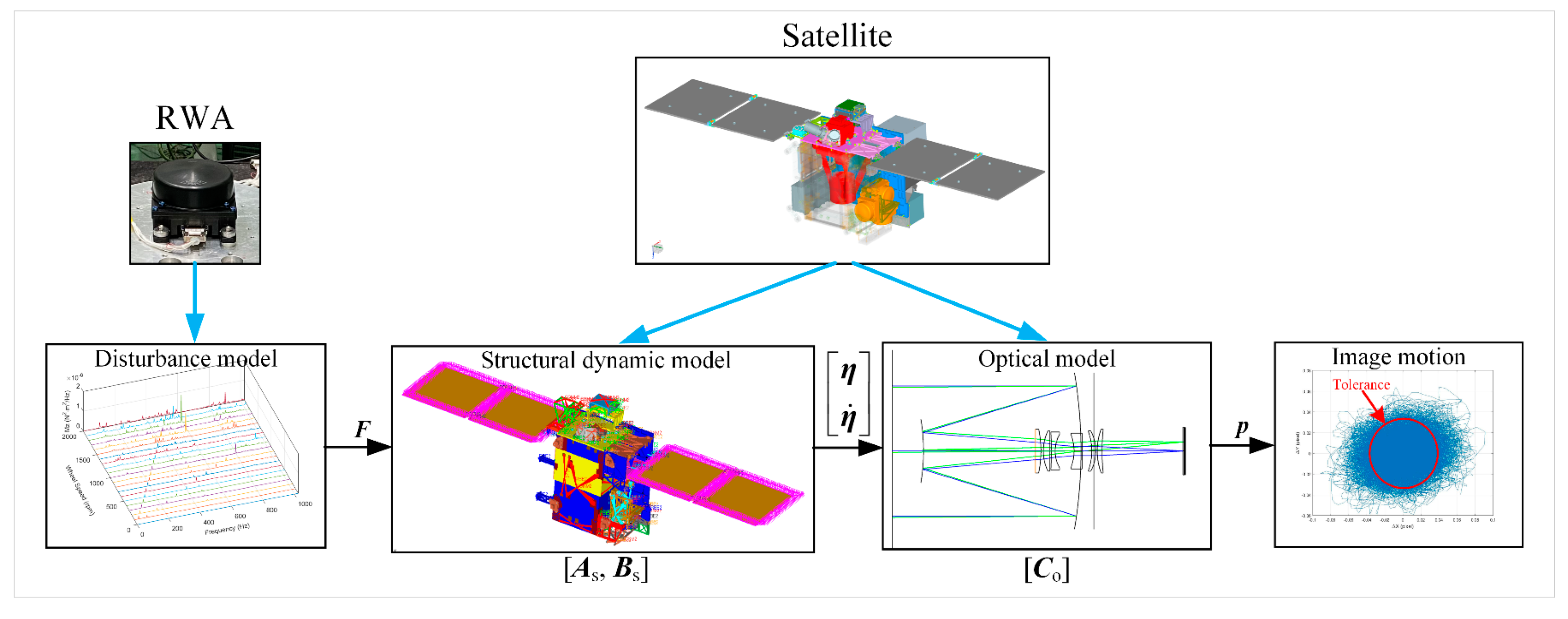
The integrated model of the satellite consists of three parts, ignoring the effect of AOCS: disturbance model, structural dynamic model, and optical model. The three parts are connected to each other through input and output interfaces. The output of the disturbance model is
F, which acts on the structural dynamic model of the satellite and causes the camera’s optics to shift slightly. This displacement
η is used as the input of the optical model to obtain the final image motion
p. The block diagram of the integrated model is shown in
Figure 3.
2.1. Disturbance Model
RWA is the primary disturbance source in most spacecrafts and the disturbance model of the RWA has been studied for several decades. There are currently three different types of disruption disturbance models. They are the empirical model [
34], the analytic model [
8,
9], and the semi-analytic model [
35]. This paper does not place a strong focus on the disturbance model, and in order to derive the integrated model, we use the empirical model.
The disturbance of the RWA is modeled as a series of discrete harmonics with amplitudes proportional to the square of the wheel speed and frequencies that change linearly with wheel speed [
9]:
where,
Fj(
t) is the
jth component of
F,
F = [
Fx,
Fy,
Fz,
Mx,
My,
Mz]
T.
n is the number of harmonics included in the model,
Ci is the amplitude coefficient of the
ith harmonic, Ω is the wheel speed,
hi =
ωi/Ω is the
ith harmonic number, equal to the ratio of the frequency
ωi to the wheel speed Ω, and
αi is a random phase (assumed to be uniform over (0, 2π)).
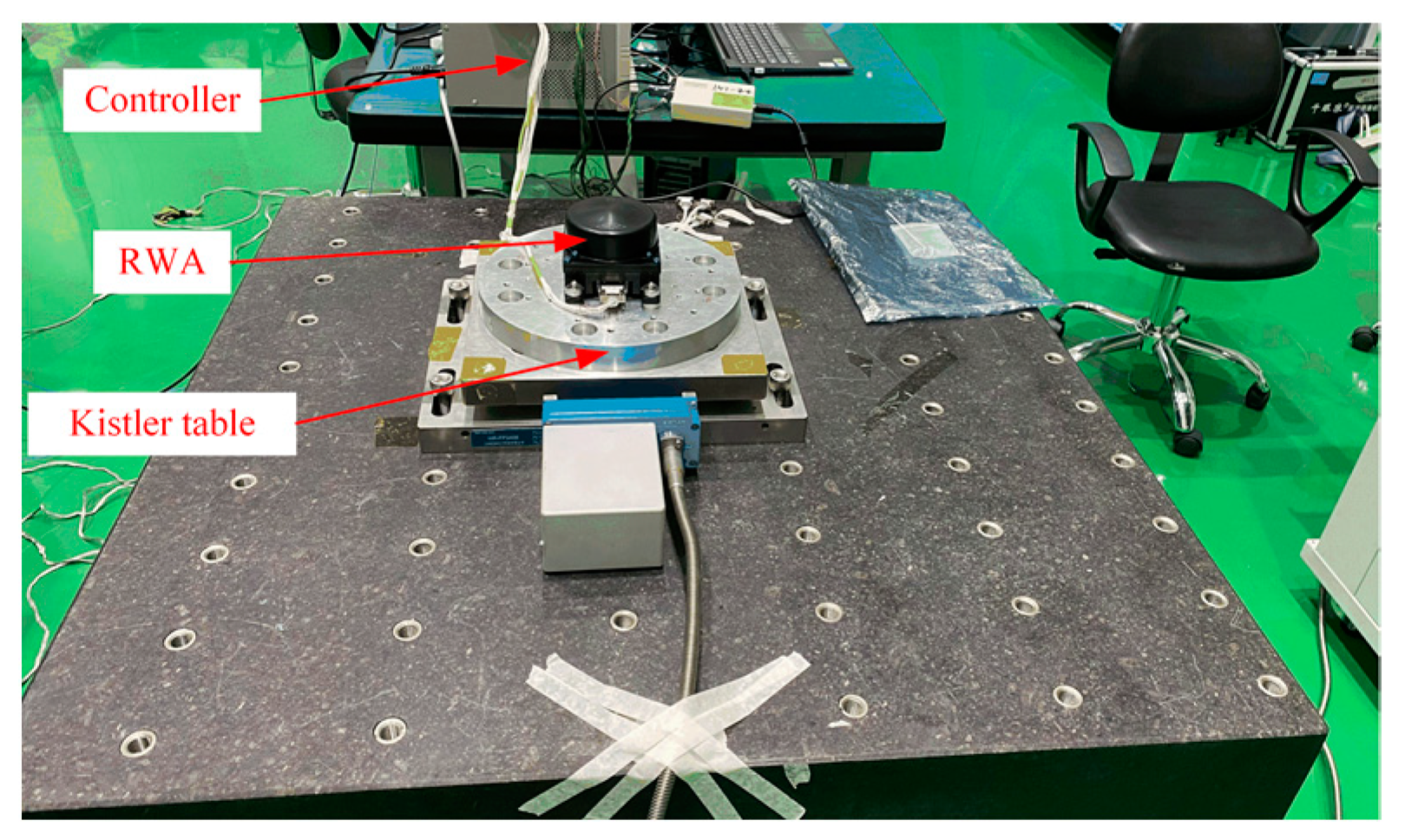
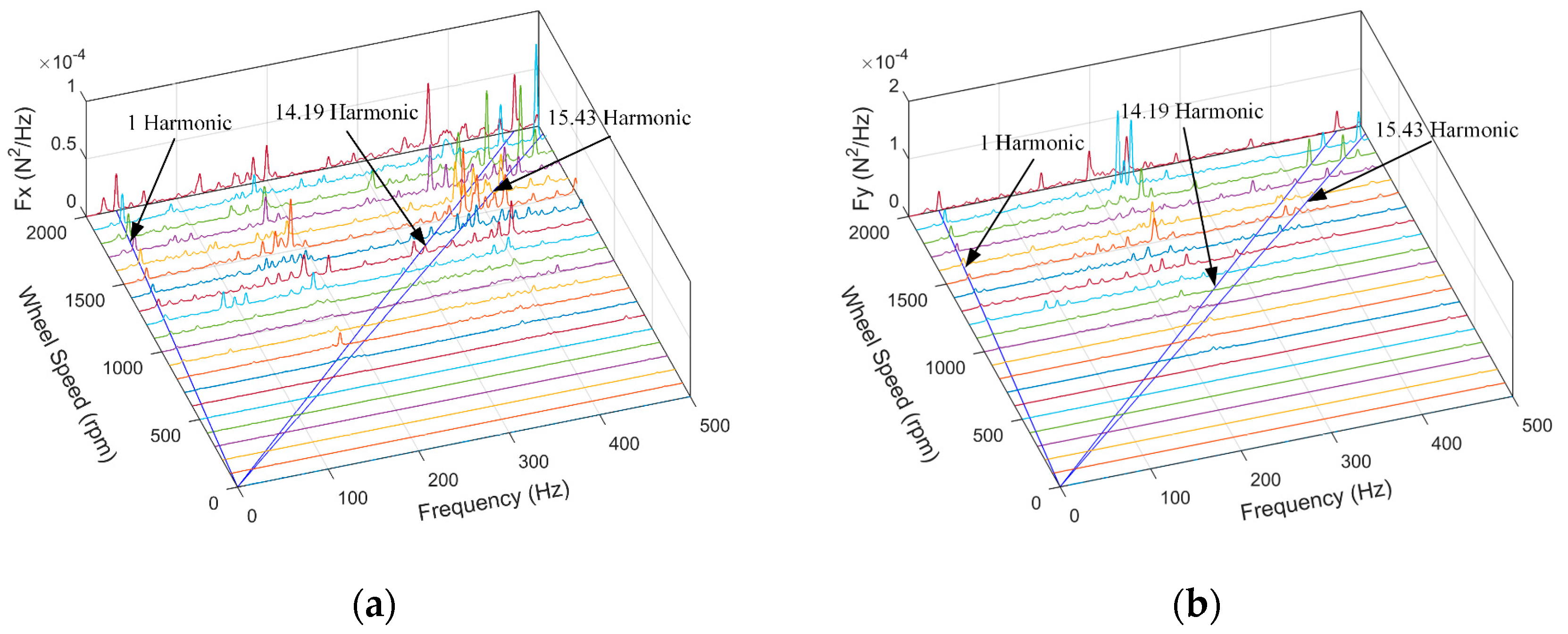
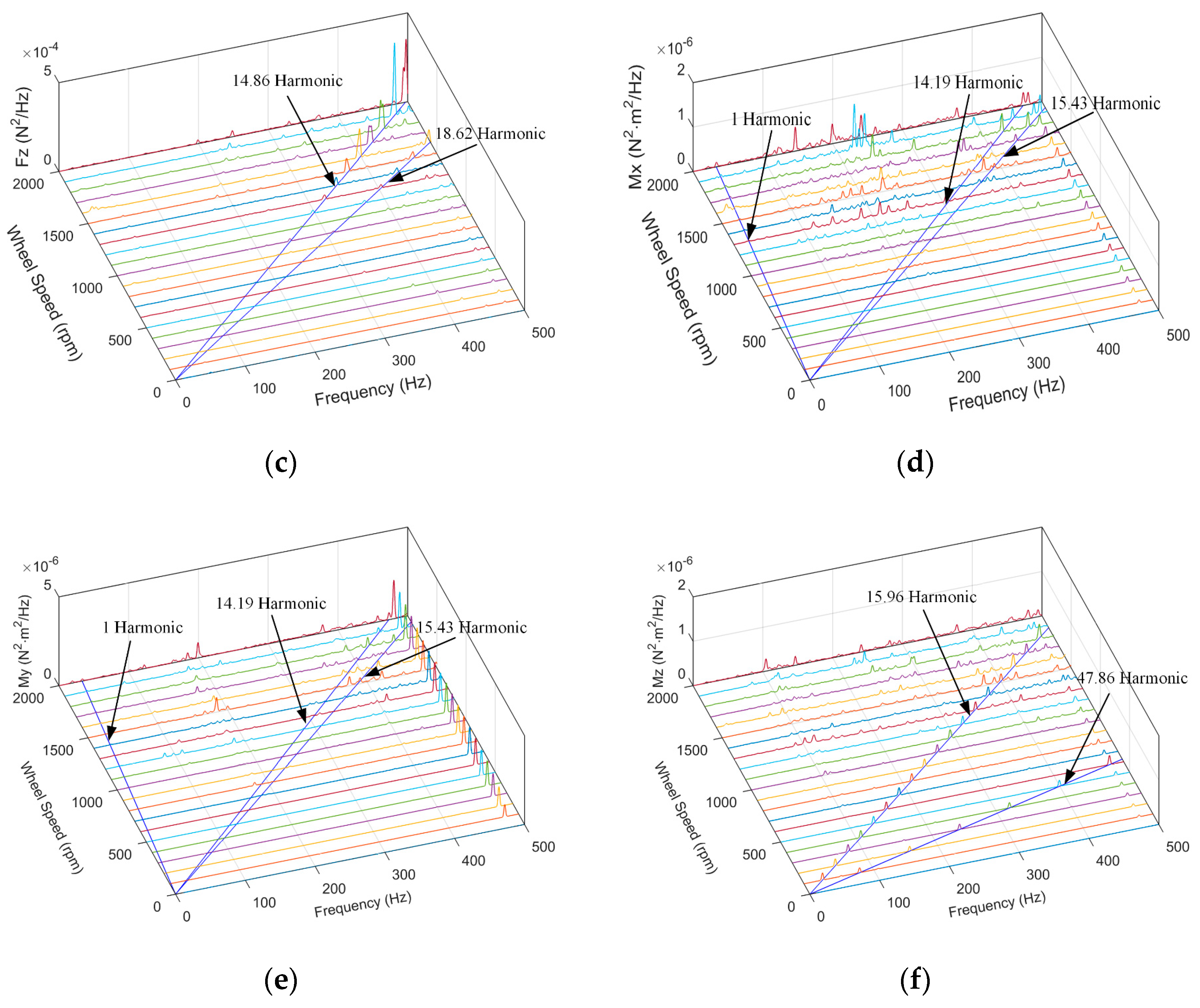
The disturbance force and tongue of RWA in the hard-mounted boundary condition can be obtained using a Kistler table, as shown in
Figure 4, while the results are shown in
Figure 5. It can be seen that the main harmonic numbers of
Fx,
Fy,
Mx, and
My are 1, 14.19, and 15.43, respectively, while the main harmonic numbers of
Fz are 14.86 and 18.62 and
Mz are 15.96 and 47.86.
2.2. Structural Dynamic Model
The general equation that governs the structural dynamics of the satellite can be written as:
where
M is the mass matrix,
C is the damping matrix,
K is the stiff matrix,
F is the disturbance force or torque, and
q is the displacement response. Use the mode shape matrix to convert the physical coordinates to modal coordinates as follows:
where
Φ is the mode shape matrix and
η is the modal coordinates.
Substituting Equation (4) and the second time derivative of Equation (4) into Equation (3), equates to:
The equations forming Equation (5) are coupled. To uncouple the equations, pre-multiply Equation (5) by the transpose of the mode shape matrix
ΦT.
By doing so, the mass, stiffness, and damping matrices are diagonalized. The modal (generalized) mass matrix and the modal (generalized) stiffness matrix are simplified to:
While the uncoupled form of the dynamic equations can be written as:
where the modal damping matrix is provided as:
Generally, the modal damping coefficients are different for every mode and typically vary between 0.1% and 3% for lightly damped space structures [
16].
The normal frequency matrix is denoted as:
Conversion of Equation (9) to the state space form is as follows:
2.3. Optical Model
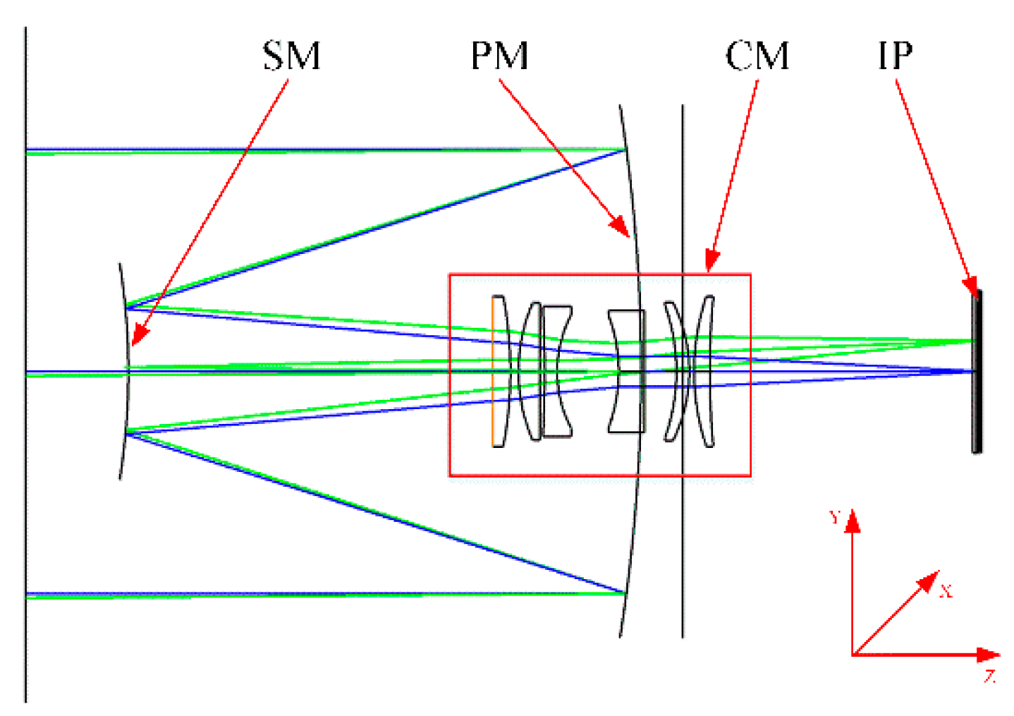
The payload of the satellite is an optical camera of Cassegrain type. The optical system is shown in
Figure 6. It is made up of a primary mirror (PM), a secondary mirror (SM), a calibration mirror (CM), and an image plane (IP).
The disturbance force and tongue will deform the optical component, which are usually small because it is very small. The deformation of each optical components can be considered a rigid-body motion. The best-fit rigid-body motion of the
ith optical element is defined as a vector
Ti of 6 terms as:
where
Tix,
Tiy, and
Tiz are translations along coordinate axes and
Rix,
Riy, and
Riz are rotations about coordinate axes. Then, the displacement of the node
j due to these motions is [
36]
where
xij,
yij, and
zij are the coordinates of the node
j, and
uij,
vij, and
wij are the displacements of the node
j. When there are
n nodes on each optical component, Equation (14) is expressed as follows:
where
qi = [
ui1,
vi1,
wi1,⋯,
uij,
vij,
wij,⋯,
uin,
vin,
win]
T, and matrix
Ai is expressed as follows:
The vector
Ti can be obtained from Equation (15) as follows:
where
Ci = (
AiTAi)
−1AiT. The matrix
Ci and
qi are functions of the coordinates and displacements of node
i, respectively. In order to ensure the accuracy of the fitting,
n is usually greater than or equal to 3.
The image motion
p(
t) can be obtained by summing the product of the rigid-body motions
Ti and the optical sensitivity coefficients
Li of the
ith optical element.
where
m is the number of optical components.
Li is defined as follows:
where
l11,
l12, and
l13 represent the image motions in the
x direction by translating the
ith optical component one unit displacement along the
x,
y, and
z axes, respectively. Further,
l14,
l15, and
l16 represent the image motions in the
x direction by rotating the
ith optical component one unit angle about the
x,
y, and
z axes, respectively. Moreover,
l21,
l22, and
l23 represent the image motions in the
y direction by translating the
ith optical component one unit displacement along the
x,
y, and
z axes, respectively. Finally,
l24,
l25, and
l26 represent the image motions in the
y direction by rotating the
ith optical component one unit angle about the
x,
y, and
z axes, respectively. The optical sensitivity coefficients of PM and SM, obtained by using the optical tracing method are shown in
Table 2, ignoring the CM and IP.
Substitute Equation (17) into Equation (18) and obtain:
where
qo = [
q1,…,
q2,…
qm]
T. Matrix
Co is expressed as follows:
2.4. The Integrated Model
Divide the degrees of freedom of the satellite into the degrees of freedom of the optical component
qo and the rest as
qr, as follows:
where
k is the number of modes.
Equation (23) can be obtained from Equation (22), as follows:
Substitute Equation (23) into Equation (20) and receive:
Rewrite Equations (12) and (24), and the integrated model of the satellite is provided, as follows:
3. FRF Estimation
Applying the Laplace transform of Equation (25), we acquire the transfer function
H(
s) from the disturbance to the image motion, as follows:
where
P(
s) and
F(
s) are the Laplace transform of
p(
t) and
F(
t), respectively.
Let
s = j
ω, then, we obtain the FRF
H(
ω). The relationship between the disturbance
F(ω) and the image motion
P(ω) in the frequency domain is:
where
F(
ω) = [
Fx(
ω),
Fy(
ω),
Fz(
ω),
Mx(
ω),
My(
ω),
Mz(
ω)]
T, and
H(
ω) is a 2 × 6 matrix.
In fact, when an RWA is installed on a flexible supporting structure, its disturbances excite the modes of the structure, which, in turn, perturb the RWA, itself, thus, creating coupled dynamics [
24]. As a result, the loads that are present at the interface vary from those that would be found in a hard-mounted boundary condition [
25,
26,
27]. The forces and moments
fC that are actually transmitted at the interface between the source and the supporting structure can be described as:
where
fB is the forces and moments measured in the hard-mounted boundary condition,
Dwa is the dynamic characteristics (inertia, stiffness, and damping) of the source and
ẍC is the vector of the coupled acceleration at the interface. The acceleration vector
ẍC can be determined if the supporting structure response at the interface node point (i.e., the dynamic mass of the supporting structure
Dss) is provided:
Substituting Equation (29) into Equation (28), Equation (28) can be rewritten as:
Rearrange Equation (30) and obtain
fC as:
where
I is a 6 × 6-unit matrix. Equation (31) can also be reformulated in terms of the Power Spectral Density (PSD) as:
where
fC and
fB become
ΦC and
ΦB, respectively, and H denotes the Hermitian transpose.
The PSD output of the image motion
Φout can be obtained by multiplying the
ΦC by the transfer function matrix, which links the interface node point to the image motion,
TFC−out, to obtain:
Due to the complexity of
Dwa and
Dss, many challenging experiments needed to be planned, similar to reference [
25]. The transfer function from
ΦB to
Φout is defined as:
The PSD output of the image motion
Φout can be rewritten as:
TFB-out can be obtained by the
Hv algorithm, by taking into account both the input and output noises [
28,
29,
30]. The following is a brief introduction to the
Hv algorithm. The augmented characteristic matrix
GFFX can be compiled as shown in Equation (34).
where
GFF and
GXX are the auto power matrixes of the input (disturbance force and tongue of RWA) and output (image motion in X direction), respectively.
GFX and
GXF are the cross-power matrixes of input and output. The singular value decomposition of
GFFX results in a diagonal eigenvalue matrix
Λ and an eigenvector matrix
V.
Choosing the column of
V representing the eigenvector, corresponding to the smallest eigenvalue and normalizing it, such that its last element is −1, the
Hv estimate can be obtained as shown in Equation (38):
when the augmented characteristic matrix becomes
GFFY, we can obtain [
H21,
H22,
H23,
H24,
H25,
H26] using the same method.
In order to reduce the estimation error of the FRF, geometrically average the FRF at different speeds, as follows:
where
Hij−k is the FRF
Hij at 100 × (
k − 1) rpm.
The coherence function is often introduced to evaluate the reliability of FRF. It is defined as the measure of the causal relationship between two signals with the presence of other signals. For the
ith output and the
jth input, the coherence function is formulated, as in [
28]
When the coherence function is equal to one, the two signals are completely related. If the coherence function between two input signals is 0, then, the two inputs are completely unrelated.
4. Experiment and Discussion
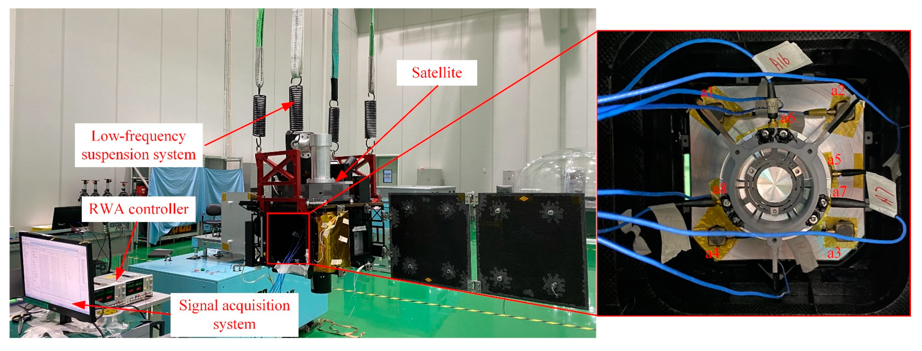
RWA is one of the most important disturbance sources on the satellite. We used the RWA disturbance as the excitation source to acquire the FRF from the disturbance source to the sensitive payload. The test platform of microvibration was built, as shown in
Figure 7, and mainly composed of the satellite, low-frequency suspension system, RWA controller, and signal acquisition system. Five acceleration sensors (numbered a1–a5) and three acceleration sensors (numbered a6–a8) were connected to the PM and the SM, respectively.
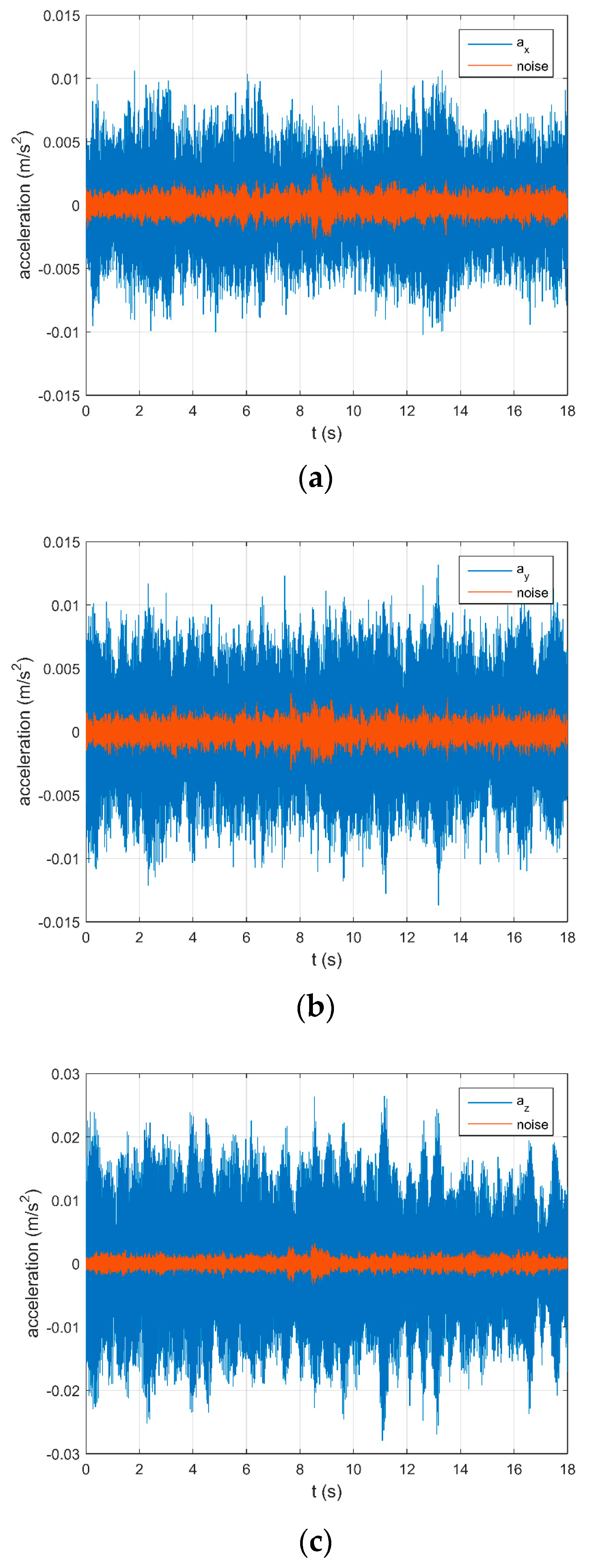
We collected the acceleration information of the 8 sensors, when the RWA increased from 0 to 2000 rpm, at every 100 rpm. The accelerations of a1 sensor in 3 directions at 2000 rpm are shown in
Figure 8. The figure shows that the test’s signal-to-noise ratio was high and satisfied the test requirements.
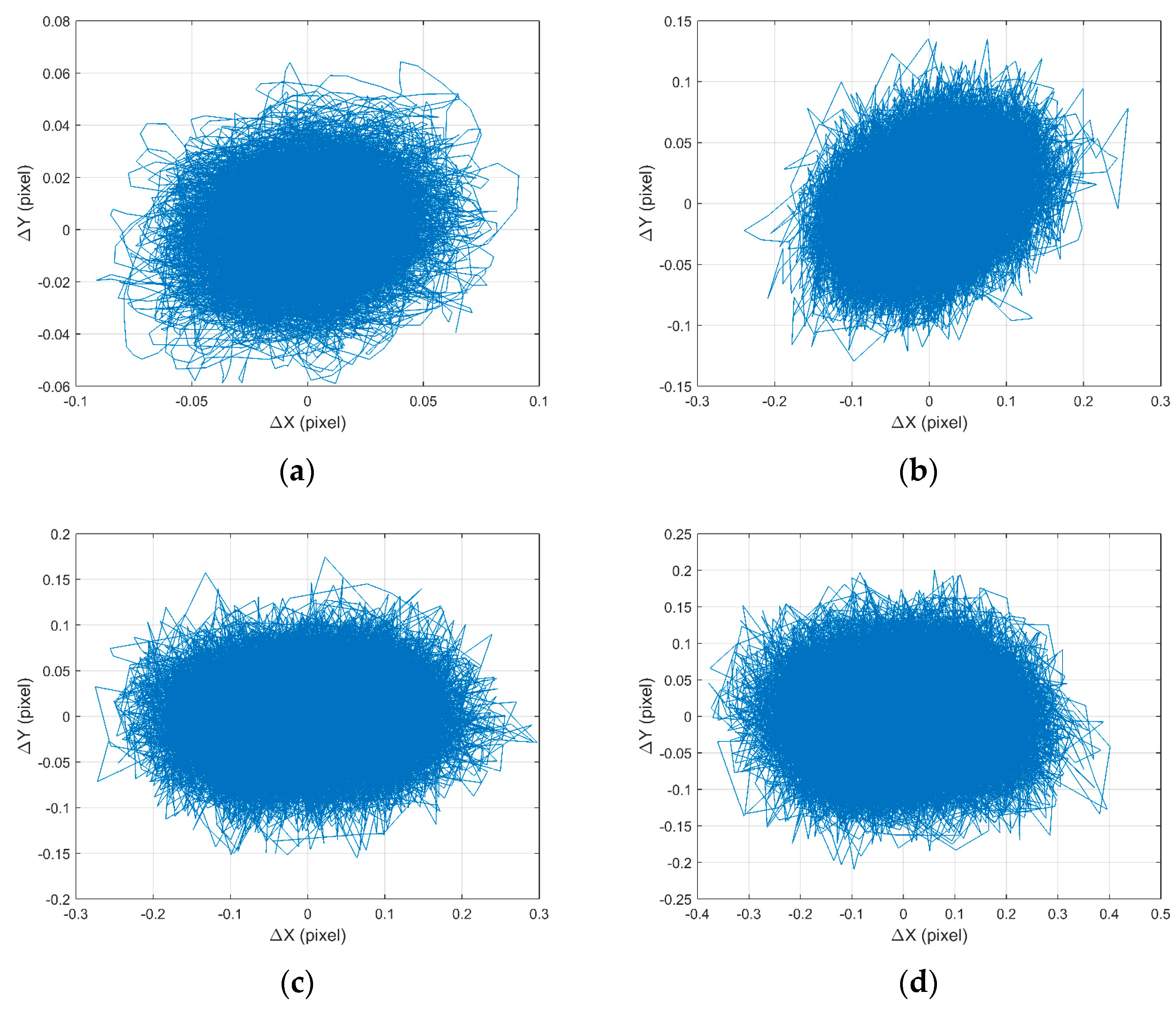
The gathered acceleration signals were transformed into displacement signals by quadratic integration, in order to fit the rigid-body displacement of each optical element, using Equation (17). Then, the image motion at each speed can be calculated by Equation (20). Through Equation (19), it is possible to determine the image motion at each speed, including the image motion at 0 rpm, 500 rpm, 1000 rpm, and 2000 rpm, as shown in
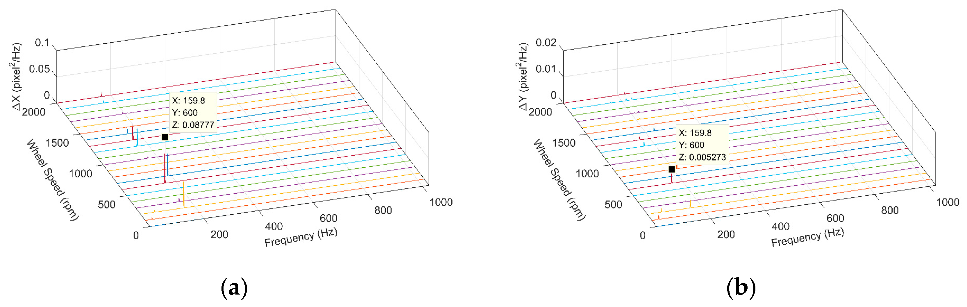
Figure 9. The waterfall of the image motion is shown in
Figure 10. The picture shows that when the RWA is at 600 rpm, there is a significant amplitude at 159.8 Hz.
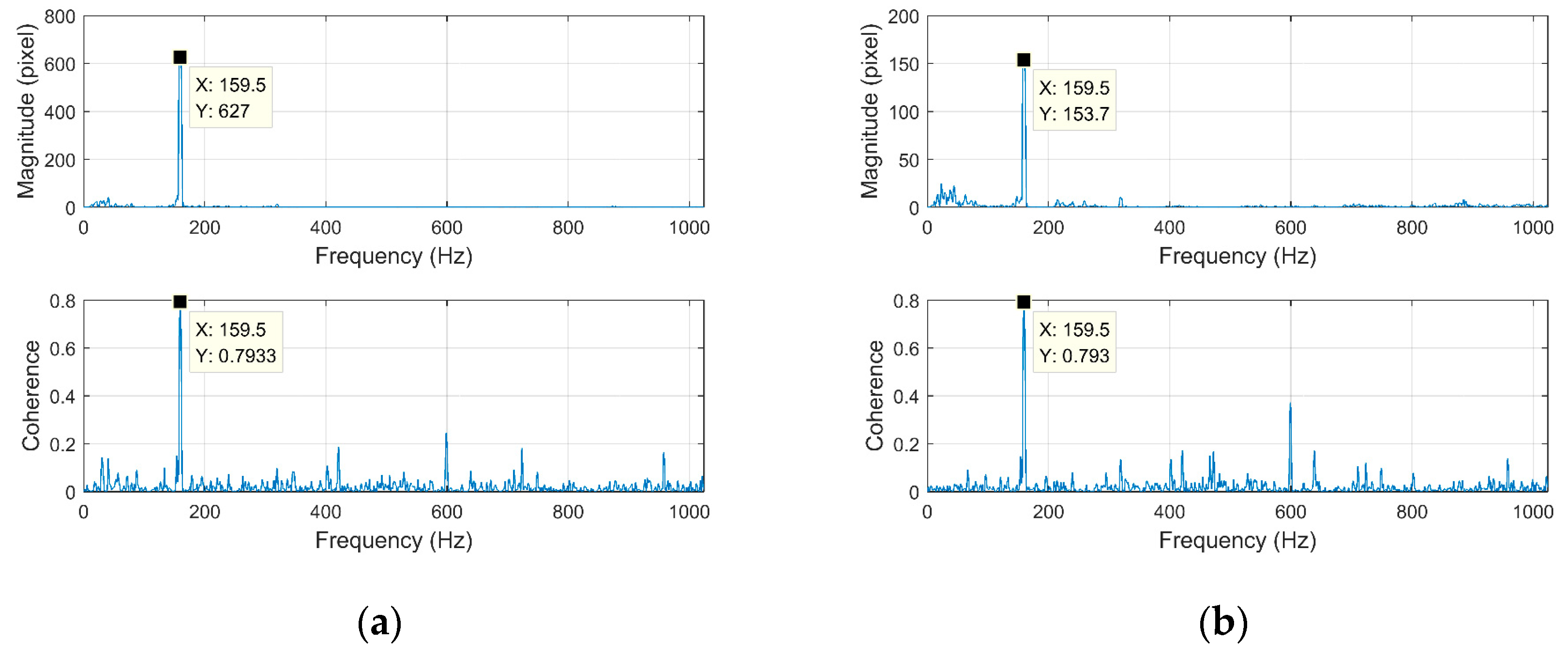
The FRF and coherence function at 600 rpm are shown in
Figure 11. For simplicity, only H
16 and H
26 are shown. The figure shows that the coherence at 159.5 Hz is roughly equivalent to 0.8, demonstrating the dependability of the FRF at this frequency.
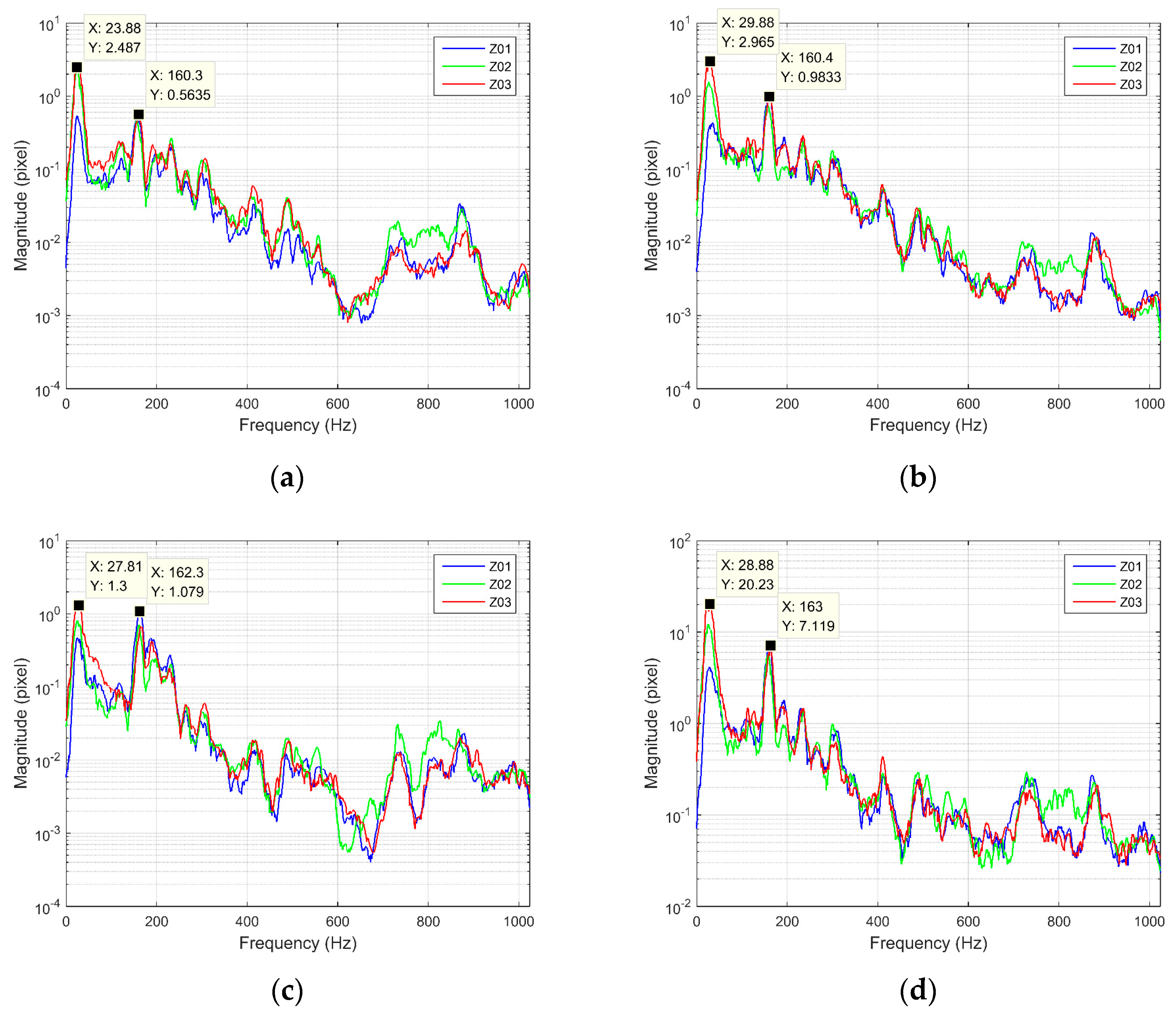
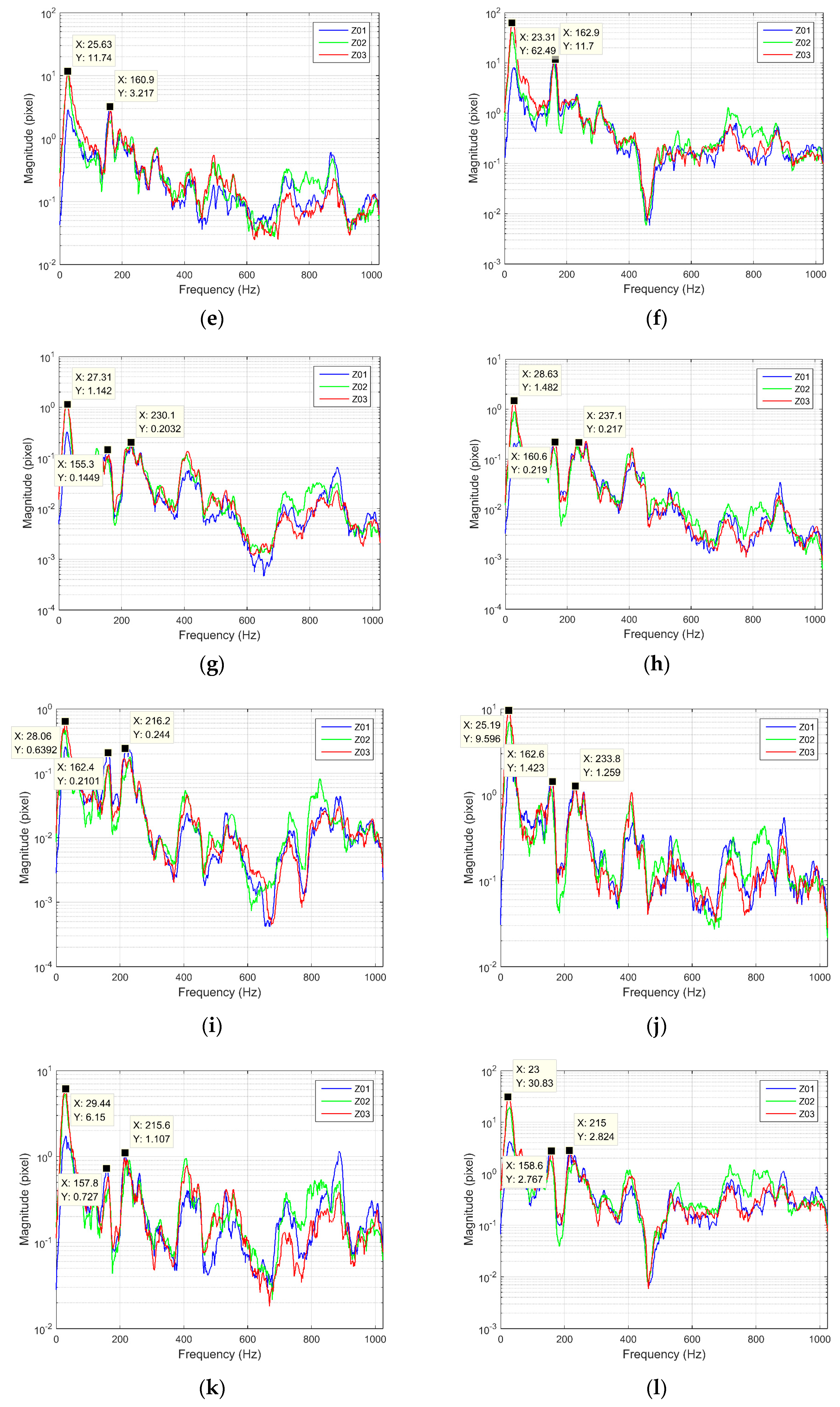
We can obtain the average value of the FRF at different speeds using Equation (39). We performed the same test using three distinct RWAs numbered Z01, Z02, and Z03, to validate the methodology suggested in this paper. The outcomes are depicted in
Figure 12.
As can be seen from
Figure 12, the amplitude of the FRF for the low frequency is larger, especially between 23 Hz–30 Hz, 155 Hz–163 Hz, and 215 Hz–237 Hz. Due to the influence of noise, the amplitude of the FRF obtained by different RWAs at 23 Hz–30 Hz differs greatly, while the differences at other frequencies are small. The figure also demonstrates that, at frequencies around 160 Hz,
Fx has the least impact on the image motion in the x direction compared to
Fz and
Fy, while
Mz has the greatest influence compared with
Mx and
My. Further,
Mz,
Mx, and
My have a decreasing impact on the image motion in the y direction, near 230 Hz, while
Fx,
Fy, and
Fz have the same effect.
5. Conclusions
In this paper, a general method that would obtain the FRF from the disturbance source to the sensitive payload was proposed. Firstly, the integrated model of a high-precision optical remote sensing satellite was developed, including the disturbance mode, structural dynamic mode, and optical mode, while the effect of AOCS was ignored. Secondly, a general method based on the Hv algorithm was presented to obtain the FRF, which does not require an additional excitation source, except for the RWA itself. Finally, a microvibration test of the satellite using different RWAs was carried out. The experimental results demonstrate that the coherence is high, and the peak positions of the FRF obtained by different RWAs are basically the same, while the amplitudes are slightly different, especially at 23 Hz–30 Hz, which indicates that the method proposed in this paper is effective. Therefore, the image motion of the sensitive payload can be obtained by multiplying the disturbance of the RWA measured at a fixed interface with the FRF, and without extensive testing when changing different RWAs in the same series.


 ,
, 


