Abstract
There are several index insurance methodologies. Most of them rely on linear piece-wise methods. Recently, there has been studies promoting the potential of data-driven methodologies in construction index insurance models due to their ability to capture intricate non-linear structures. However, these types of frameworks have mainly been implemented in high-income countries due to the large amounts of data and high-frequency requirements. This paper adapts a data-driven methodology based on high-frequency satellite-based climate indices to explain flood risk and agricultural losses in the Antioquia area (Colombia). We used flood records as a proxy of crop losses, while satellite data comprises run-off, soil moisture, and precipitation variables. We analyse the period between 3 June 2000 and 31 December 2021. We used a logistic regression model as a reference point to assess the performance of a deep neural network. The results show that a neural network performs better than traditional logistic regression models for the available loss event data on the selected performance metrics. Additionally, we obtained a utility measure to derive the costs associated for both parts involved including the policyholder and the insurance provider. When using neural networks, costs associated with the policyholder are lower for the majority of the range of cut-off values. This approach contributes to the future construction of weather insurance indexes for the region where a decrease in the base risk would be expected, thus, resulting in a reduction in insurance costs.
1. Introduction
Climate change has resulted in acute difficulties for low-income economies. Extreme weather events, such as droughts or heat waves, can cause crop failures and threaten the livelihoods of farmers and the food security of communities [1]. Mainly, these concerns can be severe due to underdeveloped financial services, where communities have access to limited financial services or even none at all [2]. Crop insurance is a tool that mitigates risk in farmers’ investments and is a growing market that reached USD36.6 billion globally in 2021 [3]. Globally, traditional insurance is one of the most widely used forms of protection for farmers, and traditional insurance calculates the indemnity by assessing losses after the occurrence of a weather event. However, it has two main problems: adverse selection and moral hazard [4]. Adverse selection occurs when there is a lack of symmetry in the information prior to establishing a deal between a buyer and a seller. A moral hazard occurs when there are fraudulent behavioural changes that might occur which could likely increase the risk of loss when a person knows that insurance will provide coverage.
An approach to mitigating risk is the use of index insurance which estimates the indemnity with an independent indicator of crop loss, such as a weather index [5]. In addition to reducing expenses, index insurance allows researchers to predict an individual farmer’s losses at different costs and different levels of accuracy [2]. The primary distinction between these different kinds of insurance is that the payoffs for the index insurance are determined by measuring weather variables [6].
Moreover, these types of insurance programs can also be beneficial for rural areas with social conflicts [7,8], as in the case of crop-productive regions in Colombia. Recent studies reveal that index insurance uptake reduces conflict risks caused by rangeland conditions by 17 to 50% and helps reduce poverty traps [9]. Therefore, social protection programs primarily represented by index insurance programs act as a protective factor in regions with complex risk profiles, where farmers are exposed to weather and conflict risks that may interact. This information is needed by governments to promote this type of insurance adoption.
When designing and implementing index insurance, it should also be recognized that it is vulnerable to high-basis risk due to imperfect relationships between the weather index and the risk it covers. Basis risk represents the difference between the payout or indemnity, as estimated by the weather index, and the policyholder’s actual losses [5]. This basis risk can take three forms: design, temporal, and spatial. Design basis risk occurs when the selected index does not correctly explain the target crop [5]. Temporal basis risk arises as a result of inappropriate period selection used to derive the index, while spatial risk arises from the spatial distance between the location where climate index data are collected and the location where losses occur [5]. Larger amounts of basis risk lead to high levels of remaining uninsured risk. Consequently, the index insurance contract is not cost-effective for farmers [10].
In Colombia, agriculture is one of the most important socio-economic sectors, accounting for 7.43% of the gross domestic product (GDP) in 2021 [11]. Agricultural land constitutes 35% of the national territory or 39 million hectares of land [12]. According to the National Administrative Department of Statistics (DANE by its Spanish acronym), 48.2% of the total agricultural production is concentrated in the departments of Antioquia, Valle del Cauca, Tolima, Cundinamarca, Meta, and Nariño, where agro-industrial products such as tubers, bananas, and cereals are grown [13]. Despite the sector’s importance, agricultural insurance in Colombia has a low penetration rate. As of 2014, only about 2.4% of the sown crop area of about 7.1 million hectares was insured [2]. Therefore, farmers are exposed to different types of risks and have to manage them.
There are few worldwide ongoing index insurance programs that use artificial intelligence and machine learning frameworks to derive insurance programs [5]. One example is the Pradhan Mantri Fasal Bima Yojana (PMFBY) program offered by the company Cropin [14]. As one of the big challenges in index insurance design is the availability of data, this company started in 2018 piloting small subplots within cultivated fields in five different states in India through the PMFBY program. The program relied on remote sensing with ground sensors and satellite images to measure yield performance among other crop development variables. One of the main goals of the program was to improve crop-cutting experiments (CCEs). Usually, CCEs are followed by inconsistent processes which can be translated into delayed and complicated yield data acquisition and forecasting processes [15,16]. Through artificial intelligence and machine learning techniques, the program provides reliable, cost-effective estimates of crop yields, which usually represents essential information in the conformation of index insurance programs. This program has benefited more than 250,000 villages across India.
In the case of Colombia, there is a lack of sufficient availability of crop yield data and other variables that measure soil and crop quality for index insurance research purposes. As crop production relies on high-dimensional weather conditions, the selection of weather variables for constructing the index insurance contract is crucial for the successful implementation of the hedging instrument. Moreover, crop development relies on weather conditions in a non-linear way [17,18,19]. Therefore, we propose an adaptation to an index insurance model in which we used a proxy variable for crop yield loss and satellite weather variables. This adaptation could be incorporated in further designs of index insurance contracts. We use neural networks to show that data-driven methodologies usually demonstrate superior performances to capture non-linear relationships in weather index insurance data. These models demonstrate their capability to capture the intricate relations between the weather variables and the loss, with the goal of lowering basis risk and costs and, therefore, increasing future willingness of farmers to acquire insurance.
According to Komarek et al. [20], risk can be classified into five types: production, market, institutional, personal, and financial. Production risk stems from the uncertainty associated with the natural growth process of crops, which is related to climatic events and pests [20]. Of the literature associated with weather insurance published from 1974 to 2019, 66% focuses on this type of risk [20].
Several methods have been employed in the literature to estimate the dependence between production and the index used. These methods seek to study the extent to which the variation in performance can be explained using the weather index. Rainfall and temperature are two of the most important factors that contribute to explaining variations in production [21]. Among these, the most widely used have been ordinary least squares regression and correlation [5]. Despite their frequent use, they have several drawbacks as they assume a constant relationship between all weather event scenarios and make assumptions that do not fit yield behaviour [5]. To overcome these drawbacks, QR, GAM, and copulas approaches have been explored for index insurance, which has been shown to be superior to OLS regression [5].
One approach to address the non-linear relationship between crop loss and the weather index is the implementation of machine learning models, which have great flexibility and can be adapted to complex information. Chen et al. [22], proposed a neural network-based design of an index insurance contract for production losses which helps to reduce basis risk and a utility function to derive the cost-effectiveness of index insurance. They found that the neural network-based solution had the optimal functional form of the insurance payouts, compared to other contracts such as linear, quadratic, and cubic piece-wise contracts; therefore, reducing basis risk. They used extensive datasets of annual corn production from Illinois from 1925 to 2018. The implementation of decision trees has proved useful in identifying important weather indices from satellite data [23] and for capturing non-linear relationships between different crop classes and low levels of precipitation, and evapotranspiration [5]. Additionally, Cesarini et al. [24] compare the performance of neural networks and support vector machines for identifying floods and droughts from satellite data, demonstrating the superiority of both methods over a logistic regression model [24]. There are other types of studies involving machine learning algorithms in weather index insurance. These are applied to crop yield predictions. Among them are You et al. [25] and Newlands et al. [26], who used neural networks to predict agricultural yields.
Although Colombia has low rates of penetration of weather index insurance, successful cases show that there is a potential for this type of insurance to be extended to more productive regions [2]. In this article, we aim to implement a machine learning framework to identify the best model for capturing the intricate relationships between weather variables and a proxy for crop losses. This represents an alternative method to traditional linear modelling that is used to derive insurance contracts. This methodology is applied in the Department of Antioquia, the largest agricultural producer in Colombia [13]. We used Python and Keras to implement artificial neural networks (ANNs). Keras is a high-performance application programming interface (API) from the TensorFlow library. This paper contributes to the state of the art as the application of machine learning methods has been limited in most low-income countries. This limitation has been shown even though machine learning methods have demonstrated their potential as non-linear and flexible methods for estimating performance–index relationships [24]. Furthermore, we believe that the research in index insurance programs should be promoted in low-income economies, especially in countries with social conflicts, as is the case of Colombia.
2. Objectives
Given that the application of data-driven methodologies for weather index insurance products, including machine learning frameworks in low-income countries, represents an important field of research in agricultural development [5], we have the following three goals.
First, a unique database from satellite images and flood records (the proxy for crop yield loss) from the department of Antioquia will be built.
Second, we want to compare a linear and interpretable model with a highly non-linear black-box model. Therefore, we will establish whether a machine learning model, such as the one recently used in the literature to model weather indices and loss [24], can be employed in a productive region in Colombia to establish if there is a relationship between weather indices and the observable losses due to floods. We used a logistic regression model as a reference point to evaluate the performance of a more complex model, ANN. The results from these machine learning models could serve to elucidate if the weather indices can better explain the losses in a particular agricultural region where sufficient crop yield data is not available.
Finally, using both the artificial neural network (ANN) and logistic regression models, we hope to assess the related costs for a hypothetical policyholder and an insurance provider. This could be used to derive fairer insurance policies before their implementation.
The main contributions are two-fold. First, we propose a novel way to implement an index insurance methodology by adapting a proxy variable to asses the crop losses in a country where no sufficient crop production data is available. Second, in addition to performance metrics, a utility measure is used to evaluate the performance of the ANN in relation to the base model, which is logistic regression.
Results obtained in this stage may be useful for the design of reliable indices for index insurance instruments with lower basis risk levels in low-income countries where agricultural and catastrophic data records are difficult to obtain. In this study, we use flood data records as a proxy of agricultural losses and satellite images for weather indices. We believe that the use of non-linear data-driven methodologies promotes the construction of fairer weather index insurance models in low-income countries.
3. Theoretical Framework
3.1. Machine Learning Algorithms
Machine learning is the science of programming computers to learn from data [27]. Machine learning models are classified into supervised and unsupervised. Supervised models are built on the expected response during training, so they learn by comparing the estimated output with the expected output. On the other hand, unsupervised models do not have an output variable during training, so their purposes include looking for patterns in the data or summarising the data into fewer dimensions.
Machine learning models are useful in complex contexts where traditional approaches cannot provide robust solutions. These models can also be implemented in fast-changing environments, as the models can be easily retrained and kept up to date [27]. The application of machine learning has increased in problems such as image recognition, language processing, speech recognition, and medical applications. This study uses neural networks, which are ideal for tackling complex problems due to their versatility and potential.
3.2. Artificial Neural Networks
Artificial neural networks (ANN) are the building blocks for deep learning approaches. Over the last decade, the area of machine learning and artificial intelligence (AI) has advanced greatly [28]. The term neural networks comes from the way algorithms tend to mimic how the human brain thinks. The way a neural network with one single layer works is based on the thousands of linear combinations which are fed from input variables. This information is later transformed by a non-linear activation function to obtain the output of the model. The final model is linear with respect to the transformed variables. One example of an ANN with one single layer is depicted below in Figure 1.
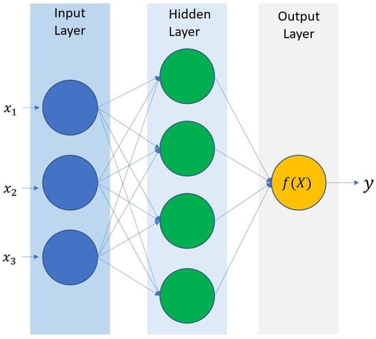
Figure 1.
Artificial neural network of one single layer. Source: authors.
The output of an ANN with one single layer is [28]:
where are the activations of each unit of the hidden layer:
The function g is the activation function that must be defined previously. One of the most common activation functions is the ReLU function. The non-linearity of the activation function is essential to capture the non-linear effects and interactions among the network [28]. It is required to define a loss function to adjust the model. Therefore, a gradient descent algorithm is applied to adjust the weights on each of the layers of the network.
In this study, we used Python’s library Keras to implement the ANN. Keras is a high-performance API from the TensorFlow library. Keras allows us to build and train the ANN. It additionally has the ability to optimize GPU computational loads.
3.3. Performance Metrics
ANNs for classification tasks usually generate two types of predictions. One is a continuous prediction, usually in the form of a probability output. Another is a discrete prediction, which generates a class. In practical applications, categorical predictions are usual as they ease decision-making. However, probability outputs for continuous predictions are useful when assessing the model’s performance and reliability according to a known class [29].
One common method to assess the performance of a classification model is through a confusion matrix. This method relies on a table which is a summary of the number of correct and incorrect predictions made by a classifier. The diagonal elements show the observations for which the class is predicted correctly, whereas the rest of the elements show the two types of errors that are present in classification problems; particularly false negatives and false positives (Figure 2).
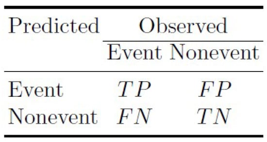
Figure 2.
Confusion matrix [29].
Despite the use of a confusion matrix to assess a model’s performance in a classification ANN, when there are thousands of configurations, it is necessary to use a univariate metric to assess the performance of the ANN model. If one of the classes is considered as one of interest, it is possible to use metrics such as precision, sensibility, and specificity to summarize part of the information in the confusion matrix [28].
There are other metrics to assess other components of the matrix such as the accuracy and F1 score. The accuracy metric measures the relationship between the observed and predicted classes, and it is easy to interpret. However, there are some disadvantages in its use. For example, it is incapable of distinguishing between the type of errors (false positive or false negative), and it can be unreliable when there are unbalanced classes [29].
On the other hand, the F1 score measures the harmonic media between precision and sensibility [24].
Another way to measure the model’s performance is through probability prediction which can potentially provide more information than the simple value of the class [29].
The curve “receiving operator characteristic” or ROC, is a chart that uses the rate of true positives (sensibility) against the rate of false positives (1-specificity) for the range of probabilities. A perfect model would have a specificity and sensibility of 100% for all the probability ranges, and the area under the curve (AUC) ROC would be 1. On the other hand, there is the PS curve, which is obtained by plotting precision against sensibility. In this case, the AUC could be used to measure the model’s performance [28].
3.4. Index Insurance
Traditional insurance tools assess the risk to the insured. One of the main risk factors in agriculture is the weather, which is a correlated risk. This means that when an event occurs, many policyholders are affected simultaneously [30]. This situation can involve high costs and is a critical factor for the financial viability of these insurances as a single event could result in losses that exceed the available capital if careful planning is not carried out [4].
Unlike traditional loss-based insurance, index insurance pays out to the holder according to a predefined index which is highly correlated with a loss variable [4]. These indices are based on specific measures, such as precipitation or temperature, which can show a clear correlation with a response variable such as crop production, yield production, or a proxy of both. One of the advantages of index insurance is that it exhibits lower costs compared to traditional loss insurance. For example, lower transaction costs which makes it potentially more affordable in low-income economies [4].
4. Methodology
Index insurance indemnifies the policyholder based on the observable value of the predefined index which is highly correlated with losses. There are values or thresholds which define the trigger signal of indemnities. In the context of machine learning, this corresponds to a classification problem, allowing researchers to predict the occurrence of a loss event. In this study, we use historic flood data as a proxy of losses. Particularly, we use two data-driven methodologies to model the relationship between the loss occurrences with weather indices. The purpose of these models is to determine the occurrence of flood events based solely on the selected weather indices values. The time period used to train the models extends from 3 June 2000 to 31 December 2021. The starting date was selected due to the historical availability of the GPM time series (Table 1), while the end date was selected due to the lack of availability of data in the flood record database.
Results obtained by Figueiredo et al. [31] showed that logistic regression models provide good results when explaining loss events through weather indices. However, given that this is a linear model, its predictive capacity is significantly limited when compared to more flexible models. Thus, logistic regression was used as a base model to provide a reference point when assessing the performance of a more complex model, namely ANN. Given that the goal is to compare a linear and interpretable base model with a highly non-linear black-box model, other possible non-linear models, such as decision trees and support vector machines, are not considered.

Table 1.
Characteristics of the selected (quasi-)global precipitation databases.
Table 1.
Characteristics of the selected (quasi-)global precipitation databases.
| Database | Type | Resolution | Frequency | Coverage | Time Lapse | Latency | Reference |
|---|---|---|---|---|---|---|---|
| CHIRPS | Satellite | 0.05° | 1 d | 50° S–50° N | January 1981–Present | 3 weeks | [32] |
| estimation | |||||||
| PERSIANN-CDR | Satellite | 0.25° | 1 d | 60° S–60° N | January 1983–Present | 48 h | [33] |
| [34] | |||||||
| GPM | Satellite | 0.10° | 30 min | 60° S–60° N | June 2000–Present | 12 h | [35] |
The particular aim of applying highly non-linear models is to lower the basis risk in future designs of index insurance instruments.
Consider the occurrence of floods caused by weather events for each time unit for a region G, where is a binary variable such as:
The objective is to predict the likelihood of a flood event using weather variables from satellite images. The model has a probabilistic variable output which is used to optimize the cut points in which indemnities are disbursed. This last step is performed from a two-party perspective, considering that both parties have different costs.
Moreover, probabilistic outputs can also provide an uncertain measure that can be used by final users once the model is implemented [31].
Figure 3 summarizes the methodology used in this study which is adapted from two recent methodologies: Cesarini et al. [24] and Figueiredo et al. [31].
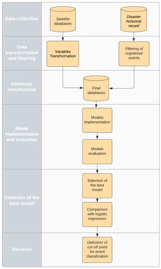
Figure 3.
Project M = methodology flowchart.
4.1. Data
4.1.1. Data Sources
According to [27], the performance of a model can be affected by selecting a “bad algorithm” or “bad data”; in addition, for most machine learning algorithms, a considerable amount of data is needed for them to work well [27]. For the specific case developed, selection criteria were implemented to build a representative database of the problem. Additionally, some of the selected predictors were proven to be significant in previously developed research, such as the database selected by Cesarini et al. [24].
Satellite data: Regarding satellite data, the Google Earth engine was used. It is a cloud-based geospatial tool that allows for the analysis of satellite images. Cesarini et al. [24] used a criteria to select data sources and to implement a tool that could be used in the context of parametric risk financing tools. These are summarized below:
- Spatial resolution. A precise spatial resolution that takes into account the different climatic characteristics of the area of interest is necessary to develop accurate parametric hedging products.
- Frequency. The datasets selected should be commensurate with the duration of the event of interest. In the case of floods, which are rapid phenomena, daily frequencies or lower temporalities are required.
- Spatial coverage. Global coverage allows for the extension of the developed approach to areas other than the region of interest.
- Temporal coverage. Since extreme events are infrequent, a spatial coverage of at least 20 years is necessary for correct model calibration.
- Latency. A low latency time (i.e., time delay until the most recent data is obtained) is necessary to develop tools capable of identifying extreme events close to real-time.
Based on the criteria, and restricting the search to databases available in the Google Earth engine, three precipitation databases and a database with a surface run-off variable, and four soil moisture levels were selected. The use of multiple databases allows researchers to improve the ability of the models in capturing extreme events [24]. The selected datasets for precipitation came from Climate Hazards Group InfraRed Precipitation with Station data (CHIRPS), Precipitation Estimation From Remotely Sensed Information Using Artificial Neural Networks-Climate Data Record (PERSIANN-CDR), and Global Precipitation Measurement (GPM) (Figure 4, Figure 5 and Figure 6). The CHIRPS data (Figure 4) shows the most extreme differences in precipitation levels. The central and north regions present lowest values (1000 mm per year). In the other hand, the east and southeast regions present the highest precipitation levels (5000 mm per year). The PERSIANN (Figure 5) and GPM (Figure 6) figures show the same configuration of precipitation values, but with different resolutions.
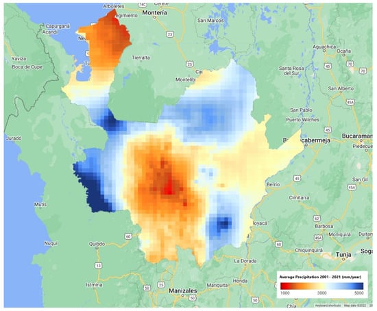
Figure 4.
Precipitation values in Antioquia Department, Colombia by the Climate Hazards Group InfraRed Precipitation with Station data (CHIRPS).
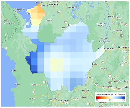
Figure 5.
Precipitation values in Antioquia Department, Colombia by the Precipitation Estimation From Remotely Sensed Information Using Artificial Neural Networks-Climate Data Record (PERSIANN).
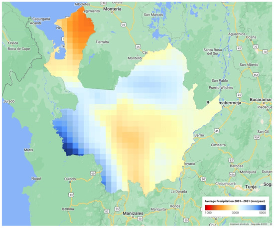
Figure 6.
Precipitation values in Antioquia Department, Colombia by the Global Precipitation Measurement (GPM).
On the other hand, for the run-off and soil moisture variable, the ERA5 dataset was used, which is produced by the European Centre for Medium-Range Weather Forecasts (ECMWF). The main characteristics of the datasets are shown in Table 1 and Table 2.
Table 2.
Characteristics of the selected global database for soil moisture and surface run off.
4.1.2. Flooding Record
The flooding records correspond to the model’s output variable. This variable represents the consolidated historical record of emergencies produced by the National Unit for Disaster Risk Management (UNGRD) [37,38]. This entity guides the National Disaster Risk Management System and manages the implementation of risk management, policies, and compliance with internal regulations, as well as the functions and duties established in Decree 4147 of 2011. Based on the historical record, only the events of interest were filtered; in this case, reported floods from the records from the department of Antioquia. The data comprises the natural disasters reported from 1998 to 2021.
4.1.3. Data Transformation
Flood damage is not directly caused by precipitation but by actions caused by the flow of water. Thus, even if floods are related to rainfall, rainfall by itself is not the best predictor of the intensity of a flood [31]. Therefore, a transformation is adopted that seeks, in a simplified way, to emulate the process by which floods are caused due to rainfall. This is based on an approach proposed by Figueiredo [31].
First, because part of the rainfall water is absorbed by the land, a parameter is adopted that represents the daily infiltration rate. Then, the rainwater that is not absorbed (run-off) is defined for the cell as:
In addition, the flow of water over the surface accumulates due to excess rainfall. For this reason, this behaviour is represented by a weighted moving average, which is restricted to 3 days. The cumulative surface flow (cumulative run-off) for the cell during days t, and is given by:
where and .
Finally, a summation is performed over the region of interest to summarize the information in a single variable with a daily time period.
4.1.4. Data Preprocessing
Data pre-processing refers to the addition, removal, or transformation of training data. Data preparation can make or break a model’s predictive ability. Different models have different sensitivities to the type of predictors used [29]. In the case of neural networks, the scale of the predictors can have a large effect on the final result [28]. For this reason, it is best to standardize the predictors to have a mean zero and a variance of one.
For most machine learning techniques, a little imbalance is not a problem; however, if the imbalance is high, the standard optimization criteria or performance metrics may not be as effective as expected [24]. There are several methods to counteract the negative effects of class imbalance. Among these are post hoc sampling methods, which are based on selecting a training sample with approximately the same event rate for both classes. Among the sampling techniques, there are two general approaches, oversampling and undersampling [29]. Additionally, there are techniques such as the “synthetic minority oversampling technique” (SMOTE), described by Chawla et al. [39], which selects a point at random from the minority class and generates a new point from its k nearest neighbours.
4.1.5. Selection of the Best Model
When modelling a classification problem, the relative frequency of classes can have a significant impact on the effectiveness of the model [29]. The imbalance of classes can even affect the evaluation metrics, which can be misleading when evaluating the performance of a model, possibly resulting in the selection of a poorly designed model [24]. Both the ROC curve and accuracy should be used with caution when working with unbalanced classes [24] because a high number of true negatives tend to result in low false positive rates (FPR = 1 − specificity).
4.1.6. Result Validation
In addition to assessing the quality of a model, based on performance metrics, it is possible to assess the utility of the model, i.e., the economic value it brings to the end user. In fact, a measure of value is even more important than a measure of quality since users are primarily concerned with the estimated benefit that models can bring in the context of the problem [31]. To evaluate the usefulness of the implemented models, we follow the methodology implemented by Figueiredo [31] which is summarized below.
Table 3 shows the frequencies of the four possible combinations of predicted and occurring events.
Table 3.
Event frequency for each case.
Each component of the table has an associated cost, which can be expressed in the form of a cost matrix (Table 4).
Table 4.
Event costs for each case.
The average cost of using a certain predictive system can be obtained by multiplying the relative frequencies and associated costs.
Although this equation allows researchers to calculate the average value, it is also useful to calculate a measure of the benefit obtained by using the predictive system. Thus, a reference or base system is defined, for which a system that never predicts a loss event (flood) is assumed. In this case, the average cost is given by
where
The value is then defined as
In addition, the average cost associated with a perfect forecasting system, for which the predictions and the observed events always agree, is defined. The cost of this system is given by
which corresponds to the upper bound on the maximum value that can be obtained from a system.
By presenting the predictions in probability form, the end user is faced with the possibility of selecting the cut-off point q that maximizes the value they can obtain from the system. Varying the cut-off point from 0 to 1 allows a sequence of values to be computed, from which the optimal decision can be found.
The model is evaluated from the perspective of two users of a hypothetical parametric insurance product. This includes the policyholder and the insurer.
The cost matrices associated with each of the parties are then defined. For the insured party, in this case, the Antioquia region, is defined as the expected indemnity in the event of a loss event (flood). It is assumed that the indemnity corresponds to the expectations of the department, so there is no net gain or loss for the insured party. The premium to be paid by the department is defined as follows:
where m corresponds to the insurer’s relative profit margin (). Finally, assume that represents the losses incurred by the department in case a loss event occurs but no indemnity is generated.
Now, the costs of the second party, the insurer, are defined. Assume that corresponds to the operational costs related to administrative actions each time an indemnity is generated, corresponds to the reputations and model recalibration costs generated each time an indemnity is generated but no event occurred, and is the reputation cost and the potential loss of a customer each time the model fails to generate an indemnity when a loss event occurs.
The cost matrix for both parties is shown in Table 5. From this table, the average cost of each of the parties associated with a value q can be found.
Table 5.
Cost of events for the users.
For parametric risk financing products, only one cut-off point can be selected in the policy conditions [31], and it is possible that no single cut-off point is optimal for all parties involved. However, according to Figueiredo [31], the framework implemented to calculate the value associated with the predictive system provides a way to make decisions regarding the cut-off point that is beneficial to all users.
To validate the results obtained, a comparison is made between the best machine learning model and the best logistic regression model of the value associated with the optimal cut-off point for each of the parties.
5. Results and Discussion
The results are presented next. The first part refers to model building and then the performance and selection of the models are carried out, including insights into the costs for both parties.
In model building, there are multiple hyperparameters, such as the loss function, the optimizer used, the number of layers and nodes, and the activation function. Each of these hyperparameters can be chosen from a large number of options, but there is no clear indication of the number of hidden layers or nodes that should be used for a specific problem. According to James [28], it is currently considered that the number of units per layer can be high, and over-fitting can be controlled by making use of the various forms of regularization. Accordingly, the space of configurations for the neural network must be limited, since it is practically infinite. For this reason, a range of values was selected for each of the hyperparameters of the model, which are summarized in Table 6.
Table 6.
Explored configuration space.
A space of 27,000 configurations is explored, using 15 combinations of the data series. The selected combinations were chosen as follows:
- 1.
- Possible combinations from two to four precipitation data series of indices were tested. Specifically, the three precipitation data series and the surface flow data series. This results in 11 possible combinations.
- 2.
- Subsequently, each of the soil moisture levels were added sequentially. This corresponds to 4 additional combinations of the model inputs.
Referring to the pre-processing techniques, there was a severe class imbalance, where the ratio of the minority class to the majority class was approximately 1:16. For this specific problem, oversampling, SMOTE, and a mixture between undersampling and oversampling were selected as pre-processing techniques, specifically to improve the sensitivity of the implemented models.
Regarding the selection of the best models and in line with the methodology used by Cesarini [24], we used several performance metrics: F1 score and the area under the precision–sensitivity (PS) or the AUC score. Additionally, we used a utility measure to derive the optimal cut-off point which also serves to derive the costs related to each model. When using two metrics, they will not necessarily coincide when selecting the best model, so the models selected with an F1 score are analysed first, followed by those selected with the AUC. In this study, we used a logistic regression model as a baseline to compare the performance of the best models.
Therefore, the performance of the models shows that when using:
- F1 score as a selection criterion: the best model is obtained using seven datasets, a combination of undersampling and oversampling as a pre-processing technique, one hidden layer, and ReLU as an activation function. The hidden layer’s dropout rate is 0.4. This architecture corresponds to a simple neural network, with an intermediate level of regularization.
- The area under the precision–sensitivity curve (AUC): the best model uses seven input datasets, a mixture between undersampling and oversampling as a pre-processing technique, four hidden layers, and the ReLU activation function. The dropout rate for each layer is 0.0, 0.6, 0.6, and 0.6, respectively.
On the other hand, when comparing the best model architectures with those obtained by Cesarini [24], it is evident that the model complexity here studied is significantly lower than the one obtained in that study. Even though deeper structures were explored, results showed poorer performance metrics due to possible overfitting during training. This low performance may happen for several reasons. One possible failure in the reporting processes for catastrophic events in low-income economies, such as the one studied here for flood events, is a possible lack of coherence between the actual flood date and the reported one. As mentioned by Géron [27], the performance of a model can be affected by using poor data as is the case here.
Figure 7 shows the performance of the best 27 configurations in the precision-recall space, which also includes level curves corresponding to the F1 score. The precision–sensitivity curve allows each model to be evaluated for the whole range of cut-off probabilities. The perfect model resides in the upper right corner, with a precision and sensitivity of 1. Based on this result, the performance of the best models is far from the optimal model and closer to the baseline model.
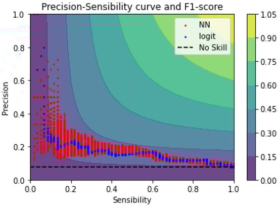
Figure 7.
Top 0.1% configurations according to F1 score.
The best performance of the neural network models is associated with an F1 score of 0.2989, while the logistic regression model achieves a maximum F1 score of 0.2739. Regarding the AUC metric, the machine learning model achieves a score of 0.214, while the logistic regression model achieves an AUC score of 0.205. Table 7.
Table 7.
Model comparison, F1 score selection.
Figure 8 compares the F1 score evaluated in the test data for an increasing number of input datasets. Neural network results were averaged for three iterations, due to the stochastic component related to model training.
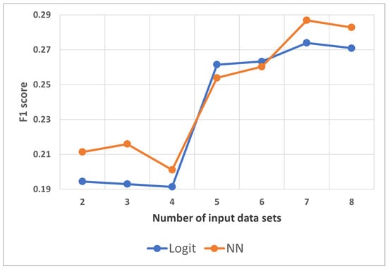
Figure 8.
Comparison test F1 score, ANN and logistic regression.
Regarding the indices that better explain the losses, the results show that the machine learning algorithm achieves a better result, but its performance is not superior in all cases. The selection of datasets was performed as mentioned earlier, where the first four datasets correspond only to precipitation and run-off data, and the last four datasets are the different soil moisture levels. In Figure 8, a significant jump can be observed when the first soil moisture level is included, which indicates an improvement in the predictive capacity of both models.
As previously stated, we also used AUC as a selection metric, where we derived the best model and compared its performance with a logistic regression model. Figure 9 shows that the machine learning model achieves an AUC score of 0.23, while the logistic regression model achieves an AUC score of 0.20.
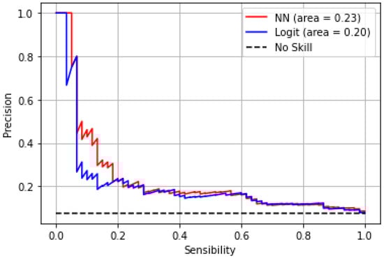
Figure 9.
Precision-recall.
Figure 10 shows the F1 score for the range of cut-off probabilities. The neural network model achieves a higher F1 score than the linear model for almost the entire probability range. The curve related to the machine learning model is generally above the curve of the linear model, which indicates that it generally performs better for the range of cut-off probabilities. On the other hand, similar models [24] achieve higher performance metrics for the F1 score and AUC score. However, the methodology presented here supports the idea that machine learning methodologies perform better than logistic regression which represents a traditional classification framework.
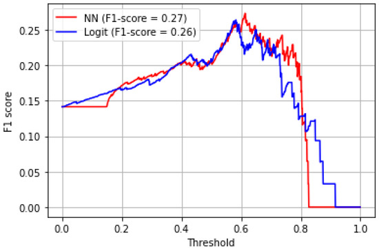
Figure 10.
F1 score.
As mentioned earlier, a hypothetical utility measure is computed for both parties (policyholder and insurance provider), which could be used to derive the optimal cut-off point and compare the costs related to each model. Therefore, we followed the procedure mentioned in Section 5 First, the various costs associated with the parametric model must be defined. The following parameters are used: = $1,000,000; = $2,000,000; m = 1.15; = $5000; = $20,000; = $350,000. Figure 11 and Figure 12 show the average cost associated with the best model selected using the F1 score, comparing its performance with the cost associated with a linear model. Results show that the curves associated with neural network models have lower costs than the logistic regression model for almost the entire range of probabilities. As for the insurer, the logistic regression model achieves the lowest cost. However, the neural network models generally present lower costs for almost the entire range of probabilities.
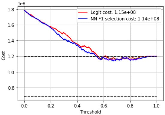
Figure 11.
Policyholder-related costs.
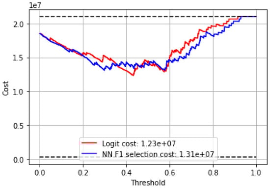
Figure 12.
Insurance provider-related costs.
6. Conclusions
In this study, we employed two data-driven frameworks to assess the relation between three weather indices: precipitation, run-off, and soil moisture. We used flood records as loss events. This adds nuance to the building processes of index insurance models, particularly in the field of basis risk and its reduction. We used data from the period between 3 June 2000 and 31 December 2021 from the department of Antioquia, Colombia. We used flood records as a proxy for crop production loss, which is the traditional variable in index insurance models because agricultural data in Colombia is difficult to obtain or in many cases, non-existent.
We implemented a similar methodology to Cesarini [24], by using neural networks and logistic regression frameworks and by using the F1 score and AUC score for the selection of the best models. Results show that neural networks with one hidden layer, 100 hidden units, 0.4 dropout rate, and the ReLU activation function performs better than traditional logistic regression models for the data used. Even though the F1 score and area under the precision–sensibility curve metrics perform better than logistic regression, performance metrics are lower than the state-of-the-art architectures. However, these results are coherent with previous studies that indicate that data-driven methodologies, such as neural networks, tend to perform better than traditional methods for explaining the relationships between the weather indices and the losses in index insurance models.
Perhaps, one of the biggest restrictions in data-driven studies is the quality and availability of data. As is the case for low-income economies, low-performance results could be explained by the quality of the data, where one possible cause of such results could be related to the reporting processes for the catastrophic events in the region studied, in this case, the flood records.
To support the selection process for best model performance and to understand related costs in a weather index insurance contract, we applied a utility model to derive a measure for the costs associated for both parties involved: the policyholder and the insurance provider [31]. A measure of value is more relevant than a measure of quality, as the end users are more concerned with the estimated benefits associated with the context of the problem. Results show that costs associated with the policyholder are lower for the most part of the range of cut-off values. This is related to an improvement in the predictive capacity of the model, which is in line with a reduction in the basis risk. This approach contributes to the future construction of weather insurance indices for the region where a decrease in the base risk would be expected and, thereby, a reduction in insurance costs.
This study provides a reference point for many practitioners and researchers in index insurance models in low-income economies where agricultural data availability is limited. We obtained coherent results which indicate the potential of data-driven methodologies such as neural networks. We compared the performance of neural networks to traditional models and demonstrated that with limited data, we could reach relevant conclusions that indicate that it is possible to improve the design of index insurance models, especially for low-income economies. The results presented here could be improved by creating a new loss event dataset by alternative means. For example, by cross-referencing multiple catastrophic news events, or acquiring production loss data by other means, such as field inspections. We believe this work serves as an interesting study to encourage more discussion and promote the development of agricultural insurance in Colombia.
Author Contributions
Conceptualization, L.F.H.-R., A.L.A.-P. and J.J.G.-C.; Methodology, L.F.H.-R., A.L.A.-P. and J.J.G.-C.; Validation, L.F.H.-R., F.E.L.M., C.F.V.-A., M.C.D.-J. and N.P.-C.; Formal analysis, L.F.H.-R.; Investigation, L.F.H.-R.; Resources, L.F.H.-R.; Data curation, L.F.H.-R.; Writing—original draft, L.F.H.-R.; Writing—review & editing, A.L.A.-P., M.C.D.-J., N.P.-C. and J.J.G.-C.; Supervision, A.L.A.-P. and F.E.L.M. All authors have read and agreed to the published version of the manuscript.
Funding
This research received no external funding.
Institutional Review Board Statement
Not applicable.
Informed Consent Statement
Not applicable.
Data Availability Statement
The data presented in this study are available on request from the authors.
Conflicts of Interest
The authors declare no conflict of interest.
References
- Vogel, E.; Donat, M.G.; Alexander, L.V.; Meinshausen, M.; Ray, D.K.; Karoly, D.; Meinshausen, N.; Frieler, K. The effects of climate extremes on global agricultural yields. Environ. Res. Lett. 2019, 14, 054010. [Google Scholar] [CrossRef]
- Abrego Pérez, A.L.; Penagos Londoño, G.I. Mixture modeling segmentation and singular spectrum analysis to model and forecast an asymmetric condor-like option index insurance for Colombian coffee crops. Clim. Risk Manag. 2022, 35, 100421. [Google Scholar] [CrossRef]
- Spherical Insights LLP. GlobeNewswire News Room. Global Crop Insurance Market Size to Grow USD61.30 Billion by 2030: CAGR of 5.90%. 2022. Available online: https://www.globenewswire.com/en/news-release/2022/10/03/2526625/0/en/Global-Crop-Insurance-Market-Size-to-grow-USD-61-30-Billion-by-2030-CAGR-of-5-90.html (accessed on 16 February 2023).
- United States Agency for International Development (USAID). Index Insurance for Weather Risk in Lower-Income Countries. Available online: https://pdf.usaid.gov/pdf_docs/pnadj683.pdf (accessed on 15 November 2022).
- Mukhta, J.A.; Nurfarhana, R.; Zed, Z.; Khairudin, N.; Balqis, M.R.; Farrah, M.M.; Nor, A.K.; Fredolin, T. Index-based insurance and hydroclimatic risk management in agriculture: A systematic review of index selection and yield-index modelling methods. Int. J. Disaster Risk Reduct. 2022, 67, 102653. [Google Scholar]
- Abrego-Perez, A.L.; Pacheco-Carvajal, N.; Diaz-Jimenez, M.C. Forecasting Agricultural Financial Weather Risk Using PCA and SSA in an Index Insurance Model in Low-Income Economies. Appl. Sci. 2023, 13, 2425. [Google Scholar] [CrossRef]
- Huho, J.; Mugalavai, E. The Effects of Droughts on Food Security in Kenya. Int. J. Clim. Chang. Impacts Responses 2010, 2, 61–72. [Google Scholar] [CrossRef]
- Ayana, E.K.; Ceccato, P.; Fisher, J.R.B.; DeFries, R. Examining the relationship between environmental factors and conflict in pastoralist areas of East Africa. Sci. Total Environ. 2016, 557–558, 601–611. [Google Scholar] [CrossRef]
- Sakketa, T.; Maggio, D.; McPeak, J. The Protective Role of Index Insurance in the Experience of Violent Conflict: Evidence from Ethiopia. HiCN. House in Conflict Network. Working Paper. 2023. Available online: https://hicn.org/wp-content/uploads/sites/10/2023/03/HiCN-WP-385.pdf (accessed on 24 March 2023).
- Jensen, N.; Barret, C.; Mude, A. Index Insurance Quality and Basis Risk: Evidence from Northern Kenya. Am. J. Agric. Econ. 2016, 98, 1450–1469. [Google Scholar] [CrossRef]
- World Bank, Agricultura, Valor Agregado (% del PIB)—Colombia. Available online: https://datos.bancomundial.org/indicador/NV.AGR.TOTL.ZS?locations=CO (accessed on 11 February 2023).
- UPRA. Zonificación de Aptitud Para el Cultivo en Colombia, a Escala 1:100.000. Available online: https://sipra.upra.gov.co/ (accessed on 11 February 2023).
- DANE. Censo Nacional Agropecuario. Available online: https://www.dane.gov.co/files/CensoAgropecuario/entrega-definitiva/Boletin-10-produccion/10-presentacion.pdf (accessed on 11 December 2022).
- Cropin. Croping Reduces Time Cost of Crop Cutting Experiments for PMFBY, Government of India with its Agtech Stack. Region: India, South Asia. n.d. Available online: hhttps://www.cropin.com/hubfs/Case%20Study%2011%20PMFBY%20(1)%20(1).pdf (accessed on 24 March 2023).
- Tauqueer, A.; Sahoo, P.M.; Biswas, A. Crop Cutting Experiment techniques for determination of yield rates of field crops. ICAR 2021, 1. [Google Scholar] [CrossRef]
- Cropin. Crop Insurance. n.d. Available online: https://www.cropin.com/segments/crop-insurance (accessed on 24 March 2023).
- Schlenker, W.; Roberts, M. Nonlinear temperature effects indicate severe damages to U.S. crop yields inder climate change. Proc. Natl. Acad. Sci. USA 2003, 106, 15594–15598. [Google Scholar] [CrossRef]
- Gu, L. Comment on “Climate and management contributions to recent trends in U.S. agricultural yields”. Science 2003, 300, 1505. [Google Scholar] [CrossRef]
- Meerburg, B.G.; Verhagen, A.; Jongschaap, R.E.; Franke, A.C.; Schaap, B.F.; Dueck, T.A.; van der Werf, A. Do nonlinear temperature effects indicate severe damages to US crop yields under climate change? Proc. Natl. Acad. Sci. USA 2009, 106, E120. [Google Scholar] [CrossRef] [PubMed]
- Komarek, A.M.; De Pinto, A.; Smith, V.H. A review of types of risks in agriculture: What we know and what we need to know. Agric. Syst. 2020, 178, 102738. [Google Scholar] [CrossRef]
- Asfaw, A.; Simane, B.; Hassen, A.; Bantider, A. Variability and time series trend analysis of rainfall and temperature in northcentral Ethiopia: A case study in Woleka sub-basin. Weather Clim. Extrem. 2018, 19, 29–41. [Google Scholar] [CrossRef]
- Chen, Z.; Lu, Y.; Zhang, J.; Zhu, W. Managing Weather Risk with a Neural Network-Based Index Insurance. Nanyang Bus. Sch. Res. Pap. 2020, 1, 20–28. [Google Scholar] [CrossRef]
- Biffis, E.; Chavez, E. Satellite data and machine learning for weather risk management and food security. Risk Anal. 2017, 37, 1508–1521. [Google Scholar] [CrossRef]
- Cesarini, L.; Figueiredo, R.; Monteleone, B.; Martina, M.L.V. The potential of machine learning for weather index insurance. Nat. Hazards Earth Syst. Sci. 2021, 21, 2379–2405. [Google Scholar] [CrossRef]
- You, J.; Li, X.; Low, M.; Lobell, D.; Ermon, S. Deep Gaussian process for crop yield prediction based on remote sensing data. In Proceedings of the Thirty-First AAAI Conference on Artificial Intelligence, San Francisco, CA, USA, 4–9 February 2017; pp. 4559–4565. [Google Scholar]
- Newlands, N.; Ghahari, A.; Gel, Y.R.; Lyubchich, V.; Mahdi, T. Deep learning for improved agricultural risk management. In Proceedings of the 52nd Hawaii International Conference on System Sciences, Maui, HI, USA, 8–11 January 2019. [Google Scholar]
- Géron, A. Hands-On Machine Learning with Scikit-Learn, Keras, and TensorFlow, 3rd ed.; O’Reilly Media, Inc.: Sebastopol, CA, USA, 2022. [Google Scholar]
- James, G.; Witten, D.; Hastie, T.; Tibshirani, R. An Introduction to Statistical Learning; Springer: Berlin/Heidelberg, Germany, 2021; Volume 412. [Google Scholar]
- Kuhn, M.; Johnson, K. Applied Predictive Modeling; Springer: Berlin/Heidelberg, Germany, 2013. [Google Scholar]
- Risk Encyclopaedia. Correlated Risks, World Finance. 2013. Available online: https://www.worldfinance.com/home/risk-encyclopaedia/correlated-risks#:~:text=Correlated%20risk%20refers%20to%20the,many%20homes%20in%20the%20affected (accessed on 18 February 2023).
- Figueiredo, R.; Martina, M.L.V.; Stephenson, D.B.; Youngman, B.D. A Probabilistic Paradigm for the Parametric Insurance of Natural Hazards. Risk Anal. 2018, 38, 2400–2414. [Google Scholar] [CrossRef]
- Funk, C.; Peterson, P.; Landsfeld, M.; Pedreros, D.; Verdin, J.; Shukla, S.; Husak, G.; Rowland, J.; Harrison, L.; Hoell, A.; et al. The climate hazards infrared precipitation with stations-a new environmental record for monitoring extremes. Sci. Data 2015, 2, 1–21. [Google Scholar] [CrossRef]
- Sorooshian, S.; Hsu, K.; Braithwaite, D.; Ashouri, H.; NOAA CDR Program. NOAA Climate Data Record (CDR) of Precipitation Estimation from Remotely Sensed Information Using Artificial Neural Networks (PERSIANN-CDR); Version 1 Revision 1; NOAA National Centers for Environmental Information: Washington, DC, USA, 2014. [CrossRef]
- Ashouri, H.; Hsu, K.; Sorooshian, S.; Braithwaite, D.K.; Knapp, K.; Cecil, L.D.; Nelson, B.R.; Prat, O.P. PERSIANN-CDR: Daily Precipitation Climate Data Record from Multi-Satellite Observations for Hydrological and Climate Studies. Bull. Am. Meteorol. Soc. 2015, 96, 69–83. [Google Scholar] [CrossRef]
- Huffman, G.J.; Stocker, E.F.; Bolvin, D.T.; Nelkin, E.J.; Tan, J. GPM IMERG Final Precipitation L3 Half Hourly 0.1 Degree × 0.1 Degree V06; Goddard Earth Sciences Data and Information Services Center (GES DISC): Greenbelt, MD, USA, 2019. [CrossRef]
- Muñoz Sabater, J. ERA5-Land Hourly Data from 1981 to Present. Copernic. Clim. Chang. Serv. (C3S) Clim. Data Store (CDS) 2019, 10, 24381. [Google Scholar] [CrossRef]
- Estructura del Sistema Nacional de Gestion del Riesgo de Desastres. 2012. Available online: http://portal.gestiondelriesgo.gov.co/Paginas/Estructura.aspx (accessed on 15 November 2022).
- Consolidado Anual de Emergencias. 2012. Available online: https://portal.gestiondelriesgo.gov.co/Paginas/Consolidado-Atencion-de-Emergencias.aspx (accessed on 15 November 2022).
- Chawla, N.; Bowyer, K.; Hall, L.; Kegelmeyer, W. SMOTE: Synthetic Minority Over—Sampling Technique. J. Artif. Intell. Res. 2002, 16, 321–357. [Google Scholar] [CrossRef]
- Kingma, D.P.; Ba, J. Adam: A method for stochastic optimization. arXiv 2017, arXiv:1412.6980. [Google Scholar] [CrossRef]
Disclaimer/Publisher’s Note: The statements, opinions and data contained in all publications are solely those of the individual author(s) and contributor(s) and not of MDPI and/or the editor(s). MDPI and/or the editor(s) disclaim responsibility for any injury to people or property resulting from any ideas, methods, instructions or products referred to in the content. |
© 2023 by the authors. Licensee MDPI, Basel, Switzerland. This article is an open access article distributed under the terms and conditions of the Creative Commons Attribution (CC BY) license (https://creativecommons.org/licenses/by/4.0/).