Abstract
The application of intelligent systems in the higher education sector is an active field of research, powered by the abundance of available data and by the urgency to define effective, data-driven strategies to overcome students’ dropout and improve students’ academic performance. This work applies machine learning techniques to develop prediction models that can contribute to the early detection of students at risk of dropping out or not finishing their degree in due time. It also evaluates the best moment for performing the prediction along the student’s enrollment year. The models are built on data of undergraduate students from a Polytechnic University in Portugal, enrolled between 2009 and 2017, comprising academic, social–demographic, and macroeconomic information at three different phases during the first academic year of the students. Five machine learning algorithms are used to train prediction models at each phase, and the most relevant features for the top performing models are identified. Results show that the best models use Random Forest, either incorporating strategies to deal with the imbalanced nature of the data or using such strategies at the data level. The best results are obtained at the end of the first semester, when some information about the academic performance after enrollment is already available. The overall results compare fairly with some similar works that address the early prediction of students’ dropout or academic performance.
1. Introduction
Enrolling in a Higher Education degree represents, for a large number of students, a major challenge related to adapting to more demanding and autonomous learning and, eventually, to a first experience living apart from their core families. This adaptation is not always plain, and the difficulties experienced by the students often impact on their academic performance, eventually leading to academic failure or even dropout. The reasons for academic failure and dropout in higher education have been studied worldwide and include a variety of reasons, namely, academic difficulties and financial, personal, or family issues of the students. They can negatively impact students’ personal lives with feelings of failure, frustration, or increased anxiety and self-esteem [1]. They may lead to lower earning potential and a limited range of job opportunities. On the other hand, high dropout rates can result in a less educated workforce and an overall lower level of economic productivity, impacting society as a whole [2].
In recent years, there has been a growing recognition of the need for effective strategies to address academic failure, dropout, and all related issues. Most of these strategies include welcome programs for new students, academic advising, tutoring services, or mentoring programs. Data-driven tools have been developed to leverage such programs, enabling, for instance, the provision of information to tutors or counseling to support students’ needs in their success [3,4].
In this study, we are interested in understanding the best approach to predict student’s performance and dropout risk at the earliest stage of the student’s academic path. Our main goal is to develop a system that allows the earliest possible identification of students struggling with difficulties in their academic path or prone to dropping out. Such system will provide valuable information to mentors, tutors, and to management and academic entities responsible for putting into place comprehensive student support mechanisms.
From the machine learning point of view, this is a classification task where the target variable might assume three different values, depending on the academic situation of the student at the end of the regular period for finishing the degree—either the student finished the degree on due time, or is still enrolled, or has already dropped out.
Additionally, the best time to predict the students’ performance and dropout risk, during the first academic year, is also investigated. Such investigation is performed with three different flavors of the initial dataset, each representing different moments of the students’ academic path during the first academic year.
The datasets are imbalanced in nature, and the imbalanced distribution of the targets varies among the three datasets’ flavors used. As is often the case with imbalanced data, the minority classes are also the most relevant. The challenge is to obtain the model that best classifies the minority classes since students belonging to those are the ones that will benefit the most from targeted pedagogical interventions. Therefore, the best strategy for dealing with the imbalanced nature of the data is also investigated.
In addition to this introductory section, the rest of the paper is structured as follows: Section 2 presents a brief review of the literature concerning the application of intelligent systems in the higher education sector; Section 3 describes strategies for dealing with imbalanced datasets; Section 4 presents the process for data acquisition, the methods used to deal with the imbalanced nature of the data, and the methodology used to build and evaluate the classification models; Section 5 presents the results and discussion; and Section 6 presents the conclusions, which are followed by references.
2. Related Works
The application of intelligent systems in the higher education sector is an active field of research, powered by the abundance of available data and by the urgency to define effective, data-driven strategies to overcome students’ dropout and improve students’ academic performance. Therefore, there is a vast amount of scientific literature on this subject. In this paragraph, we briefly visit recent publications addressing the prediction of academic performance or dropout in higher education.
The approaches reported in the literature depend strongly on factors such as the type of problem being addressed, the object of the prediction, the characteristics of the data used to create the predictions, the time to which the prediction refers, the size of the population, and the algorithms used.
With respect to the type of problem being addressed, it can be observed that most studies focus their attention either on students’ performance [5,6,7,8,9,10,11] or students’ dropout [12,13,14,15,16]. One study investigates the ability to predict the time to degree completion and future enrollment in another program of studies [17].
A growing number of papers refer to online education or e-learning systems [14,18,19]. Among the studies related to on-site learning, many refer to single degree or module [8,11,20], others to full degrees [10,13,17], or a given faculty [5,12,15,16]. Only a few take the whole university as a subject of consideration [6,21].
How the problem is addressed depends heavily on the type of available databases. Many papers rely solely on academic information obtained from their academic management systems [7,11,13,16,17,22], while others add social–demographic information [9,12,15,21] and social-economic information [5]. A growing number of studies build their analysis on the sole information of the interaction of the students with the learning management system [8,14], mostly for online education or e-learning modules. The size of the dataset varies from a small cohort of 23 data points [8] to some hundred data points [9], thousands of data points [5,6,10,11,12,13,16,17,21], and more than a million data points [7,22].
Depending on the information available, some studies are able to make predictions as early as at the time of enrollment [21] or during the first years of enrollment [5,10,12]; other studies perform their predictions at sequential stages of the students’ academic paths [7,16].
Although a wide variety of classifiers are trained to build the predictive models for students; performance and dropout, there is no consensus regarding what is the best approach; thus, the experimental procedure prevails. It is possible to identify a set of preferred algorithms used to build the predictive models, such as Decision Trees [5,8,9,10,12,13,15,21], Support Vector Machines [5,9,10,16], Naive Bayes [5,6,10,11,12,21], Gradient Boosting-based methods [9,12,16,21], k-Nearest Neighbours [8,9,11,12,21], Random Forests [8,9,11,16,17,22], and Artificial Neural Networks and Deep Learning [7,9,10]. The best values for accuracy of predictions, a common metric in most studies, vary from 75% to as high as 98%.
Some of the unique aspects of our work are as follows:
- It does not focus on any specific field of study or module because the goal is to build a system that generalizes to any degree of the polytechnic university. Therefore, the dataset includes information from students enrolled in the several degrees of the four different schools of the university;
- The base dataset built consists of demographic, social-economic information, macro-economic information, as well as academic information;
- It performs phased predictions along the fist academic year because the focus is to develop a system that helps to segment students as soon as possible from the beginning of their path in higher education. Therefore, different versions of the base dataset are used, with an increasing number of features regarding academic performance;
- Besides the usual two categories representing failure (dropout) and success (degree finished in due time), a third intermediate class (degree finished with delay) is also used. The rationale for this is that the kind of interventions for academic support and guidance might be quite different for students who are struggling with difficulties but still are able to finish their degree, albeit at the expense of a longer duration, from those who are at high risk of dropping out.
As a result, this work deals with three different versions of the original dataset (one for each of the considered phases), where each instance is labeled into one of three classes. The distribution of the instances in each class is imbalanced, with different degrees of unbalancing among the different dataset versions. Therefore, part of this work deals with the investigation of the best strategies to overcome the imbalanced nature of the data.
3. Strategies for Dealing with Imbalanced Datasets
The problem of imbalanced classes occurs when the number of instances in one class is significantly less than the number of instances in other classes. This represents a problem because it might introduce a bias in favor of the majority classes. In multi-class classification tasks, class imbalance might become even more relevant since there may be multiple minority classes that cause skewed data distribution [23]. There are two main strategies for addressing the imbalanced class problem: data-level methods and algorithm-level methods [24].
Data-level methods include data sampling approaches that employ a pre-processing technique to re-balance the class distribution, either by under-sampling or by over-sampling. Among the over-sampling techniques, the synthetic minority over-sampling technique, or SMOTE [25], has proved to be one of the most effective. SMOTE works by creating new instances of the minority class that lie together in the features’ space. SMOTE creates these instances by randomly choosing an instance from the minority class, picking one of its k-Nearest Neighbors (kNN) and then generating a new instance by random interpolation of the two class instances. This procedure is used as many times as needed to create a balance between the number of samples in the classes. The SVMSMOTE [26] is a variant of the SMOTE algorithm that uses Support Vector Machines (SVM) instead of kNN to detect the instances to use for generating a new synthetic example. Other data level methods use under-sampling rather than over-sampling to tackle class imbalance. The Random Under Sampling (RUS) technique randomly removes the instances from the majority class until all the classes have the same number of samples. Based on this approach, the RUSBoost algorithm [27] is a machine learning algorithm that incorporates as the initial step the RUS technique to account for the imbalance between classes. Then, the AdaBoost algorithm [28] is applied to the sampled data. This process is repeated in every iteration of the algorithm.
Algorithm-level methods for class imbalance include hybrid and ensemble techniques. One of the most relevant ensemble techniques is the Random Forest (RF) algorithm [29]. It consists of multiple Decision Tree [30] learners, each one built from a random sample drawn from the training data. During prediction, the algorithm outputs the class agreed by most of the individual trees. The Random Forest algorithm does not naturally account for class imbalance, and, when that is the case, it is used after a pre-processing step such as the ones described in the previous paragraph.
The Balanced Random Forest (BRF) algorithm is a variant of Random Forest that addresses the problem of class imbalance [31]. In each iteration, the trees are trained with random samples drawn from the minority class and the same number of random samples from the majority classes, thus improving the prediction accuracy of the minority class.
The Easy Ensemble Classifier (EE) [32] is another ensemble machine learning algorithm for imbalanced datasets but based on AdaBoost classifiers. It creates several balanced subsets of the data via random under-sampling and uses the AdaBoost algorithm to train different classifiers. The final classifier is an ensemble of the created AdaBoost learners.
4. Materials and Methods
This section presents the process for data acquisition, the methods used to deal with the imbalanced nature of the data, and the methodology used to build and evaluate the classification models.
4.1. Data Acquisition and Pre-Processing
The base dataset used in this study was built from a number of disjoint databases related to students enrolled in undergraduate degrees at the Polytechnic University of Portalegre in Portugal. The data refers to 4433 students enrolled in the different first cycle degrees in academic years from 2009/10 to 2017/2018, including agronomy, animation, design, computer science, journalism, management, marketing, nursing, social service, and veterinary nursing. It is, therefore, a dataset that refers to a wide variety of students’ profiles.
Data was collected both from internal and external data sources: the academical services database and the proprietary digital platform for learning/teaching support, the national exams database from the Portuguese General Directorate of Higher Education, and the portal for Portuguese statistics (www.pordata.pt, accessed on 15 January 2021).
The Extract-Transform-Load process used to blend the data from the several databases included data anonymization to guarantee compliance with the GDPR.
The dataset built contained, for each student, demographic and social-economic information, academic information, and macro-economic information.
Each data entry was labeled according to the students’ status at the end of year N after enrollment, where N is the duration of the first cycle degree program (3 years in most cases, 4 years for the Nursing degree). The labels used were “Graduate” if the student obtained the degree in due time; “Enrolled” if the student was still enrolled in the degree program at the end of year N; and “Dropout” if the student dropped out of the program degree.
4.2. Data Description
As one of the goals of this work is to study the best and earliest phase to predict students’ performance, three different datasets were built from the base one. They all have in common the demographic, social- and macro- economic information but differ in the content of the academic information: a base dataset (S0), with academic information restricted to the students’ path at the time of enrollment in higher education; a dataset that additionally includes the information regarding the students’ academic results during the first academic semester in higher education (S1); and a dataset that additionally includes information regarding students’ academic results during the first and second semesters (S2). The features in the base dataset are presented in Table 1. The additional features in dataset S1 are presented in Table 2. Dataset S2 additionally contains equivalent features for the second semester.

Table 1.
Summary of features for the base dataset.
Table 2.
Summary of additional features for the dataset S1. Additional features for dataset S2 represent the same information but for the second semester. CU: Curricular Units.
The distribution of the records among the three categories described above depends on the moment considered and presents an imbalanced distribution among the three classes, as shown in Figure 1.
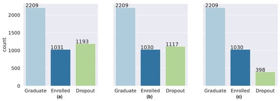
Figure 1.
Distribution of the records among the three defined labels and for the datasets built with: (a) information at the time of enrollment (S0); (b) information at the end of first academic semester (S1); (c) information at the end of second academic semester (S2).
The lower number of samples with the label “Dropout” in dataset S2 is due to the fact that once the student drops out, those records are removed from the academic system. Although the entries regarding these students could be kept in the datasets, we opted to remove them because the final goal is to develop a system that can be used in the real scenario, where students’ records are removed once they drop out. It is also worth noticing that most students who drop out do it during the second semester.
Figure 1 shows that for datasets S0 and S1, there is one majority class (“Graduate”) with half the number of total records and two equally distributed minority classes with approximately a quarter of the records each. However, for dataset S2, the two minority classes differ significantly from each other, with the label “Dropout” being the less represented class with only 10% of the registers.
The most important classes for accurate classification are the minority ones since the students from these classes are the ones that might benefit the most from planned interventions for academic support and guidance. At the same time, the imbalanced nature of the data poses additional challenges to the machine learning models. Therefore, the machine learning algorithms used were selected based on their ability to deal with a multi-class classification problem with imbalanced data, as previously explained.
4.3. Machine Learning Models
Based on previous works with a similar dataset from the same institution [33], the chosen reference method for building classification models for the three-time phases used was SMOTE as a re-sampling strategy for the imbalanced classes, followed by the use of Random Forest to build the classification models (SMOTE + RF). Two other methods were used that deal with the imbalanced nature of data: SVMSMOTE, followed by Random Forest (SVMSMOTE + RF) and the RusBoost algorithm (RB). Additionally, two algorithms that incorporate the strategies to deal with imbalanced datasets were used. These are the Balanced Random Forest classifier (BRF) and the Easy Ensemble classifier (EE). Therefore, fifteen different models were built, five for each of the datasets representing the data in the three different moments.
Following the usual procedure, the datasets were divided into training (90% of total records) and test sets, including a stratification procedure to ensure that the original proportion of the samples in each class was preserved in each set. In the case of SMOTE + RF, the SMOTE algorithm was applied to the training datasets. For all the datasets, a 10-fold cross-validation approach was used for model training, meaning that the training dataset was divided into 10 blocks, and the training of each model was conducted with 9 of the blocks, with the remaining one being used for validation purposes. The process was repeated 10 times, once for each block, thus enabling the maximization of the total number of observations used for validation while avoiding over-fitting. The cross-validation procedure also included the class stratification procedure. The test sets, kept aside until this point, were used for validation of the models.
4.4. Model Evaluation and Feature Importance
To assess model performance, the balanced accuracy and the global F1 score were used, which are adequate metrics for models built with imbalanced datasets [23]. F1 score is the harmonic mean between precision and recall and is computed according to the following equation:
where TP is the number of true positives, FP is the number of false positives, and FN is the number of true negatives.
Accuracy is the fraction of correct predictions out of the total number of predictions and is computed according to Equation (2),
where TN is the number of true negatives.
Moreover, since it is important to understand the models’ behavior for each class, the individual F1 scores were also analyzed. The confusion matrices, which provide more detailed information regarding miss-classification for each class, were also obtained and analyzed.
Data splitting and model training were repeated 10 times with different random number generator seeds, both for the train-test split procedure and for the cross-validation and classifier. This allowed for checking the dependency to the randomness of each model. The overall estimates of the evaluation metrics were obtained by the average values and respective standard deviation values across the 10 runs of the procedure.
To better understand how the learners perform the classification tasks, the feature importance for the best three models, built with each dataset, were computed. These computations are easily performed for the Random Forest based models since they are provided by one of the attributes of the model’s object. In such cases, the feature importance is computed as the total reduction of the criterion (the Gini impurity index) brought by that feature on average over all the trees in the forest.
4.5. Software and Equipment
Several dedicated Python libraries were used to develop this work, namely, pandas [34] for data analysis and data wrangling, seaborn [35] for data visualization, scikit-learn [36] for general machine learning tasks, and the imbalanced-learn [37] module for data balancing algorithms. All the computations ran on the Ubuntu operating system on an NVIDIA DGX Station computer with 2 CPU Intel Xeon E5-2698V4 with 20 core 2.2 GHz, 256 GB of memory, and 4 NVIDIA Tesla V100 GPU.
5. Results and Discussion
The global evaluation metrics for each model and for each dataset are presented in Table 3 (dataset at the time of enrollment, S0), Table 4 (dataset at the end of the first semester, S1), and Table 5 (dataset at the end of the second semester, S2). The metrics presented are the global F1 score for the train and test sets and also the balanced accuracy for the test set.
Table 3.
Global evaluation metrics for each learning model built with the information at the time of enrollment (dataset S0). Values represent mean and standard deviation.
Table 4.
Global evaluation metrics for each learning model built with the information at the end of first semester (dataset S1). Values represent mean and standard deviation.
Table 5.
Global evaluation metrics for each learning model built with the information at the end of second semester (dataset S2). Values represent mean and standard deviation.
Globally, there is a significant improvement on the models from S0, where the best F1 score is 0.650, to S1, where the best F1 score is 0.745. This was expected because dataset S0 lacked information regarding academic results after enrollment. On the other hand, dataset S1 already included some information concerning how the student was academically reacting to higher education. Such metrics’ improvement is not as sharp when models for S2 are analyzed. For S2, the best F1 score is 0.741, a very similar value to the best F1 score for S1. Although dataset S2 included additional academic performance information, it also had a more sharp imbalanced distribution of registers among the classes, which poses extra constraints to the machine learning algorithms.
The models that tackle class imbalance at the data level present a higher difference between train and test F1 score. This has to do with the nature of the SMOTE and SMOTE-based algorithms. For balancing the datasets, SMOTE-based algorithms add synthetic examples to the minority classes at the training stage. However, at the test stage, they are applied to inherently imbalanced datasets. On the other hand, class imbalance tackled at the algorithm level does not imply a change in the distribution of the dataset, which naturally results in evaluation metrics’ values similar both for training and testing.
Finally, models SMOTE + RF, SVMSMOTE + RF, and BRF present better results than EE or RB. This holds true for every phase considered.
Besides analyzing global metrics, it is also relevant to analyze models’ performance for each class label. Table 6, Table 7, and Table 8 present F1 scores for each class, for each model, and for datasets S0, S1, and S2, respectively.
Table 6.
F1 score evaluation for each class for each learning model built with information at the time of enrollment. Values represent mean and standard deviation.
Table 7.
F1 score evaluation for each class for each learning model built with information at the end of first semester. Values represent mean and standard deviation.
Table 8.
F1 score evaluation for each class for each learning model built with information at the end of second semester. Values represent mean and standard deviation.
The F1 scores for the class “Graduate”, the most populated one, are consistently higher than scores for the other two classes. The next highest scores correspond to the second most populated class in each dataset: “Dropout” in the case of dataset S1 and “Enrolled” in the case of dataset S2.
The highest scores for class “Graduate” are obtained with SVMSMOTE + RF for every phase considered. However, for S0 and S1, the highest scores for the “Enrolled” and for the “Dropout” classes are obtained by BRF. Therefore, if the goal is to obtain a most accurate prediction for such classes, Balanced Random Forest models is preferred.
The lowest F1 scores in the entire experiment are obtained for the “Dropout” class at the end of the second semester. This is related to the small number of records labeled “Dropout” in the dataset S2 (only 398 in the whole dataset, of which 358 are used in the training set and 40 in the test set).
The confusion matrices obtained for each dataset, and for each model, are presented in Figure 2, Figure 3 and Figure 4.
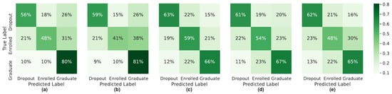
Figure 2.
Confusion Matrices for the models built with dataset S0: (a) SMOTE + RF, (b) SVMSMOTE + RF, (c) BRF, (d) EE, and (e) RB.
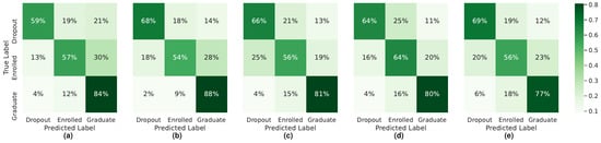
Figure 3.
Confusion Matrices for the models built with dataset S1: (a) SMOTE + RF, (b) SVMSMOTE + RF, (c) BRF, (d) EE, and (e) RB.
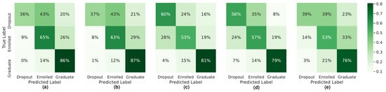
Figure 4.
Confusion Matrices for the models built with dataset S2: (a) SMOTE + RF, (b) SVMSMOTE + RF, (c) BRF, (d) EE, and (e) RB.
Given the small number of students labeled as “Dropout” remaining in dataset S2, as well as the corresponding poor scores, the question is raised whether it would not be better to model the problem for this dataset as a binary one. With this question in mind, an additional experiment was carried out with dataset S2, where registers labeled as “Enrolled” and “Dropout” were relabeled as “Not Graduate”. The data processing, model training, and evaluation for the two-class classification task proceeded as previously described. The results are presented in Table 9.
Table 9.
F1 score evaluation (global and individual) for each learning model built with information at the end of second semester with two classes. Values represent mean and standard deviation.
For the binary classification on dataset S2, the best results are obtained with Balanced Random Forest. F1 score for “Graduate” class is higher than the best value obtained with the three class approach (0.871 ± 0.018 for BRF with the binary approach vs. 0.852 ± 0.005 for SVMSMOTE + RF for the three class approach). The F1 score for the “Not Graduate” class is also significantly higher (0.808 ± 0.026) than the best F1 score values obtained for the “Enrolled” or “Dropout” classes ( 0.616 ± 0.009 and 0.493 ± 0.055, respectively).
Regarding feature importance, Figure 5, Figure 6, and Figure 7 present the relative weights of the top five most important features for the three models with best scores (SMOTE + RF, SVMSMOTE + RF and BRF) for each dataset, S0, S1, and S2, respectively.
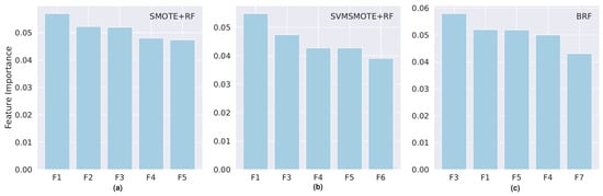
Figure 5.
Top five most important features for models built with dataset S0 for the models with best scores: (a) SMOTE and Random Forest; (b) SVMSMOTE and Random Forest; (c) Balanced Random Forest. F1: Age at enrollment; F2: Tuition fees up to date; F3: Admission Grade; F4: Previous Habilitation Grade; F5: Displaced Student; F6: Degree; F7: Student’s Average Grade at National Exams.
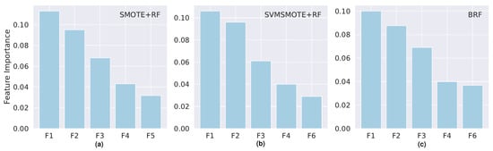
Figure 6.
Top five most important features for models built with dataset S1 for the models with best scores: (a) SMOTE and Random Forest; (b) SVMSMOTE and Random Forest; (c) Balanced Random Forest. F1: Number of CUs approved (1st sem.); F2: Average Grade (1st sem); F3: Number of CU attended (1st sem); F4: Age at enrollment; F5: Tuition fees up to date; F6: Admission Grade.
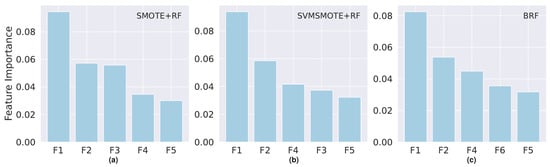
Figure 7.
Top five most important features for models built with dataset S1 for the models with best scores: (a) SMOTE and Random Forest; (b) SVMSMOTE and Random Forest; (c) Balanced Random Forest. F1: Number of CUs approved (second sem.); F2: Number of CUs approved (first sem.); F3: Tuition fees up to date; F4: Average Grade (second sem); F5: Age at enrollment; F6: Average Grade (first sem).
The most important features vary greatly among the different datasets and only mildly between the models for the same dataset. For dataset S0, the features that belong to the top five and that are common to the three models are “Age at enrollment”, “Admission Grade”, “Previous Habilitation Grade”, and “Displaced Student”. The “Degree”, “Average Grade at the National Exams” and “Tuition fees up to date” are on the top five list for at least one of the models. The weights of the feature importance are similarly low in all of the cases and close to 0.05.
In the case of dataset S1, the three most important features common to all the models refer to the academic performance after the enrollment: “Number of CUs approved (first sem)”, the “Average Grade (first sem)”, and the “Number of CU attended (first sem)”. The “Age at enrollment”, “Tuition fees up to date”, and the “Admission Grade” features also belong to the top five of at least one of the models, although with lower relative scores.
In the case of dataset S2, the features related to the academic performance are also the most important: “Number of CUs approved” in the second and in the first semester and the “Average Grade” in the second semester.
Overall, the features related to the macroeconomic situation, the social-economic features, and the demographic features are of irrelevant importance in the models, at the detriment of features related to the academic performance after enrollment. This holds true only for the datasets S1 and S2 since S0 does not contain such information. The “Age at enrollment” is the only social–demographic feature that consistently appears in the top five list of feature importance. Worthy of note is the fact that for datasets S0 and S2, all the features present low feature importance scores, below 0.10. The maximum feature importance score is slightly above 0.10 for the most important feature in dataset S2.
The results obtained compare fairly with some other works that attempt to predict students’ dropout or academic performance at early stages, although our performance results are slightly lower. For instance, in a study to predict dropout at early stages [16], the authors obtained a model with 72% accuracy at the time of enrollment and 82% by the end of the first semester. A dataset from an engineering school was used. In another study for performance prediction [10], the model achieved 79% accuracy for the prediction of students’ performance at the time of admission in a Computer Science degree. Both works used datasets from specific fields of study and binary classification tasks. This is in contrast with our multi-class problem using a heterogeneous dataset, which includes samples from several different fields of study and different schools, and it might explain the slightly lower performance scores of our models.
6. Final Remarks
The primary objective of this research was to develop machine learning models that can contribute to the early detection of students at risk of dropping out or not finishing their degree in due time. Three different versions of a base dataset were built comprising social–demographic, macroeconomic, and academic information at different time phases along the first academic year of the students. Five machine learning algorithms were used to train prediction models at each phase.
The obtained results show that it is possible to obtain reasonable classifiers and that the best models are based on decision trees, either using data level methods (SMOTE, SVMSMOTE) or algorithm data level (Balanced Random Forest) to deal with the imbalanced nature of the data. Results also show that the best moment for early prediction is by the end of the first semester, when information regarding academic performance after enrollment is already available.
The models are now incorporated in a proprietary Learning Analytics platform and are being applied to the students enrolled for the first time in the higher education institution. The information provided by the models is being used as an auxiliary tool to select incoming students to participate as mentees in the mentoring activities of the higher education institution.
It is foreseen that the models are updated yearly and validated either with the new information of incoming students or with the information of the final situation of the already enrolled students.
This study exhibits certain limitations that pave the way for future lines of research. For instance, this work does not consider the specific characteristics of the different courses and different schools of the polytechnic university under study. A future line of research is the investigation of different prediction models for the different schools and courses in order to further improve the early prediction results. The imbalanced nature of the dataset is another limitation of this work. Although we used strategies to deal with it, the developed models still perform better on the majority class. Therefore, a possible future line of research is the investigation of the use of a one-class classification approach to improve models’ performance [38]. Finally, our study does not consider the information regarding the interaction of the students with the learning management platform. This is an active field of research, which has already shown to provide good results in classification tasks [19,39]. In the future, we plan to include this information in our datasets and to investigate its impact in the performance of the models. Along this line of research, it would also be interesting to take into account the relevant cognitive functions and personality traits of the students [40,41].
Author Contributions
Conceptualization, M.V.M., J.M., L.B. and V.R.; methodology, M.V.M., J.M. and V.R.; software, M.V.M.; validation, J.M. and L.B.; data curation, V.R. and J.M.; visualization, M.V.M.; writing—original draft preparation, M.V.M.; writing—review and editing, L.B.; project administration, V.R.; funding acquisition, V.R. All authors have read and agreed to the published version of the manuscript.
Funding
This research was funded by program SATDAP—Capacitação da Administração Pública 388 under grant number POCI-05-5762-FSE-000191 and by national funds through the Fundação para a Ciência e a Tecnologia, I.P. (Portuguese Foundation for Science and Technology) by the project UIDB/05064/2020 (VALORIZA—Research Centre for Endogenous Resource Valorization).
Institutional Review Board Statement
Privacy issues related to the use and publication of the dataset were validated by the Data Protection Officer (DPO) of the Polytechnic Institute of Portalegre according to the General Data Protection Regulation (GDPR) directives.
Informed Consent Statement
Not applicable.
Data Availability Statement
A version of the dataset generated during the study is publicly available at https://zenodo.org/record/5777340 (accessed on 11 January 2022) under Creative Commons Attribution 4.0 International.
Conflicts of Interest
The authors declare no conflict of interest.
Abbreviations
The following abbreviations are used in this manuscript:
| BRF | Balanced Random Forest |
| EE | Easy Ensemble |
| GDPR | General Data Protection Regulation |
| IPP | Polytechnic Institute of Portalegre |
| ML | Machine Learning |
| RF | Random Forest |
| RB | RUSBoost Algorithm |
| RUS | Random Under-Sampling |
| SMOTE | Synthetic Minority Over-sampling Technique |
| SVM | Support Vector Machine |
References
- Cvetkovski, S.; Jorm, A.F.; Mackinnon, A.J. Student psychological distress and degree dropout or completion: A discrete-time, competing risks survival analysis. High. Educ. Res. Dev. 2018, 37, 484–498. [Google Scholar] [CrossRef]
- Byrom, T.; Lightfoot, N. Interrupted trajectories: The impact of academic failure on the social mobility of working-class students. Br. J. Sociol. Educ. 2013, 34, 812–828. [Google Scholar] [CrossRef]
- Rastrollo-Guerrero, J.L.; Gómez-Pulido, J.A.; Durán-Domínguez, A. Analyzing and predicting students’ performance by means of machine learning: A review. Appl. Sci. 2020, 10, 1042. [Google Scholar] [CrossRef]
- Alyahyan, E.; Düştegör, D. Predicting academic success in higher education: Literature review and best practices. Int. J. Educ. Technol. High. Educ. 2020, 17, 3. [Google Scholar] [CrossRef]
- Miguéis, V.L.; Freitas, A.; Garcia, P.J.; Silva, A. Early segmentation of students according to their academic performance: A predictive modelling approach. Decis. Support Syst. 2018, 115, 36–51. [Google Scholar] [CrossRef]
- Helal, S.; Li, J.; Liu, L.; Ebrahimie, E.; Dawson, S.; Murray, D.J.; Long, Q. Predicting academic performance by considering student heterogeneity. Knowl.-Based Syst. 2018, 161, 134–146. [Google Scholar] [CrossRef]
- Dien, T.T.; Luu, S.H.; Thanh-Hai, N.; Thai-Nghe, N. Deep learning with data transformation and factor analysis for student performance prediction. Int. J. Adv. Comput. Sci. Appl. 2020, 11, 711–721. [Google Scholar] [CrossRef]
- Wakelam, E.; Jefferies, A.; Davey, N.; Sun, Y. The potential for student performance prediction in small cohorts with minimal available attributes. Br. J. Educ. Technol. 2020, 51, 347–370. [Google Scholar] [CrossRef]
- Ghorbani, R.; Ghousi, R. Comparing Different Resampling Methods in Predicting Students’ Performance Using Machine Learning Techniques. IEEE Access 2020, 8, 67899–67911. [Google Scholar] [CrossRef]
- Mengash, H.A. Using data mining techniques to predict student performance to support decision making in university admission systems. IEEE Access 2020, 8, 55462–55470. [Google Scholar] [CrossRef]
- Yağcı, M. Educational data mining: Prediction of students’ academic performance using machine learning algorithms. Smart Learn. Environ. 2022, 9, 11. [Google Scholar] [CrossRef]
- Hutagaol, N.S. Predictive modelling of student dropout using ensemble classifier method in higher education. Adv. Sci. Technol. Eng. Syst. 2019, 4, 206–211. [Google Scholar] [CrossRef]
- Kemper, L.; Vorhoff, G.; Wigger, B.U. Predicting student dropout: A machine learning approach. Eur. J. High. Educ. 2020, 10, 28–47. [Google Scholar] [CrossRef]
- Kabathova, J.; Drlik, M. Towards predicting student’s dropout in university courses using different machine learning techniques. Appl. Sci. 2021, 11, 3130. [Google Scholar] [CrossRef]
- Bottcher, A.; Thurner, V.; Hafner, T.; Hertle, J. A data science-based approach for identifying counseling needs in first-year students. In Proceedings of the IEEE Global Engineering Education Conference, EDUCON, Vienna, Austria, 21–23 April 2021; pp. 420–429. [Google Scholar] [CrossRef]
- Fernandez-Garcia, A.J.; Preciado, J.C.; Melchor, F.; Rodriguez-Echeverria, R.; Conejero, J.M.; Sanchez-Figueroa, F. A real-life machine learning experience for predicting university dropout at different stages using academic data. IEEE Access 2021, 9, 133076–133090. [Google Scholar] [CrossRef]
- Iatrellis, O.; Savvas, I.; Fitsilis, P.; Gerogiannis, V.C. A two-phase machine learning approach for predicting student outcomes. Educ. Inf. Technol. 2021, 26, 69–88. [Google Scholar] [CrossRef]
- Chen, Y.; Zheng, Q.; Ji, S.; Tian, F.; Zhu, H.; Liu, M. Identifying at-risk students based on the phased prediction model. Knowl. Inf. Syst. 2020, 62, 987–1003. [Google Scholar] [CrossRef]
- Qiu, F.; Zhang, G.; Sheng, X.; Jiang, L.; Zhu, L.; Xiang, Q.; Bo, J.; Chen, P.K. Predicting students’ performance in e-learning using learning process and behaviour data. Sci. Rep. 2022, 12, 453. [Google Scholar] [CrossRef]
- Lagus, J.; Longi, K.; Klami, A.; Hellas, A. Transfer-Learning Methods in Programming Course Outcome Prediction. ACM Trans. Comput. Educ. 2018, 4, 1–18. [Google Scholar] [CrossRef]
- Nagy, M.; Molontay, R. Predicting Dropout in Higher Education Based on Secondary School Performance. In Proceedings of the INES 2018—IEEE 22nd International Conference on Intelligent Engineering Systems, Las Palmas de Gran Canaria, Spain, 21–23 June 2018; pp. 000389–000394. [Google Scholar] [CrossRef]
- Beaulac, C.; Rosenthal, J.S. Predicting University Students’ Academic Success and Major Using Random Forests. Res. High. Educ. 2019, 60, 1048–1064. [Google Scholar] [CrossRef]
- Tanha, J.; Abdi, Y.; Samadi, N.; Razzaghi, N.; Asadpour, M. Boosting methods for multi-class imbalanced data classification: An experimental review. J. Big Data 2020, 7, 70. [Google Scholar] [CrossRef]
- Ali, A.; Shamsuddin, S.M.; Ralescu, A.L. Classification with class imbalance problem: A review. Int. J. Adv. Soft Comput. Its Appl. 2015, 7, 176–204. [Google Scholar]
- Chawla, N.V.; Bowyer, K.W.; Hall, L.O.; Kegelmeyer, W.P. SMOTE: Synthetic minority over-sampling technique. J. Artif. Intell. Res. 2002, 16, 321–357. [Google Scholar] [CrossRef]
- Nguyen, H.M.; Cooper, E.W.; Kamei, K. Borderline over-sampling for imbalanced data classification. Int. J. Knowl. Eng. Soft Data Paradig. 2011, 3, 4. [Google Scholar] [CrossRef]
- Seiffert, C.; Khoshgoftaar, T.M.; Van Hulse, J.; Napolitano, A. RUSBoost: A hybrid approach to alleviating class imbalance. IEEE Trans. Syst. Man Cybern. Part A Systems Humans 2010, 40, 185–197. [Google Scholar] [CrossRef]
- Freund, Y.; Schapire, R.E. A decision-theoretic generalization of on-line learning and an application to boosting. Lect. Notes Comput. Sci. 1995, 904, 23–37. [Google Scholar] [CrossRef]
- Breiman, L. Random forests. Mach. Learn. 2001, 45, 5–32. [Google Scholar] [CrossRef]
- Quinlan, J.R. Induction of decision trees. Mach. Learn. 1986, 1, 81–106. [Google Scholar] [CrossRef]
- Chen, C.; Liaw, A.; Breiman, L. Using Random Forest to Learn Imbalanced Data; Technical Report; University of California: Berkeley, CA, USA, 2004. [Google Scholar]
- Liu, X.Y.; Wu, J.; Zhou, Z.H. Exploratory undersampling for class-imbalance learning. IEEE Trans. Syst. Man Cybern. Part Cybern. 2009, 39, 539–550. [Google Scholar] [CrossRef]
- Martins, M.V.; Tolledo, D.; Machado, J.; Baptista, L.M.; Realinho, V. Early Prediction of Student’s Performance in Higher Education: A Case Study; Springer International Publishing: Cham, Switzerland, 2021; Volume 1365, pp. 166–175. [Google Scholar] [CrossRef]
- McKinney, W. Data Structures for Statistical Computing in Python. In Proceedings of the 9th Python in Science Conference, Austin, TX, USA, 28 June–3 July 2010; pp. 56–61. [Google Scholar] [CrossRef]
- Waskom, M.L. Seaborn: Statistical data visualization. J. Open Source Softw. 2021, 6, 3021. [Google Scholar] [CrossRef]
- Pedregosa, F.; Varoquaux, G.; Gramfort, A.; Michel, V.; Thirion, B.; Grisel, O.; Blondel, M.; Prettenhofer, P.; Weiss, R.; Dubourg, V.; et al. Scikit-learn: Machine learning in Python. J. Mach. Learn. Res. 2011, 12, 2825–2830. [Google Scholar]
- Lemaître, G.; Nogueira, F.; Aridas, C. Imbalanced-learn: A python toolbox to tackle the curse of imbalanced datasets in machine learning. J. Mach. Learn. Res. 2017, 18, 559–563. [Google Scholar]
- Seliya, N.; Zadeh, A.A.; Khoshgoftaar, T.M. A literature review on one-class classification and its potential applications in big data. J. Big Data 2021, 8, 122. [Google Scholar] [CrossRef]
- Zhao, L.; Chen, K.; Song, J.; Zhu, X.; Sun, J.; Caulfield, B.; Mac Namee, B. Academic performance prediction based on multisource, multifeature behavioral data. IEEE Access 2021, 9, 5453–5465. [Google Scholar] [CrossRef]
- Gallego, M.G.; Perez de los Cobos, A.P.; Gallego, J.C.G. Identifying Students at Risk to Academic Dropout in Higher Education. Educ. Sci. 2021, 11, 427. [Google Scholar] [CrossRef]
- Sultana, S.; Khan, S.; Abbas, M. Predicting performance of electrical engineering students using cognitive and non-cognitive features for identification of potential dropouts. Int. J. Electr. Eng. Educ. 2017, 54, 105–118. [Google Scholar] [CrossRef]


Disclaimer/Publisher’s Note: The statements, opinions and data contained in all publications are solely those of the individual author(s) and contributor(s) and not of MDPI and/or the editor(s). MDPI and/or the editor(s) disclaim responsibility for any injury to people or property resulting from any ideas, methods, instructions or products referred to in the content. |
© 2023 by the authors. Licensee MDPI, Basel, Switzerland. This article is an open access article distributed under the terms and conditions of the Creative Commons Attribution (CC BY) license (https://creativecommons.org/licenses/by/4.0/).