Influence of Hyperparameters in Deep Learning Models for Coffee Rust Detection

Abstract

Most of the world’s crops can be attacked by various diseases or pests, affecting their quality and productivity. In recent years, transfer learning with deep learning (DL) models has been used to detect diseases in maize, tomato, rice, and other crops. In the specific case of coffee, some recent works have used fixed hyperparameters to fine-tune the pre-trained models with the new dataset and/or applied data augmentation, such as image patching, to improve classifier performance. However, a detailed evaluation of the impact of architecture (e.g., backbone) and training (e.g., optimizer and learning rate) hyperparameters on the performance of coffee rust classification models has not been performed. Therefore, this paper presents a comprehensive study of the impact of five types of hyperparameters on the performance of coffee rust classification models. Specifically, eight pre-trained models are compared, each with four different amounts of transferred layers and three different numbers of neurons in the fully-connected (FC) layer, and the models are fine-tuned with three types of optimizers, each with three learning rate values. Comparing more than 800 models in terms of F1-score and accuracy, it is identified that the type of backbone is the hyperparameter with the greatest impact (with differences between models of up to 70%), followed by the optimizer (with differences of up to 20%). At the end of the study, specific recommendations are made on the values of the most suitable hyperparameters for the identification of this type of disease in coffee crops.

1. Introduction

Plant pests and diseases are one of the major problems affecting food security worldwide [1]. Due to the impact of climate change on the incidence of pests and diseases, actions for their protection, e.g., crop monitoring, are mandatory [2]. However, this is a time-consuming and costly task for the farmer [3]. Within the technological solutions for crop monitoring, artificial intelligence (AI) and deep learning (DL) techniques have demonstrated high accuracy values in the detection of pests and diseases [4]. However, challenges remain when using these types of models in natural environments (e.g., variability of colors, shapes, textures, and light) [5], while the number of examples in the image sets used to train these models has not been very large. In turn, their images may contain distractors (e.g., the hand or shoes of the farmer), which could divert the attention of the model into false patterns that affect the decision about the presence of the disease in the plant [6,7].

In the state-of-the-art, there are numerous solutions for crop disease identification using transfer learning with DL-based models. For example, a GoogLeNet-based model allows the identification of 38 classes of 14 crop species and 26 diseases, under controlled conditions using the Plantvillage dataset (54,303 images) [8]; the model achieved 99.25% accuracy using weight transfer, and 98.24% accuracy with fine-tuning. However, when the trained model was evaluated with a different dataset, the accuracy was reduced to 31%. Although these differences between the training/validation set and the test set may be related to overfitting, they may also be due to the test set being more complex than the training/validation set, or to the fact that the test set is not necessarily more complex but simply different than the training/validation set [9]. Similarly, a pre-trained network based on GoogLeNet was used to classify leaf diseases of 12 plant species (56 classes in total). In that study, the usefulness of a small dataset (i.e., 1383 images) was evaluated, reaching accuracy values for the classes between 65% and 100% [10]. Likewise, the trained model was evaluated with images of the dataset after background removal, obtaining better accuracy values for most of the classes [11]. In another study, a combination of CNN (Convolutional Neural Networks) architectures (specifically VGG16 + Inception) was used for the classification of maize and rice diseases from the Plantvillage dataset (3852 images, 4 categories), and the accuracy obtained was 92% for rice and 80% for maize. Additionally, this hybrid model was compared against other models obtained by transfer learning, whose accuracy results were 65.19% for VGG19, 85.56% for Inceptionv3, 65.19% for ResNet50 and 80.27% for DenseNet [12].

Specifically in coffee leaf monitoring, several pre-trained models (e.g., AlexNet, GoogLeNet, VGG16, ResNet50 and MobileNetV2) have been used for disease identification [13,14]. For instance, DL-based models were trained with a dataset of Arabica coffee leaves affected by 4 types of diseases and 5 levels of affectation (healthy, very low 0.1–5%, low 5.1–10%, high 10.1–15% and very high >15%), obtaining accuracy results between 90% and 95%. However, the authors warn of the need to use images captured in real environments, as they differ from images of controlled environments, for example, in terms of illumination and the presence of shadows [10]. In another study, ResNet was used as the backbone of the model, and two types of datasets were used to train and validate it. The first one corresponds to raw images from the RoCoLe dataset, and the second one corresponds to a mixture between binary segmentation and patches of the original images. According to the results, the model trained with the second dataset provides an accuracy of 98% versus 75% of the model trained with the first dataset [15].

The solutions proposed in the literature for the classification of coffee leaf diseases (Rust, Phoma, Cercospora, Leaf Miner an others) have used a diversity of hyperparameters that do not facilitate specific conclusions. In the case of the optimizer, SGD [14,16,17,18], Adam [18,19], or RMSprop [18] have been used, both with fixed learning rates ([0.01, 0.001] [17,20]) and learning rate values selected from a range ([0.001–0.3], [0.01–0.00001] [14,18]). The number of units in the fully connected layer, prior to the classification layer, was also implemented with values in the range 20–200 [14], or 256–1024 [21]. Dropouts of 0.5 [18], or 0.8 [19] have also been applied. These models have been trained from 20 to 300 epochs [16,17,19,20,21], with batch sizes including 16, 32 or 64 images [17,19,21]. Regarding the architecture types, models with specific design [17] and models by transfer learning have been evaluated, including MobileNetV2 [19], DenseNet [19], InceptionResNetV2 [19], ALexNet [20], GoogLeNet [17], VGG16 [21], ResNet50 [16,17,19], and Xception [21]. Also, fine tuning [18] or data augmentation [21] have been involved.

In summary, the state-of-the-art works have assumed the values of hyperparameters for both architecture (e.g., network type, network depth, neurons in fully connected layers) and training (e.g., optimizer, learning rate), but have not performed an exhaustive evaluation of their impact on model performance. Neither have they proposed a concrete methodology to rank the hyperparameters and make decisions on their values for the in-crop disease detection problem. For this reason, this study proposes a model-centered methodology for image classification tasks (specifically crop disease detection) that allows answering the following questions: what types of hyperparameters are the most influential on the classifier performance? and how to organize an experiment that allows selecting the best values of these hyperparameters?

The main contributions of this study include the following results:

• We propose a methodology for model-centric deep learning projects that allows hierarchization of hyperparameters and selection of the most appropriate values for the performance of crop disease detection models.
• This methodology was applied to the problem of rust detection in coffee crops and allowed to rank five types of hyperparameters (type of network, depth, number of neurons in the FC layer, optimizer and learning rate), as well as to identify values that allow to improve classifier performance.
• With this methodology, it was possible to improve the F1-score of the classifier from 18.4% to 92.71%, without making any adjustments to the image set.

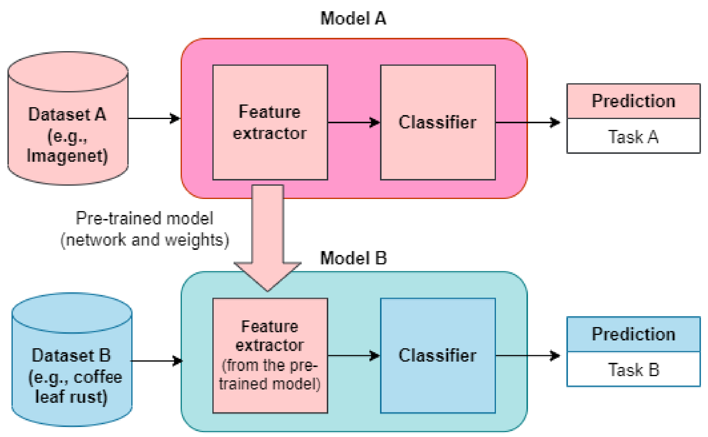
The remainder of the study is organized as follows. Section 2 explains preliminary concepts related to convolutional neural networks (CNN) and transfer learning. Section 3 is focused on the materials and methods of the current study, specifically the coffee leaf rust dataset and the proposed methodology to identify the hyperparameters with the greatest impact on the performance of coffee rust classification models. Section 4 shows the results of the study, and Section 5 is the discussion of the research. Finally, Section 6 concludes the study.

2. Preliminary Concepts

This section explains some concepts associated with CNNs and transfer learning.

2.1. Convolutional Neural Networks

In general, an artificial neural network is constructed from the weighted sum of many simple functions (each executed by a single neuron), whose output feeds a nonlinear function or activation function (e.g., ReLU). The function of each neuron is determined by adjustable parameters, which can be iteratively updated (from initial values and examples of inputs and outputs) until the trainable function performs the desired task. The training process refers to the adjustment of the parameters (e.g., weights and biases) that relate the units of the network in order to reduce the error between the actual value and the value predicted by the model. Based on this concept, recent models have been developed such as CNN, recurrent neural networks, and transformers that allow pattern recognition in images, text, speech, or video.

Convolutional neural networks are a type of neural network that allow the extraction of features in images without the need to elaborate complex rules; consequently, they have been mainly used in computer vision applications for object classification and detection tasks in images. They are mainly composed of convolutional layers, pooling layers, and dense layers [22]. Convolutional layers are the main component of these models, which involve a set of spatial filters that apply a cross-correlation operation on a neighborhood. The pooling layers are used to synthesize the information in each neighborhood, either by calculating the average value (average pooling) or by extracting the maximum value (max pooling). In addition, there are layers that operate on the entire input feature map, either through a global pooling operation that extracts a single value or through the use of dense layers or fully connected (FC) layers that are usually applied at the end of the network for classification purposes [23].

In addition, hyperparameters are those values that are not learned by the model but adjusted by the designer in relation to the architecture (e.g., type of architecture, network depth, number of filters or neurons), or the training (e.g., type of optimizer, learning rate, number of epochs, batch size) [24].

In terms of architecture, there are different typologies of CNN. Sequential networks (e.g., VGG11, VGG16, and VGG19) have different depths based on sequential blocks and pooling layers [25]. Residual networks (e.g., ResNet50, ResNet101, ResNet152) use additional connections between convolutional layers of different depth levels [26]. Parallel networks (e.g, InceptionV3) use concatenation connections between convolutional layers of the same depth level [27]. InceptionResNet is a combination of architectures within Inception and ResNet blocks [28]. Separable convolution networks (e.g., MobileNet, Xception) use a depth-wise convolution followed by a point-wise convolution [29,30]. Dense networks exploit the potential of the network by reusing features and connecting layers in a feed-forward manner to ensure maximum information flow between them [31].

Table 1. Information of some pre-trained models for image classification tasks. FC stands for fully connected layer.

Pre-Trained Model	Authors	Default Input Size	No. of Layers (FC Included)	No. of Parameters
VGG19 [25]	(Simonyan, 2014)	$224\times 224$	19	143,667,240
ResNet50 [26]	(He, 2016)	224 × 224	152	25,636,712
InceptionV3 [28]	(Szegedy C. V., 2016)	299 × 299	159	23,851,784
Xception [30]	(Chollet, 2017)	299 × 299	126	22,910,480
MobileNetV2 [32]	(Sandler, 2018)	224 × 224	88	3,538,984
DenseNet201 [31]	(Huang, 2017)	224 × 224	201	20,242,984
EfficientNetB5 [33]	(Tan, 2019)	456 × 456		30,562,527
InceptionResNetV2 [34]	(Szegedy C. I., 2016)	299 × 299	572	55,873,736

presents a summary of the number of parameters and layers of some representative state-of-the-art networks for image classification tasks.

2.2. Transfer Learning

Transfer learning is a design strategy in which information from a pre-trained model for a specific machine learning task is used in a new problem, either with differences in the complexity of the two tasks, or from one model trained with more data to another with less data (using a different dataset) [35,36,37]. At the image classification level, state-of-the-art landmark models were trained with the ImageNet dataset, initially made up of 1 million images with 1000 per class [38]. Furthermore, much of the model is transferred (except at least the classification layer) and retrained with a new set of images, which is typically smaller than ImageNet. The advantage of using transfer learning is that the pre-trained model is able to identify different types of features (e.g., edges, shapes, textures, and colors), due to the great variety of images with which it was pre-trained, allowing the transferred weights require only a small fine-tuning for the new classification task. In Figure 1, a schematic diagram of the transfer learning process is presented, where the pre-trained feature extraction block is used for a new classification task application.

3. Methodology

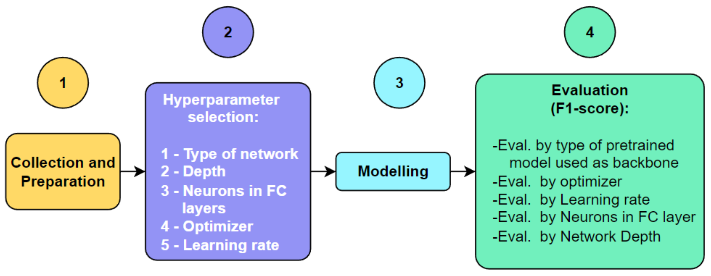
The methodology used in this study is presented in Figure 2. It is mainly composed of four parts: (1) collection and preparation of the dataset; (2) hyperparameter selection; (3) modelling; and (4) evaluation.

Each of the phases of the proposed methodology applied to the detection of coffee leaf rust will be explained below.

3.1. Collection and Preparation of the Dataset

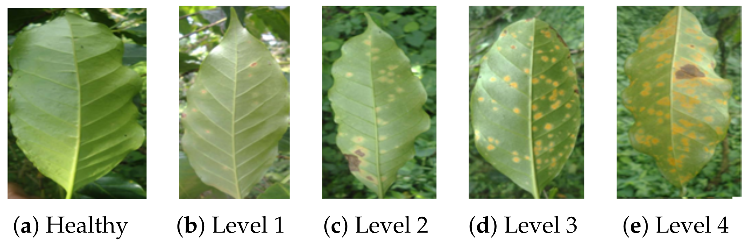
The process of preparing and consolidating the data used in the research was developed in three steps: collection, pre-processing and distribution. First, images were collected from different datasets for coffee leaf rust detection. Specifically, we collected images from: RoCoLe [39], Bracol [40], Digipathos [10], D&P [41], and Licole [21]. The purpose was to have images that vary in background (e.g., natural background or white background), rust severity (see Figure 3), and image brightness.

As a result,

Table 2. Number of images used for coffee leaf rust classification in the present study from state-of-the-art datasets: H (Healthy), R (Rust), and Other.

Dataset	Healthy	Rust	Other
Bracol [40]	272	272	751
RoCoLe [39]	789	602	167
D&P [41]	0	285	257
Digipathos [10]	4	49	139
Licole [21]	621	515	614
Total	1686	1723	1928

summarizes the number of images used from each dataset for the three classes: healthy, rust and other diseases: leaf miner, phoma, cercospora, red spider mite, bacterial blight, blister spots and sooty molds.

Second, several data preparation tasks were applied with the objective of having a clean dataset. For example, distractors in the images that could bias the classification process were removed. More specifically, the tasks focused on:

• Apply crop to have a single leaf per image.
• Remove background that does not belong to the white background or natural environment of the leaf.
• Discard images that contain rust along with other diseases on the same leaf.
• Enlarge the image to fit the coffee leaf.

Finally, the new dataset was divided into training, validation, and testing according to the distribution shown in

Table 3. Summary of the distribution of images in the proposed dataset.

Classes	Training	Validation	Testing
Healthy	1378	146	162
Other	1378	176	202
Rust	1566	159	170
Total	4322	481	534

.

3.2. Hyperparameter Selection

This is the most important phase of a model-centered methodology. First, when selecting the hyperparameters for the study, both architecture and training hyperparameters should be considered. According to state-of-the-art publications, the most commonly used architectural hyperparameters are the type of network, the depth of the network, and the number of neurons in the FC layers. On the other hand, at the level of training hyperparameters, the most used are the optimizer and its learning rate. Second, for each hyperparameter, the number of options and their corresponding values must be defined. At this stage, it is recommended to evaluate at least three options per hyperparameter. In the case of network type, it is common to select pre-trained models of different architecture types, for example, sequential, parallel, residual, and sparse convolutions. For the depth of the net, it is possible to select a shallow layer, a medium depth layer or a deep layer. Regarding the number of neurons in the fully connected layer prior to the classification layer, it typically ranges from 256 to 1024 neurons. In the case of the Optimizer, options such as Adam (or one of its variations), SGD, and RMSprop are usually chosen. Finally, in the case of the Learning Rate, values close to the default values are usually selected in each optimizer, varying them in powers of 10 (positive and negative).

For the search and selection of hyperparameters, a first alternative is to use an algorithm to automatically search the entire space of possible configurations, which is not practical because the space of possible configurations is extremely large. The second alternative is to start with a base configuration and add features based on solid testing, constantly updating a more limited search space. Each round of experiments should have a clear objective and be narrow in order to achieve the goal [42].

Accordingly, the objectives of each round of experiments conducted in this research were assigned as follows: evaluation by pre-trained model used as backbone (for eight pre-trained models), evaluation by the optimizer (between three optimizers), evaluation by the learning rate (LR, using three values), evaluation by the number of neurons in the top FC layer (three values) and evaluation by the network depth (four network depths) (see

Table 4. Stage 2: Hyperparameters and values selected in this study.

Type	Hyperparameter	Number of Options	Values
Architecture	Pre-trained model	8	VGG19, ResNet50, InceptionV3 InceptionResNetV2, MobileNetV2 DenseNet201, EfficientNetB5, Xception
	Network Depth	4	L1 (deeper), L2, L3, L4 (shallower)
	Neurons (FC layer)	3	256, 512 and 1024
Training	Optimizer	3	SGD, Nadam, RMSprop
	Learning Rate (LR)	3	$1\times {10}^{-4}$, $1\times {10}^{-5}$, $1\times {10}^{-6}$

). Although a greater number of options per hyperparameter allows a better selection of its value, it must be taken into account that the number of models to be trained is equal to the multiplication of the options of each hyperparameter. For this study, 864 models were trained.

3.3. Modelling

In this phase, the 864 models were trained with the dataset obtained in the collection and preparation phase. All models were trained with the same number of epochs (i.e., 30) and batch size (i.e., 32). The input images were set to a size of $224\times 224$ pixels.

3.4. Evaluation

Typically, the analysis of the performance of image classification models in balanced problems (with a similar number between classes) is completed by means of a confusion matrix. In short, the confusion matrix is a table that cross-references information about the actual class and the class predicted by the model. From the confusion matrix, it is possible to compute metrics such as accuracy (Equation (1)), precision (P) (Equation (2)), recall (R) (Equation (3)), or F1-score (Equation (4)). These metrics are calculated from the number of correct classifications (TP:True Positives and TN:True Negatives), and the number of incorrect classifications (FP: False Positives and FN: False Negatives).

$$\mathrm{Acc}=\frac{\mathrm{TP}+\mathrm{TN}}{\mathrm{FP}+\mathrm{TP}+\mathrm{TN}+\mathrm{FN}}$$

(1)

$$\mathrm{P}=\frac{\mathrm{TP}}{\mathrm{TP}+\mathrm{FP}}$$

(2)

$$\mathrm{R}=\frac{\mathrm{TP}}{\mathrm{TP}+\mathrm{FN}}$$

(3)

$$\mathrm{F}1=2\frac{\mathrm{P}\times \mathrm{R}}{\mathrm{P}+\mathrm{R}}$$

(4)

For example, for the Healthy class, TP corresponds to correctly classified healthy images, FN corresponds to incorrectly classified Healthy images, TN is correctly classified unhealthy (i.e., rust and other) images, and FP is incorrectly classified unhealthy images. The total result of the metric corresponds to the weighting of the values obtained per class according to the number of images.

All of the above metrics range from 0 to 1, with 0 being the worst performance and 1 being the best. The goal is to select the model with the highest value of the chosen metric, which in this study is the F1-score.

4. Results

According to the purpose of the methodology, we want to determine the importance of the hyperparameter in the performance of the classifier as well as select its best value from the set of defined options. First, the influence of the pre-trained network used as the backbone of the model is evaluated, and then the other hyperparameters grouped by the pre-trained network are assessed.

4.1. Evaluation by Pre-Trained Model Used as Backbone

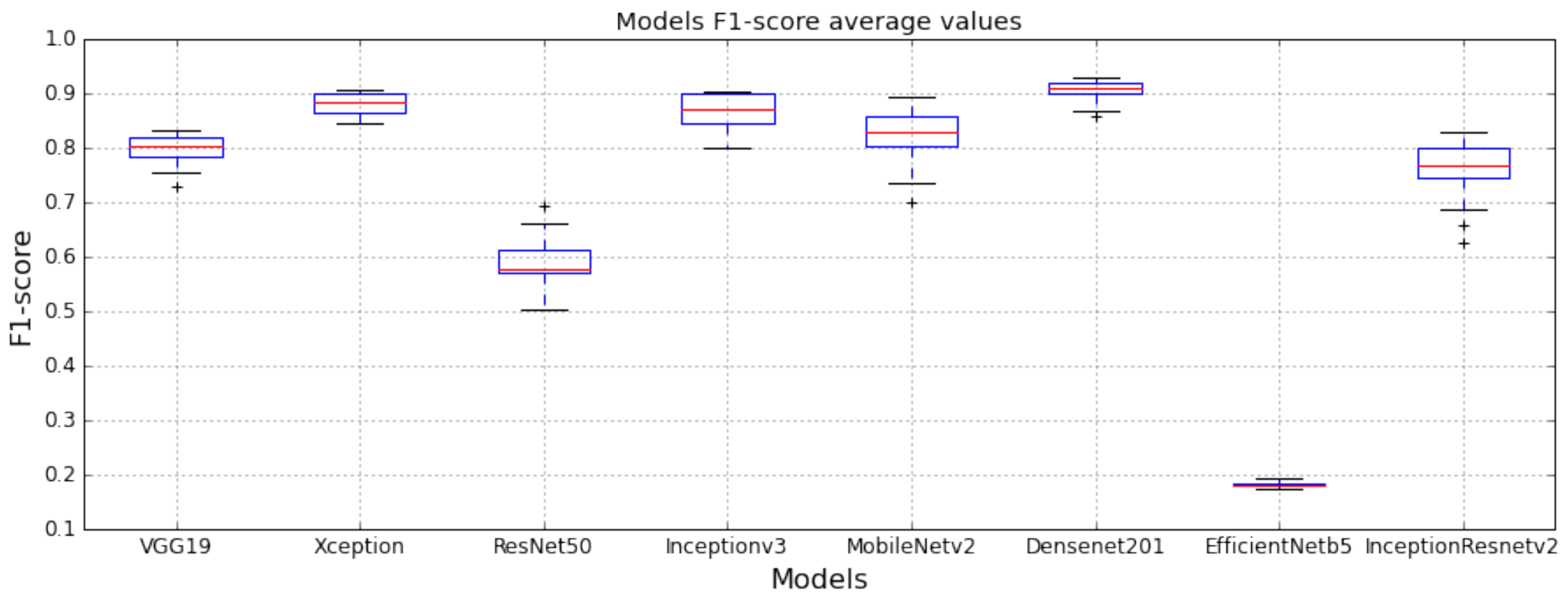
How much does the pre-trained network selected as the backbone influence the F1-score? To answer this question, the 864 models are grouped according to the backbone used, i.e., 108 models per case in this study, and their results are plotted as mean, first, and third quartiles using box plots (see Figure 4).

According to Figure 4, an inappropriate choice of pre-training model will provide F1-score below 20%, while an appropriate choice will provide values above 90%. Specifically, EfficientNetB5 is the least appropriate pre-trained network of the set of options defined in this study, while DenseNet201 is the best option. Other backbones have similar behavior to DenseNet such as: Xception, InceptionV3, MobileNetV2, VGG19, and InceptionResNetV2 (from best to worst). Finally, ResNet50 is not a competitive pre-trained model for this classification problem.

In summary, this hyperparameter has a very high impact on model performance (with variations of up to 70% among them).

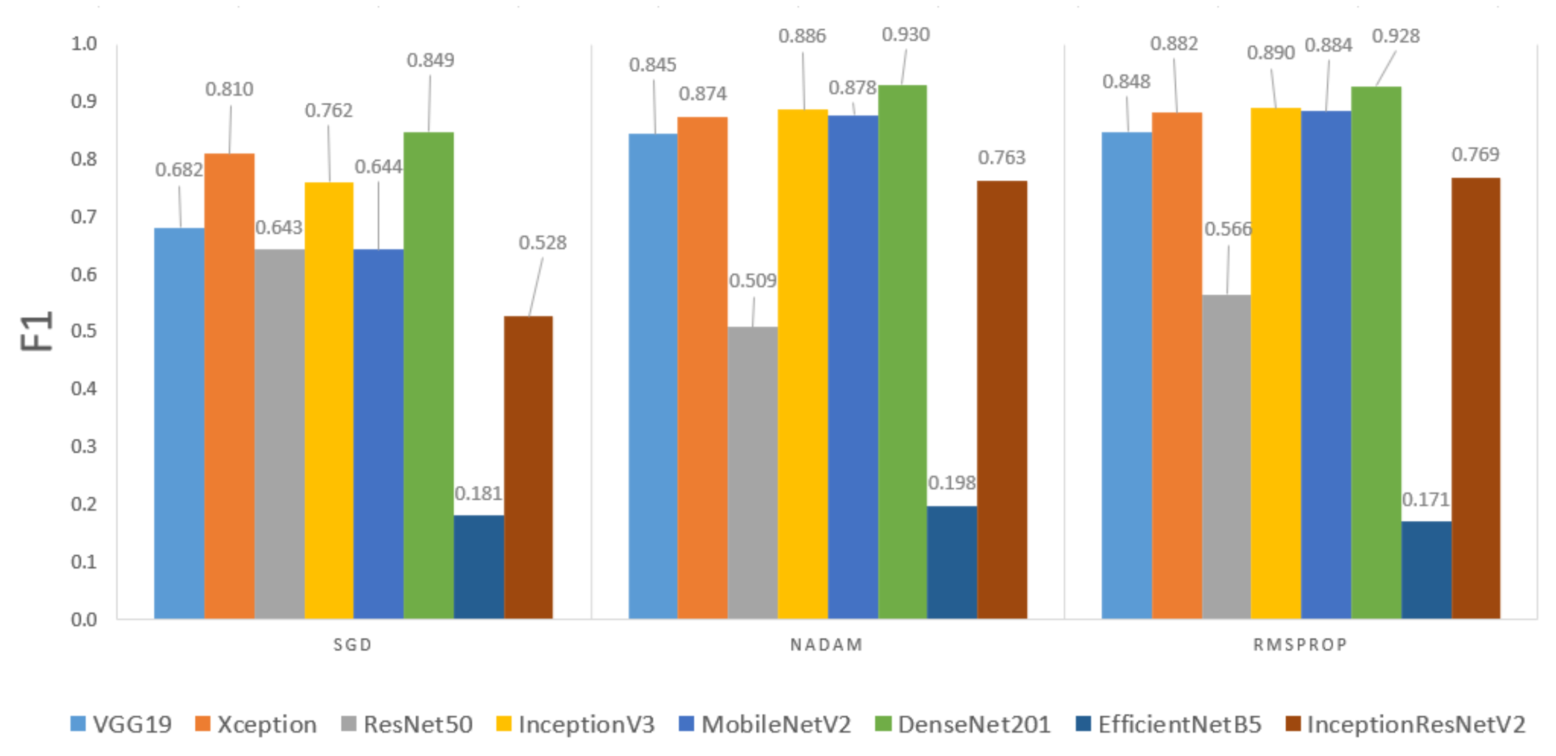
4.2. Evaluation by the Optimizer

Given the strong influence of the backbone used, the next step in the evaluation is to group the results by optimizer for each pre-trained network; it means grouped by 36 models in this study (see Figure 5). This is because an optimizer may work very well for one network but poorly for another, and the analysis must be performed separately.

For all the backbones selected in this study, except for ResNet50, the optimizer that provides the lowest F1-score is SGD. For example, when using MobileNetv2 as the backbone and SGD as the optimizer, the F1-score result is 64.4%, while when the optimizer is changed to RMSprop, the value is 88.4%. In another example, when using InceptionResNetV2 and SGD as the optimizer, the F1-score is 52.8%, but when the optimizer is Nadam, the value is 76.3%. The results obtained with Nadam and RMSprop are very similar to each other, and in general SGD is not a suitable optimizer for this type of classification problem.

In summary, this hyperparameter has a moderate impact on model performance (with variations of up to 25% among them).

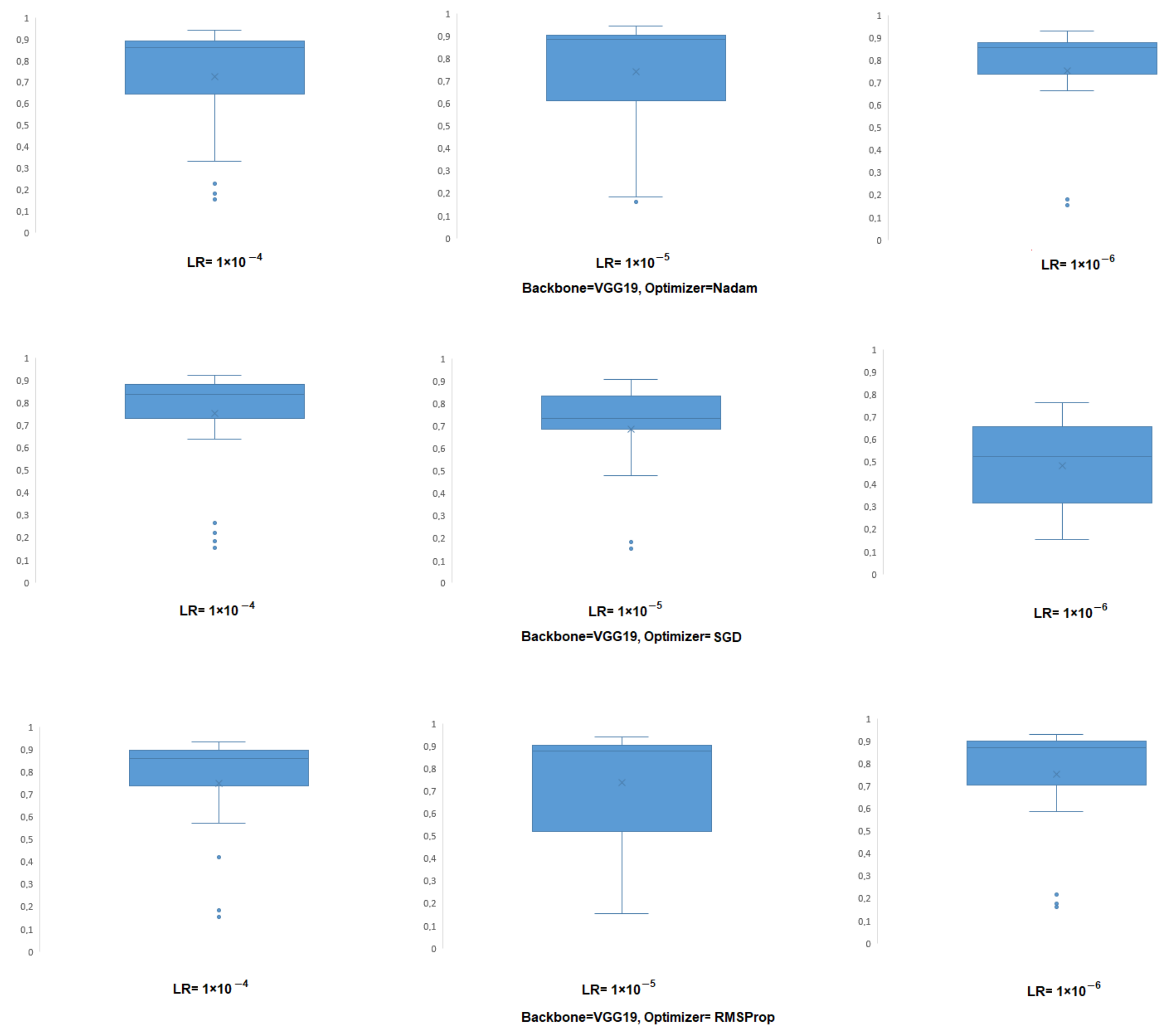
4.3. Evaluation by the Learning Rate (LR)

In association with the optimizer, the learning rate affects the performance of the classifier. Then it is necessary to know which LR value for each of the optimizers gives the highest F1-score results. Furthermore, this analysis must be performed for each backbone, grouping the models by the triplet [backbone, optimizer, and learning rate], i.e., by 12 models for this study.

As an example, Figure 6 shows the consolidated results for the VGG19 backbone, with the three optimizers, and for each of the learning rates. In each case, the box plot shows the average of the 48 cases, with their first and third quartiles, as well as the outliers. For the Nadam optimizer, when LR = $1\times {10}^{-6}$ (the lowest of the LRs selected in this study), the F1-score obtained with the 48 models has less dispersion among them compared with the results for LR = $1\times {10}^{-4}$ and LR = $1\times {10}^{-5}$. However, the highest F1-score for this backbone and optimizer is obtained for LR = $1\times {10}^{-5}$ (intermediate value of the LRs in this study). For the SGD optimizer, the results are the opposite of Nadam. In this case, the worst performance is obtained for the lowest LR (i.e., LR = $1\times {10}^{-6}$), while the best results are obtained for the highest LR (i.e., LR = $1\times {10}^{-4}$). Finally, for RMSprop, the greatest dispersion is obtained in the models that use the intermediate LR value (i.e., LR = $1\times {10}^{-5}$), but at the same time, it is with this value that the best F1-score is obtained.

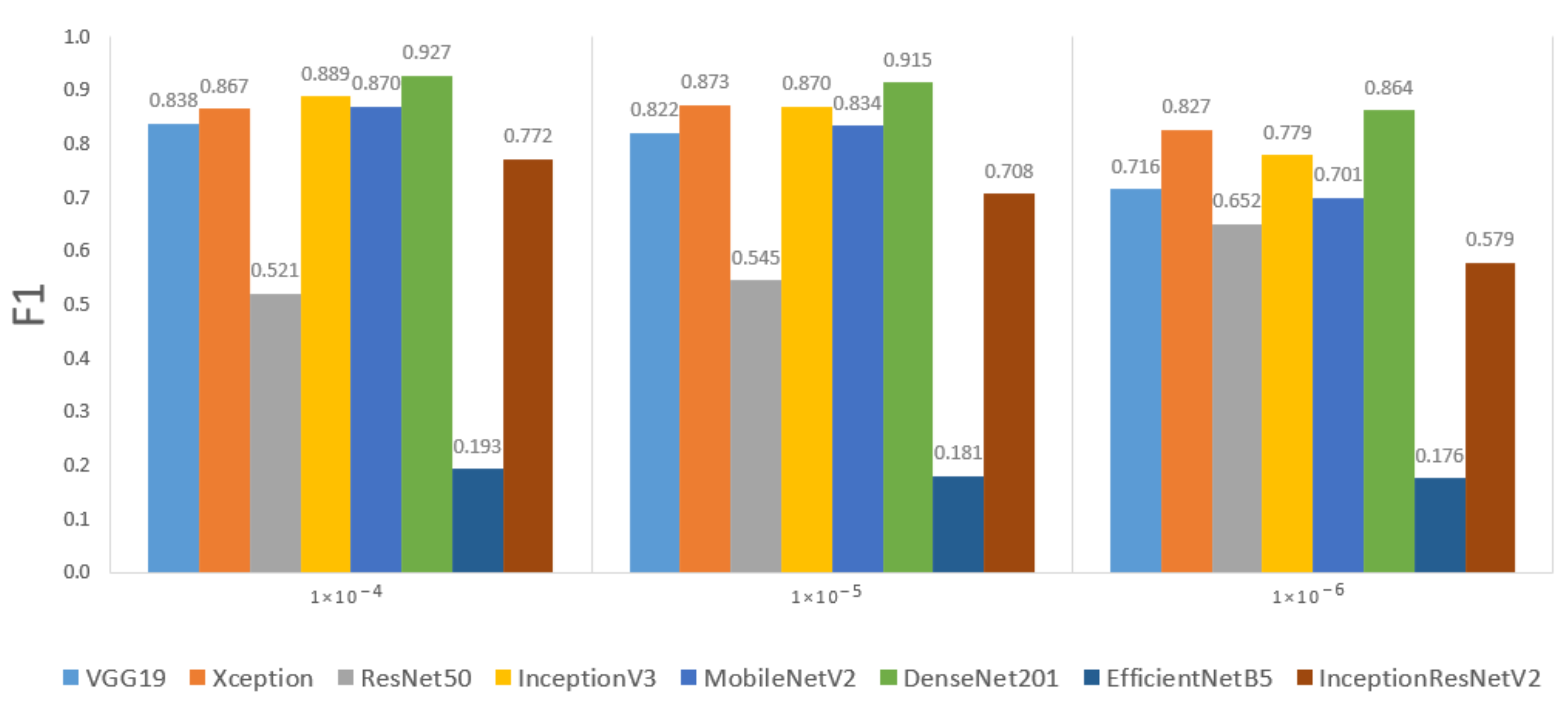
In the second part of the analysis of this hyperparameter, the results are grouped by LR value for each backbone, regardless of the optimizer used. The purpose is to see if one of the three LR values in the study generally gives better results than its competitors. The result is shown in Figure 7, where each bar represents 36 models.

According to the results obtained, for six of the eight backbones in this study, the average results are higher when using LR = $1\times {10}^{-4}$ (the higher of this study), with significant differences for some backbones. For example, for InceptionResNetV2, F1-score = 77.2% when LR = $1\times {10}^{-4}$ and drops to F1-score = 57.9% when LR = $1\times {10}^{-6}$. Another point to consider in Figure 7 is the slight increase of the F1-score value, in relation to the value of the learning rate for six architectures except ResNet50, which presents a decreasing trend, and for Xception architecture, where the highest value was obtained for the intermediate value (LR = $1\times {10}^{-5}$).

In summary, this hyperparameter has a moderate impact on model performance (with variations of up to 20% among them).

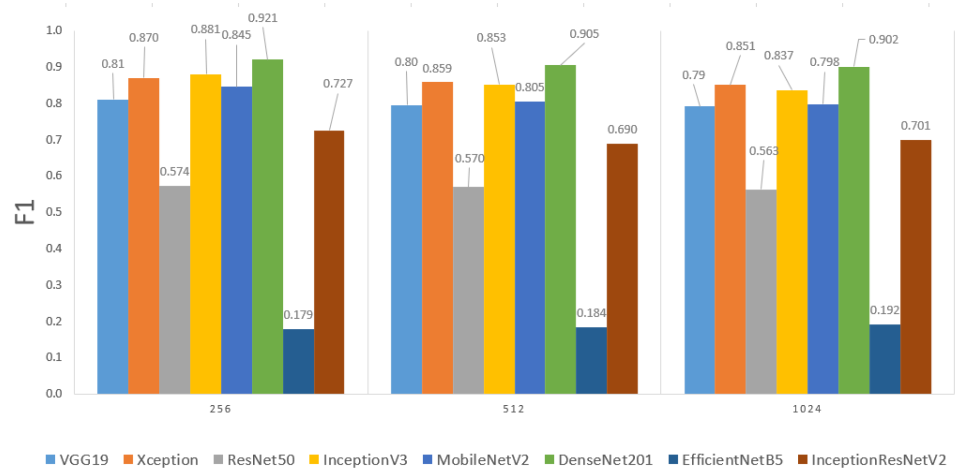
4.4. Evaluation by the Neurons in FC Layers

The next hyperparameter to analyze was the number of neurons in the top fully connected layers (except the output layer). Considering that the models are obtained by transfer learning with new FC layers (i.e., the FC layers of the pre-trained model are removed), this hyperparameter could affect the performance of the classifier for the dataset obtained in the collection and preparation phase.

Figure 8 shows the results grouped by the number of neurons in the FC layers (except for the output layer, which has three neurons). In this case, the differences between the three selected values of neurons for FC layers is very small. For example, when using VGG19 as backbone with 256 neurons the F1-score is 81.1%, for 512 neurons is 79.6% and for 1024 is 79.1%. These small differences also predominate in the other backbones. The difference between the best and worst result for the same backbone is up to 5% (i.e., using MobilNetV2 as backbone with 256 neurons the F1-score is 84.5% and with 1024 neurons is 79.8%. Considering that the results are slightly better when using 256 neurons in the FC layers, and also that the computational cost of training the models decreases, this is the value chosen for this architectural hyperparameter.

In summary, this hyperparameter has a low impact on model performance (with variations of up to 5% among them).

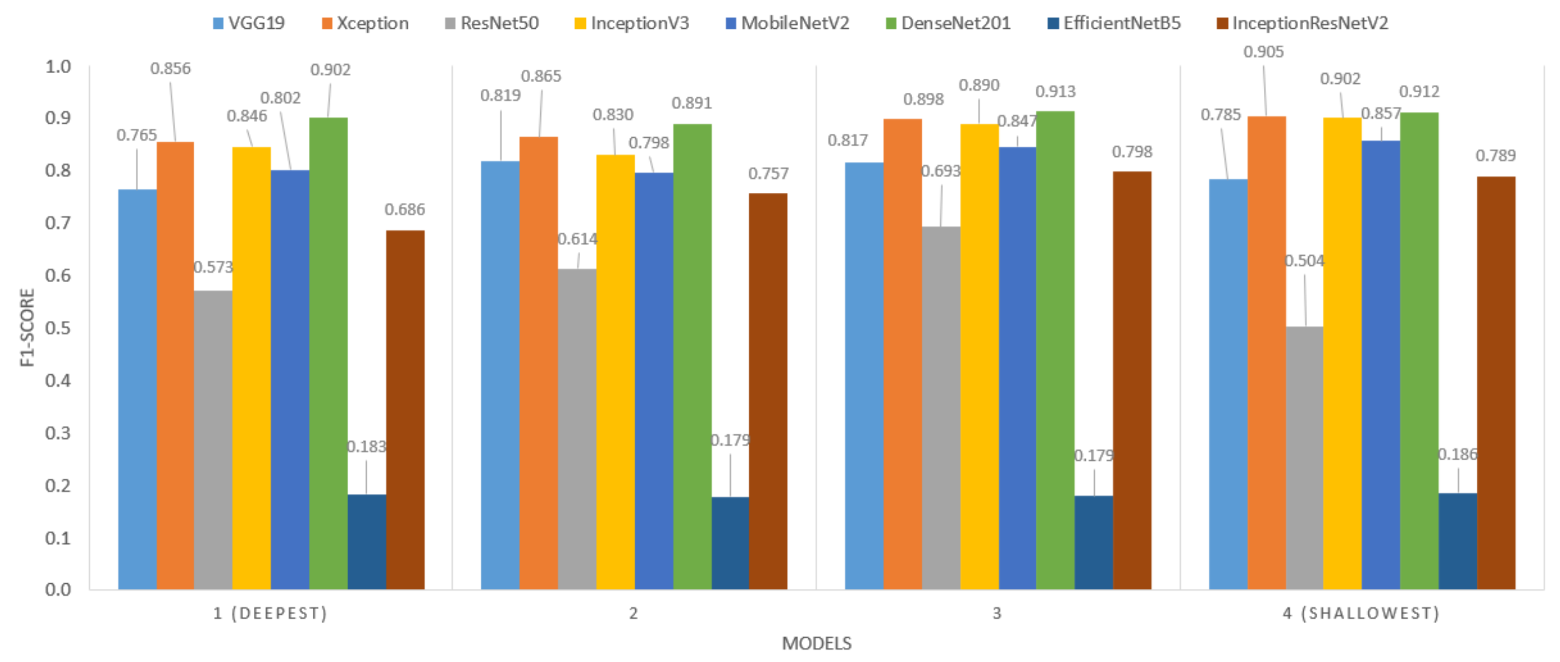
4.5. Evaluation by the Network Depth

When transfer learning is performed, the entire network (except the FC layers) or part of the convolutional layers can be transferred. Depending on the depth of the transferred network, the features extracted by the model will vary, such as edges, color, texture, shape, and others. Therefore, it is important to train the network at different depths, since not all classification problems make the decision with the same type of features.

For each of the backbones selected in this study, four depth levels were chosen, so that part of the convolutional network is transferred. For the analysis of this hyperparameter, the results were consolidated by backbone and network depth, with a total of 27 models for each case. Figure 9 shows the results.

Overall, the shallowest models perform best for Xception, InceptionV3, MobileNetV2, and DenseNet201. For VGG19, the best performance was produced with the second-deepest, while for ResNet50 it was the third. For EfficientNetB5, it has no significant impact. Although the impact of this hyperparameter is not as significant as some previous ones, it reaches differences between 2% and 3% for VGG19, Xception, or DenseNet201, and between 6% and 7% in InceptionV3 and MobileNetV2 architectures, for two different depth values. As a result, this hyperparameter showed a low impact on model performance (with variations of up to 7% between different depth levels).

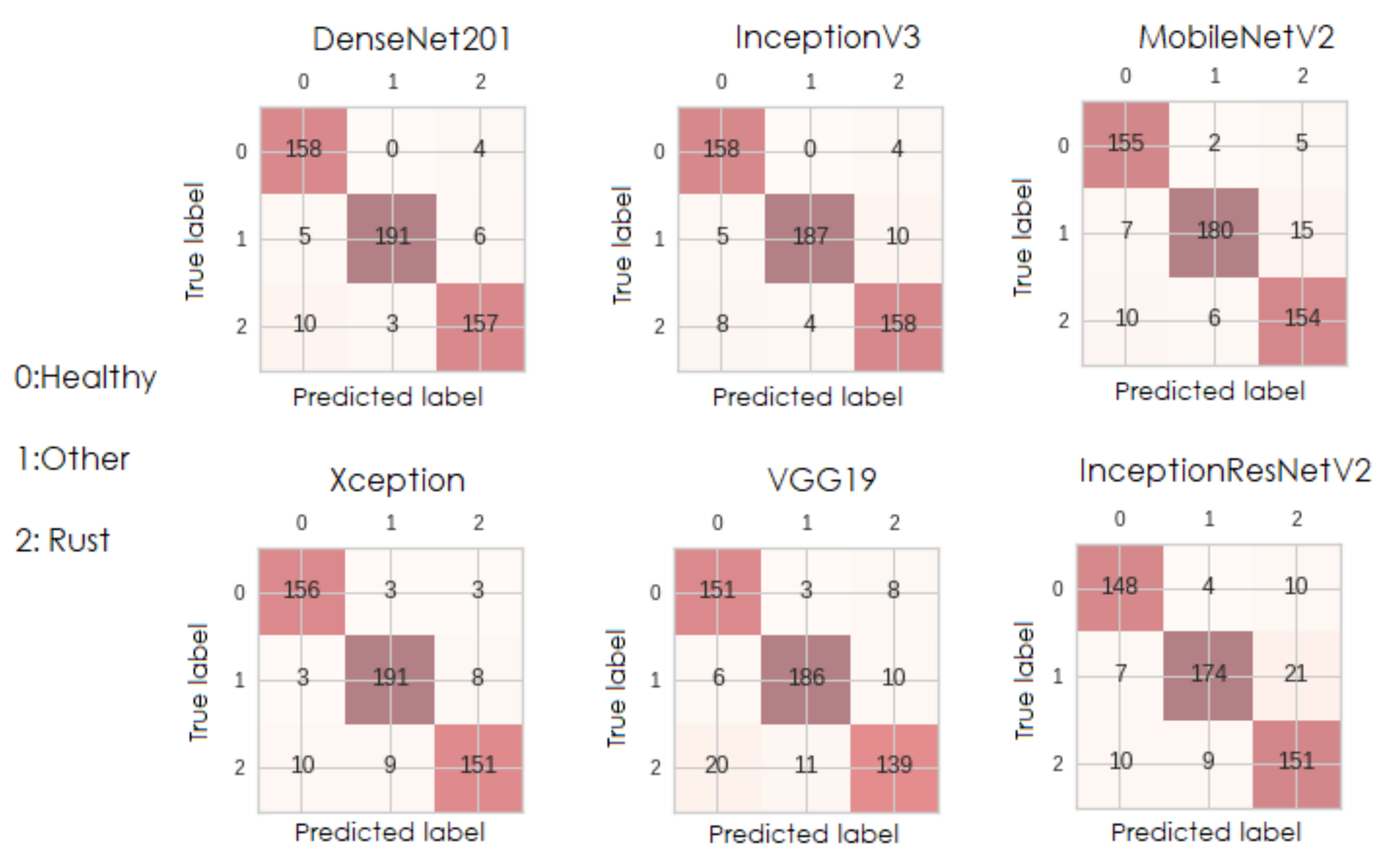
4.6. Comparison between the Best Models by Pre-Trained Network

Taking into account the validation results obtained in the previous section, the best model is chosen for each of the following backbones: DenseNet201, Xception, InceptionV3, MobileNetV2, VGG19, and InceptionResNetV2. For each trained model, inference was performed with the corresponding test images, and from the confusion matrices (Figure 10), four metrics were calculated, taking into account correct and incorrect classifications.

Table 5. Performance metrics on test data of the best classification model for each architecture. P is precision, R is recall, $F1$ is F1-score and $acc$ is accuracy. Values are in percentages, with 100% being the best result and 0% being the worst performance result.

Pre-Trained Model	Learning Rate	Neurons	Optimizer	P	R	F1	Acc
DenseNet201	$1\times {10}^{-5}$	256	Nadam	94.60	94.80	94.70	94.80
InceptionV3	$1\times {10}^{-5}$	256	RMSprop	94.10	94.30	94.20	94.20
Xception	$1\times {10}^{-4}$	256	RMSprop	93.20	93.20	93.20	93.30
MobileNetV2	$1\times {10}^{-4}$	256	RMSprop	91.50	91.80	91.60	91.60
VGG19	$1\times {10}^{-4}$	256	Nadam	88.90	89.00	88.90	89.10
InceptionResNetV2	$1\times {10}^{-4}$	256	RMSprop	88.57	88.77	88.59	88.58

presents the values of $acc$, P, R, and $F1$ for the best model from each backbone obtained by transfer learning.

Regarding the computational cost of the models,

Table 6. Classification models specification in terms of training time and size for models with the best result in present study.

Architecture	Last Layer	Time (s/epoch)	Avg ms/Step	Size (MB)	Param Num
Densenet201	conv5_block31_concat	112	93.2	219.1	30,112,963
Inceptionv3	mixed6	329	135.5	263.9	26,494,243
Xception	block13_sepconv1_act	398	310.0	378.7	40,899,419
MobileNetv2	block_14_add	30	25.9	16.9	2,066,755
VGG19	block4_pool	82	90.0	269	29,461,571
InceptionResnetv2	block8_8_mixed	177	59.3	199	47,164,995

presents the name of the last layer transferred, the training time of each epoch/step, the size in MB, and the number of model parameters. From this point of view, it is clear that VGG19 and MobileNetv2 are the fastest models to train, and the latter is significantly one of the lightest models in terms of disk size and number of parameters. Although the F1-score performance of these two models is relatively competitive, it is slightly lower than those obtained from DenseNet201 and InceptionV3.

5. Discussion

In several state-of-the-art manuscripts that use transfer learning for disease identification, specifically coffee leaf rust, ResNet has been used as a backbone [13,15,43]. Specifically in [15], the authors use ResNet with two approaches: raw images from the RoCoLe dataset and a mixture between segmented and patches of the original images. Their results are 75% and 98% of accuracy, respectively. It is important to mention this paper since in our study it was found that the models obtained using ResNet50 as a backbone have an accuracy of less than 70%, whose results are significantly lower than models obtained with another type of backbone, such as DenseNet201, whose values of accuracy are greater than 90% (see Table 6). This evidences the importance of carrying out a comprehensive study of the impact of the backbone used in crop disease recognition problems, given that, according to our results, it is the hyperparameter with the greatest impact on the performance of the classifier. Additionally, it is emphasized that the values obtained with ResNet in [15] are slightly higher than those obtained in this study for the same type of backbone, since they used a single dataset (i.e., RoCoLe), while our research used images from five different datasets (i.e., Bracol, RoCoLe, D&P, Digipathos, and Licole) with diversity of light conditions, image size, type of background, among others.

On the other hand, some state-of-the-art works have made a comparison of different backbones, but with a low number of pre-trained networks or by leaving out those that have high Top1-accuracy values for the ImageNet dataset. For example, the article by [13] compares five backbones (AlexNet, GoogleNet, VGG16, ResNet50, and MobileNetV2), where none of them have a Top1-accuracy above 75%, leaving out pre-trained models such as InceptionResNetV2 (80.3%), Xception (79%), ResNet152V2 (78%), DenseNet201 (77.3%), NASNetLarge (82.5%), EfficientNetB7 (84.3%), among others. It is important to note that according to the results (see Figure 4), the pre-trained networks that present high values of Top1-accuracy (with the ImageNet dataset) are the ones that obtained the highest values of accuracy, precision, recall, and F1-score for our dataset obtained from Bracol, RoCoLe, D&P, Digipathos, and Licole.

It should be noted that in similar works, the optimizer is a hyperparameter that is left fixed, e.g., SGD [13] or RMSprop [15]. However, this type of hyperparameter has the second-highest impact on model performance, with variations of up to 20% in accuracy. According to the results (see Figure 4), the models that used SGD obtained significantly lower results than those obtained with Nadam and RMSprop. Therefore, it is necessary not only to select a suitable model as the backbone, but also the optimizer with which the fine-tuning of the network will be carried out for the new dataset. The third hyperparameter in order of importance was the learning rate (suggesting that its value is greater than $1\times {10}^{-5}$). For the set of hyperparameters evaluated, it was found that the number of neurons in the FC layer and the depth of the model ranked fourth and fifth in model impact. Overall, 256 neurons in the FC layer and shallower models performed better.

It is observed that the best models obtained in this study, whose results are presented in Table 5, have the four metrics (P, R, F1, and Acc) very similar to each other, with differences of less than 0.3%, for example, for DenseNet201, it is obtained that P = 94.60%, R = 94.80%, F1-score = 94.70% and Acc = 94.80%. This implies that the models are unbiased, i.e., they classify equally well in all classes. Furthermore, the model with the best performance (DenseNet201) according to Table 5 corresponds to the model with the lowest dispersion among the architectures evaluated in Figure 6.

Due to the conformation of a dataset from diverse datasets available in the literature, we inferred that the best models were less influenced by the covariance change factor [7,11] compared with previous works using a specific dataset in their work [14,16,19,20,21], therefore, the importance of the proposed methodology for the selection of a coffee leaf rust classification model applicable to other types of crops is emphasized.

Finally, the lower performance presented in the EfficientNetB5 and ResNet50 models observed in the present study, along with the slight trend of increasing performance values relative to decreasing LR for ResNet50, could be due to the fact that the search space may have left out the best values for these models, in agreement with what was presented by Martinez et al. [16]. Therefore, it may be necessary to expand this space for these specific models and analyze the change in covariance for the coffee leaf rust classification.

6. Conclusions

When realizing image classification solutions using models that learn from data, there are two main approaches: data-centric and model-centric. In the state-of-the-art of coffee leaf rust recognition, many solutions have been focused on data pre-processing, for example, by including patches from the raw images, deleting the background, and cropping the image, among others. However, little has been discussed about the impact of hyperparameters, and solutions have used values that are not necessarily the most appropriate for this specific problem (for example SGD as optimizer). For this reason, it is necessary to have exhaustive studies of the impact of hyperparameters that allow selecting the best ones for coffee leaf rust recognition using transfer learning. According to the results of the more than 800 trained models, the type of backbone used is the most important hyperparameter, since the variations between the models can reach 70% in terms of accuracy. In second place is the optimizer, with variations of up to 20% between the three optimizers used. Finally, the learning rate is the third most important hyperparameter, with variations of 10% in some cases, although its impact depends largely on the optimizer and the pre-trained network used as the backbone. Other types of hyperparameters, such as the number of neurons in the FC layer before classification and the depth of the model, had less impact with respect to the other three parameters evaluated. It is recommended to use 256 neurons due to the computational cost and shallower models with respect to the base models obtained by transfer learning.

The presented methodology concludes with different suitable models based on different architectures, including practical considerations to be applied to coffee leaf rust classification problems on a diverse dataset. In consideration, and although model architectures are not defined as hyperparameters in the literature, they could be handled as one of them.

7. Future Work

In future work, it is proposed to integrate the data-centric approach with the model-centric approach to improve the classification results of coffee leaf images in the three categories defined in this study: healthy, other, and rust. That is, select the four best models (taking into account the type of backbone, optimizer, learning rate, number of neurons, and depth of the network) related to this study, and apply new pre-processing tasks to the dataset, for example, creating patches of the images with automatic sizes according to the type of information contained, for example, small when there is rust and larger when the leaf is healthy. The above helps generate a solution that includes an attention mechanism and thus improves decision-making by the model.