Steel Arch Support Deformations Forecast Model Based on Grey–Stochastic Simulation and Autoregressive Process

Abstract

Relatively large deformations of the steel arch support in underground coal mines in the Republic of Serbia present one of the main problems for achieving the planned production of coal. Monitoring of the critical sections of the steel arch support in the underground roadways is necessary to gather quality data for the development of a forecasting model. With a new generation of 3D laser scanners that can be used in potentially explosive environments (ATEX), deformation monitoring is facilitated, while the process of collecting precise data is much shorter. In this paper, we used a combination of grey and stochastic system theory combined with an autoregressive process for processing collected data and the development of a forecasting model of the deformations of the steel arch support. Forecasted data accuracy based on the positions of the markers placed along the internal rim of support construction shows high accuracy with MAPE of 0.2143%. The proposed model can successfully be used by mining engineers in underground coal mines for steel arch support deformations prediction, consequentially optimizing the maintenance plan of the underground roadways and achieving planned production.

1. Introduction

For the process of production of mineral resources in underground mines to proceed smoothly, it is necessary to ensure the functionality and stability of the underground rooms. Sometimes, to ensure both functionality and stability of the underground roadways, which are directly related, it is necessary to install a suitable support substructure. The support takes static and dynamic loads from the rock mass and begins to deform over time. For the unhindered passage of loading and transport machinery, it is necessary to design the underground roadway considering the minimum dimensions of the free cross-section of the underground roadway, including the legally defined minimum safety distances from the equipment to the walls and roof of the roadway. As time passes, the underground support suffers deformations, and it can happen that the minimum dimensions are violated, after which the transportation and export of useful mineral resources are suspended. In such cases, it is necessary to proceed with the reconstruction of the underground roadway, which can have a significant impact on the economic operation of the mine, because the reconstruction is both a financially and time-consuming process that impairs continuous production. To avoid such situations, it is necessary to conduct systematic monitoring of deformations of the support construction and provide a forecast of deformations. With proper forecasting, mining engineers can react in a timely manner and plan the replacement of the underground support in the necessary sections of the underground roadway. In this way, strategic management of the functionality of underground rooms and continuous production is achieved. The use of a laser scanner or similar instrument with the possibility of gathering high-accuracy data is necessary to obtain deformation data that can be used for analysis and forecasting the future states of the support construction.

Various approaches can be used to obtain future states of support construction. Deformation forecast has been the subject of research by many authors, with different approaches for prediction of tunnel surrounding rock displacement, structural deformations prediction, deformations of the lake bottom, landslide deformations, slope deformations, displacements of mining roadways, and so on. Wu et al. [1] used two methodologies, support vector machines and artificial neural networks, to predict tunnels surrounding rock displacements; though the support vector machine gave more accurate predictions, it was more time-consuming than the artificial neural network. Luo et al. [2] proposed a model based on temporal convolutional networks in their study for structural deformation prediction, which they verified with the cumulative strain data of the upper steel beam in the foundation pit in China as well as the structural subsidence data on the same location. Luan et al. [3] showed that the grey model GM(1,1) could be used for the prediction of the deformations on the lake bottom. Ma et al. [4] used tunnel geological information as well as monitoring measurement data to determine factor weights, and extension theory was used for the prediction model of tunnel deformations. In their study, Rao et al. [5] used the grey model theory for the prediction of the large deformation of the tunnel. Guo et al. [6] established a grey forecast model for rock deformation in a big tunnel cross section and concluded that it could be used in engineering practice. Prediction of the final displacement of underground structures based on the improved no equidistant grey Verhulst model was used by Han et al. [7]. Xiong [8] predicted displacements in tunnels surrounding rock using the grey system theory. For landslide deformations, displacements were predicted by a model combining extreme learning machines and grey wolf optimization by Zhang et al. [9], and by using a new grey model prediction by Wu et al. [10] as well as Li and Wu [11]. Slope deformation prediction was calculated using the grey model by Li et al. [12] and Zhang et al. [13]. In the mining environment, multivariate singular spectrum analysis was used by Crnogorac et al. [14] for accurate gate road support deformation forecasting. Zhu et al. [15] proposed mining roadway displacement forecasting using the support vector machine theory. Xie et al. [16] used a grey algebraic curve model for the prediction of the roof fall.

The aim of this paper is to develop an accurate grey forecasting algorithm for coal mines where large deformations of support constructions occur in a relatively short period of time. These deformations are the result of high underground pressure which occurs around the underground roadways, and the main factors for the occurrence of high underground pressure are bad geological conditions and poor physic-mechanical properties of the surrounding rock mass, as well as the presence of the clay which swells when in contact with water, adding additional pressure to support construction. In underground coal mines in the Republic of Serbia, the most used support for underground roadways is steel arch supports, followed by steel circular and wooden supports. Because of this, in our paper, we will focus on the deformations forecast in the case of the application of steel arch supports in underground roadways.

This paper has four sections. In the section Materials and Methods, the forecasting model of displacements of the steel arch support based on the grey system (1,1) and stochastic theory is described. A novel approach is used that considers the displacements of the markers along the steel arch support that better describes the real situation (an example was given for marker M4 and its movement along the x coordinate in both directions). Using grey–stochastic simulation and the autoregressive process, the configuration of the steel arch support was described and forecasted based on the observed data. For error estimation of the model due to the nature of the problem we described, besides the usual MAPE error approach, which deals with displacements of the marker along the x and y axes as two separated time series and does not consider the fitted position of the marker, we introduced the novel approach of model accuracy dealing with the analysis of the closeness between fitted and observed position of the marker. The calculation process is shown in the section Numerical Example to represent the possibilities of this model. All steps of the calculation in the section Numerical Example are discussed, and the results, efficiency, and the area of implementation of the model are represented. Results show that the model is capable, and it can be used, to solve real-time problems concerning the forecasting deformations of the steel arch support in underground coal mines.

2. Materials and Methods

2.1. Displacement of the Steel Arch Support

Due to the influence of the rock stress surrounding the underground roadway that is supported by steel arch support, deformations occur on the support construction. Time-dependent response of support construction under dynamic loads from the rock mass represents the dynamic of the displacement. Changes in underground pressure are the result of mining operations and are manifested by changing loads that the steel arch support bears.

To describe the deformations, we will monitor the displacement of the seven markers that are positioned along the lower edge of the steel arch support. Like in our previous research, without a loss of generality, we can make the upper and lower edge of the steel arch support equal, transforming the two-dimensional steel arch support into one-dimensional support [14].

Starting configuration of the steel arch support will be described with the starting coordinates (x, y) that are recorded by 3D laser scanner. Displacements in time represent vectors that can be described in any moment with positions on the x- and y-axis. It is especially important that all recorded data are in the same coordinate system.

Displacement of the markers along x- and y-axis will be monitored in equal intervals to define positions of the markers in time and, by that, the deformations of the support construction.

Figure 1 represents the positions of the markers (t = 0) and their displacements (t = 1).

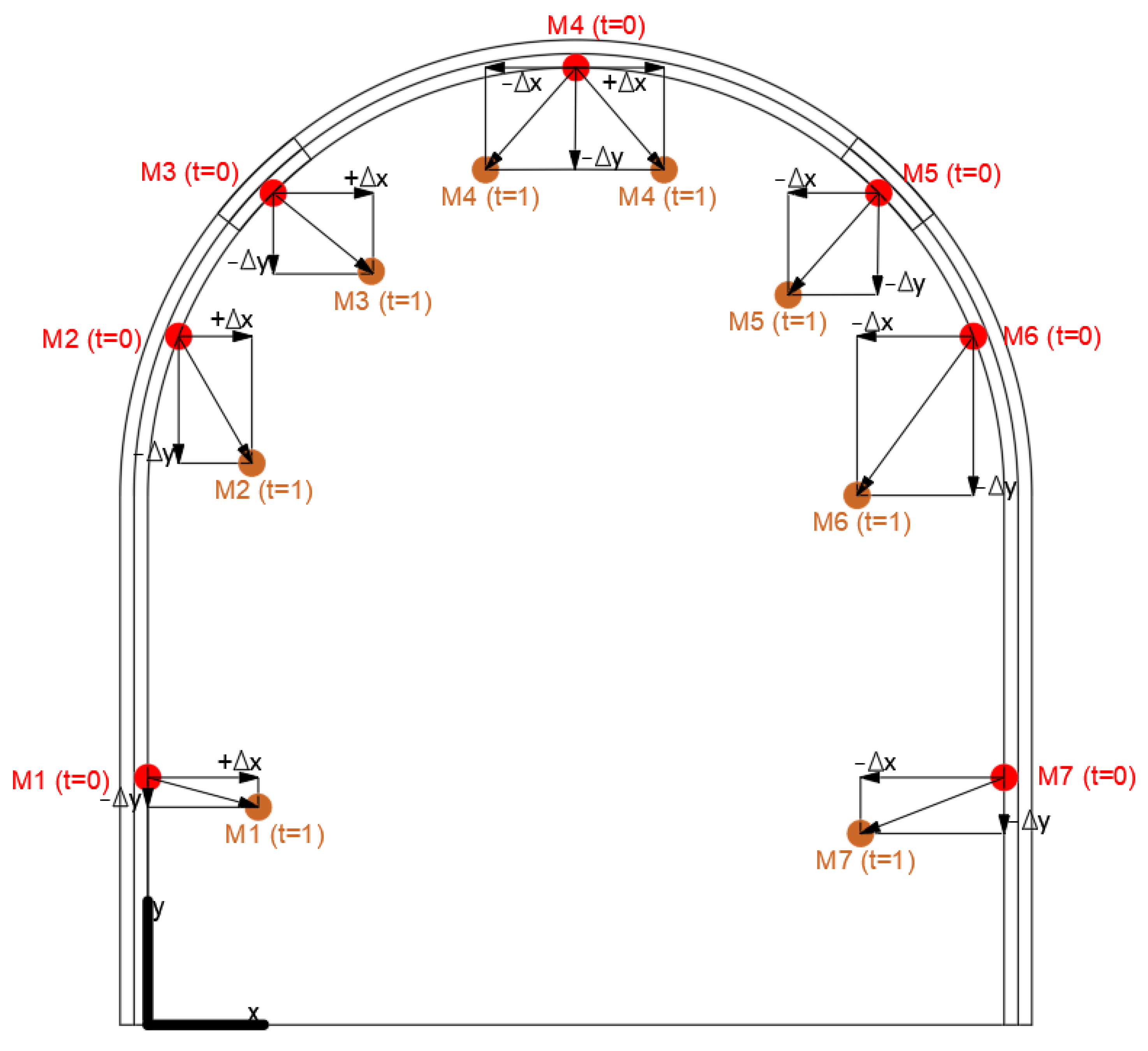
Figure 1. Positions of the markers (t = 0) and their displacements (t = 1).

As seen from Figure 1, markers 1, 2, and 3 can change their positions with coordinates along y-axis with negative sign (−Δy) and along the x-axis with positive sign (+Δx). Marker 4 will change its coordinates in time by y-axis in negative sign (−Δy), and changes along the x-axis are expected to occur in both negative and positive directions (−Δx and +Δx). Markers 5, 6, and 7 will have negative signs for changes both along the y-axis (−Δy) and x-axis (−Δx).

Positions of the markers in time are described by the equation

$$\begin{array}{c}{M}_i\left(t=0\right)=\left\{x_{io};y_{io}\right\},\forall i\in \left[1,N\right]\\ M_i\left(t=1\right)=\left\{x_{io}\pm ∆x\left(t=1\right);y_{io}-∆y\left(t=1\right)\right\},\forall i\in \left[1,N\right]\\ ⋮\\ M_i\left(t\right)=\left\{x_i(t-1)\pm ∆x\left(t\right);y_i(t-1)-∆y\left(t\right)\right\},\forall i\in \left[1,N\right]\end{array}$$

(1)

where N represents the total number of markers.

The changes in the shape of steel arch support for a defined time interval (0, t) can be displayed via the marker union as follows:

$$\bigcup _{i=1}^N{M}_i\left(t\right),\forall t\in \left[0,T\right]$$

(2)

where T represents the monitoring time interval, and for t = 0, x_i and y_i are the initial coordinates for the i-th marker.

2.2. The Model of Support Deformation Forecasting

2.2.1. Fitting the Monitored Displacements

The proposed model of support deformation forecasting will be explained with respect to displacement of one marker M along x-axes. Let us consider a monitored time series of marker displacement along x-axes over time $t=\mathrm{1,2},\dots ,T$. Denote monitored time series as $∆X\left(t\right)=\left({∆x}_1,{∆x}_2,\dots ,{∆x}_T\right)$. Next, we define three different states of displacement series, namely non-negative, negative, and mixed. The series is in the non-negative state if all values of ${∆x}_t$ are greater than zero, while the series is in the negative state if all values of ${∆x}_t$ are smaller than zero. Values greater and smaller than zero are considered mixed series. The value of zero is rare and will not be included in modeling. Hence, define

$${∆x}_t=\left\{\begin{array}{l}NN,if{∆x}_t>0\\ N,if{∆x}_t<0\\ MD,if{∆x}_t>0\wedge {∆x}_t<0\end{array}\right.$$

(3)

The model can deal with NN and N state of series, while MD state must be transformed into NN state. First, we define the vector of transformation coefficients for MD state as follows:

$$K\left(t\right)={\left\{k_t\right\}}_{T\times 1}=\left\{\begin{array}{l}1,if{∆x}_t>0\\ -1,if{∆x}_t<0\end{array},t=\mathrm{1,2},\dots ,T\right.$$

(4)

Furthermore, we make product of k_t and ${∆x}_t$, and result is transformed mixed state of series (TMD), shown below:

$$TMD\to NN=\left[\begin{array}{c}{k}_1{∆x}_1\\ k_2{∆x}_2\\ k_3{∆x}_3\\ ⋮\\ k_t{∆x}_t\end{array}\right],t=\mathrm{1,2},\dots ,T$$

(5)

From this point, we continue to model the original NN and N state of series, and TMD state of series, in the same way. To obtain stationary displacement series, it is necessary to calculate the first order differencing of non-negative or negative state of series $∆X\left(t\right)$. For the first difference, we write the following:

$$∆\left(∆x_t\right)={∆x}_t-{∆x}_{t-1},t=\mathrm{2,3},\dots ,T$$

(6)

The result is stationary time series, and we can model the first difference, $∆\left(∆x_t\right),t=\mathrm{2,3},\dots ,T$, instead of level of ${∆x}_t$. Denote differenced series $∆\left(∆x_t\right)$ as $Q\left(t\right)=\left[q_t\right],t=\mathrm{2,3},\dots ,T$, where $q_t={∆x}_t-{∆x}_{t-1},t=\mathrm{2,3},\dots ,T$. To avoid confusion about denoting the time, we map differenced series into new regular one Q(t), and it is shown below.

$$∆X\left(t\right)=\left[\begin{array}{cc}t=1& {∆x}_1\\ t=2& {∆x}_2\\ t=3& {∆x}_3\\ ⋮& ⋮\\ t=T& {∆x}_T\end{array}\right]\stackrel{diff.}{\to }\left[\begin{array}{cc}t=2& {q_2=∆x}_2-{∆x}_1\\ t=3& q_3={∆x}_3-{∆x}_2\\ ⋮& ⋮\\ t=T& q_t={∆x}_T-{∆x}_{T-1}\end{array}\right]\stackrel{Map}{\to }Q\left(t\right)=\left[\begin{array}{c}{q}_1\\ q_2\\ ⋮\\ q_T\end{array}\right]$$

(7)

The number of elements in the new mapped series is less than in monitored series, for one. The first order difference produces a time series consisting of negative and non-negative values, i.e., MD state of differenced series. It shows the necessity for transformation from state MD to state NN. Applying Equations (2) and (3) on series Q(t), we obtain Q(t) as NN state. For simplicity, denote NN state of Q(t) series as P(t). In this way, we processed data to be modeled by the Grey system theory.

The Grey system model GM(1,1), where first “1” denotes the order of derivative, and the second “1” denotes one-dimensional variable, will be used to fit and forecast the series $P\left(t\right)$ [17,18,19,20].

For a series $P\left(t\right)=\left(p_1,p_2,\dots ,p_T\right)$, a monotonically increasing cumulative series is defined as follows:

$$P^{\left(1\right)}\left(t\right)=\left\{p_1^{\left(1\right)},p_2^{\left(1\right)},\dots ,p_T^{\left(1\right)}\right\}$$

(8)

Elements of a cumulative series are calculated by Accumulated Generation Operation (AGO) as follows:

$$p_t^{\left(1\right)}=\sum _{i=1}^t{p}_i,t=\mathrm{1,2},\dots ,T$$

(9)

where $p_1^{\left(1\right)}=p_1$, $p_2^{\left(1\right)}=p_1+p_2$, $p_3^{\left(1\right)}=p_1+p_2+p_3$, and so forth.

Mean value of neighboring values of a series $P^{\left(1\right)}\left(t\right)$ is calculated in the following way:

$$z_t^{\left(1\right)}=\frac{1}{2}\left(p_t^{\left(1\right)}-p_{t-1}^{\left(1\right)}\right),t=\mathrm{2,3},\dots ,T$$

(10)

The grey system model is described by the differential equation:

$$\frac{d{p}_t^{\left(1\right)}}{dt}+a{p}_t^{\left(1\right)}=b$$

(11)

The parameters a and b are estimated according to the least square criterion,

$${\left[\begin{array}{cc}a& b\end{array}\right]}^T=\underset{a,b}{\underbrace{\mathit{arg}min}}{‖\mathit{Y}-\mathit{B}{\left[\begin{array}{cc}a& b\end{array}\right]}^T‖}_2^2={\left({\mathit{B}}^T\mathit{B}\right)}^{-1}{\mathit{B}}^T\mathit{Y}$$

(12)

where

$$\mathbf{B}=\left[\begin{array}{cc}{-z}_1^{\left(1\right)}& 1\\ -z_2^{\left(1\right)}& 1\\ ⋮& ⋮\\ {-z}_T^{\left(1\right)}& 1\end{array}\right],\mathbf{Y}=\left[\begin{array}{c}{p}_2\\ p_3\\ ⋮\\ p_T\end{array}\right]$$

(13)

Equation (11) presents ordinary differential equation of the form:

$${dp}_t^{\left(1\right)}=f\left(t,p_t^{\left(1\right)}\right)dt$$

(14)

with initial condition $p_{t=1}^{\left(1\right)}=p_1$. Displacement is subject to random perturbation caused by random variation of the loading forces over time. It is hard to specify it in the model description, working within the system. Such perturbations create noise in the monitored displacements and AGO series as well, and cannot be captured by Equation (14). When we take Equation (14) and assume that $f\left(t,p_t^{\left(1\right)}\right)$ is not deterministic function but stochastic, and add the noisy part to it, we obtain stochastic differential equation. So, we can create stochastic differential equation with additive noise part as follows:

$${dp}_t^{\left(1\right)}=f\left(t,p_t^{\left(1\right)}\right)dt+d{W}_t,t=\mathrm{1,2},\dots ,T$$

(15)

where:

$d{W}_t$—Brownian motion, $d{W}_t~N\left(0,Var\right)$

The grey system model is now transformed into stochastic system [21]

$${dp}_t^{\left(1\right)}=\left(b-a{p}_t^{\left(1\right)}\right)dt+{dW}_t,p_{t=1}^{\left(1\right)}=p_1$$

(16)

Numerical approximation of $p_t^{\left(1\right)}$ is obtained from the explicit Euler–Maruyama discretization [22]:

$$p_t^{\left(1\right)}=p_{t-1}^{\left(1\right)}+\left(b-a{p}_{t-1}^{\left(1\right)}\right)∆t+∆W_t,t=\mathrm{1,2},\dots ,T$$

(17)

using a uniform timestep of $∆t$ with Brownian increments $∆W_t$, and there is a fixed initial value $p_{t=1}^{\left(1\right)}=p_1$. Behavior of $p_t^{\left(1\right)}$, in the form of Equation (17), is only discrete in the time variable but not as random variable. Set $∆t=\frac{T}{\phi },\phi \le T$ and $∆W_t=W_t-W_{t-1}~N\left(0,\frac{{\sigma }^2}{\omega }\right)$, where $\phi$ is the number of timesteps in time T and $N\left(0,\frac{{\sigma }^2}{\omega }\right)$ is the normal distribution with expected value of 0 and variance $\frac{{\sigma }^2}{\omega }$. Variance in AGO series is ${\sigma }^2$ and $\omega$ is the time resolution coefficient, which is defined as follows:

$$\omega =\left\{\begin{array}{l}1,annualtimeresolution\\ 12,monthlytimeresolution\\ 365,dailytimeresolution\end{array}\right.$$

(18)

Substituting $∆W_t~N\left(0,\frac{{\sigma }^2}{\omega }\right)$ in Equation (17), we obtain solution of the stochastic AGO process defined by Equation (16):

$$p_t^{\left(1\right)}=p_{t-1}^{\left(1\right)}+\left(b-a{p}_{t-1}^{\left(1\right)}\right)∆t+N\left(0,\frac{{\sigma }^2}{\omega }\right),t=\mathrm{1,2},\dots ,T$$

(19)

Assume we have a function, f: ℝ→ℝ, which depends on the solution, $p_t^{\left(1\right)}$, of the stochastic differential Equation (16) on the time interval [1,T]. Equation (19) presents the solution, and simulation of Equation (19) produces expected values for specific point in time of the AGO stochastic process:

$${\mathrm{E}}_t^{AGO}=\frac{1}{S}{\displaystyle \sum _{s=1}^S}{p}_{t,s}^{\left(1\right)},t=\mathrm{2,3},\dots ,T,{\mathrm{E}}_1^{AGO}=p_1$$

(20)

where

S—the total number of simulations.

Obviously, at every point in time, there is an adequate probability density function of AGO. Next, the Inverse Accumulated Generation Operation (IAGO) is applied to reconstruct NN state of P(t) series as

$$\left\{\begin{array}{l}{\mathrm{E}}_{t+1}^{IAGO}={\mathrm{E}}_{t+1}^{AGO}-{\mathrm{E}}_t^{AGO},t=\mathrm{1,2},\dots ,T-1\\ {\mathrm{E}}_1^{IAGO}=p_1\end{array}\right.$$

(21)

Reconstructed (fitted) NN state of P(t) series is of the following form:

$$\widehat{P}\left(t\right)=\left(p_1,{\widehat{p}}_2,\dots ,{\widehat{p}}_t\right),t=\mathrm{1,2},..,T$$

(22)

Let us remember that NN state of P(t) series equals the NN state of Q(t) series. Hence, fitted NN state of Q(t) series is

$$\widehat{Q}\left(t\right)=\left(q_1,{\widehat{q}}_2,\dots ,{\widehat{q}}_t\right),t=\mathrm{1,2},..,T$$

(23)

By nature, $\widehat{Q}\left(t\right)$ series is MD (mixed) series, and transformation from NN to MD state is performed by applying Equation (5) on $\widehat{Q}\left(t\right)$ series,

$$MD\widehat{Q}\left(t\right)=k_t^q{\widehat{q}}_t,t=\mathrm{1,2},\dots ,T,{\widehat{q}}_t>0$$

(24)

where

$$K^q\left(t\right)={\left\{k_t^q\right\}}_{T\times 1}=\left\{\begin{array}{l}1,if{q}_t>0\\ -1,if{q}_t<0\end{array},t=\mathrm{1,2},\dots ,T\right.$$

(25)

For original NN and N state of series, reconstructed (fitted) series of displacement is as follows:

$$∆\widehat{X}\left(t\right)={\left\{{∆\widehat{x}}_t\right\}}_{T\times 1}=\left[\begin{array}{c}{∆\widehat{x}}_2\\ {∆\widehat{x}}_3\\ {∆\widehat{x}}_4\\ ⋮\\ {∆\widehat{x}}_t\end{array}\right]=\left[\begin{array}{c}{∆x}_1+k_1^q{q}_1\\ {∆x}_2+k_2^q{\widehat{q}}_2\\ {∆x}_3+k_3^q{\widehat{q}}_3\\ ⋮\\ ∆x_{t-1}+k_t^q{\widehat{q}}_t\end{array}\right],t=\mathrm{2,3},\dots ,T$$

(26)

For original MD state of series, fitted series of displacement is calculated as:

$$∆\widehat{X}\left(t\right)={\left\{{∆\widehat{x}}_t\right\}}_{T\times 1}=\left[\begin{array}{c}{∆\widehat{x}}_2\\ {∆\widehat{x}}_3\\ {∆\widehat{x}}_4\\ ⋮\\ {∆\widehat{x}}_t\end{array}\right]=\left[\begin{array}{c}{k}_2\left|{∆x}_1+k_1^q{q}_1\right|\\ k_3\left|{∆x}_2+k_2^q{\widehat{q}}_2\right|\\ k_4\left|{∆x}_3+k_3^q{\widehat{q}}_3\right|\\ ⋮\\ k_t\left|∆x_{t-1}+k_t^q{\widehat{q}}_t\right|\end{array}\right],t=\mathrm{2,3},\dots ,T$$

(27)

Accuracy of the fitting at every point in monitoring time is estimated according to the absolute percentage error (APE):

$${\mathrm{A}\mathrm{P}\mathrm{E}}_t=100\times \left|\frac{{∆x}_t-{∆\widehat{x}}_t}{{∆x}_t}\right|,t=\mathrm{2,3},\dots ,T$$

(28)

where:

${∆x}_t$—monitored displacement,

${∆\widehat{x}}_t$—predicted (fitted) displacement

Mean value of APE_t is known as mean absolute percentage error (MAPE); $\mathrm{M}\mathrm{A}\mathrm{P}\mathrm{E}=\sum _{t=2}^T{\mathrm{A}\mathrm{P}\mathrm{E}}_t/\left(T-1\right)$. MAPE indicates the accuracy of the fitting model over the monitoring interval, and linguistic description is shown in Table 1 [23,24].

Table 1. Linguistic description of model accuracy [23,24].

Linguistic Description	MAPE (%)
High accuracy	<10
Good accuracy	10–20
Reasonable accuracy	20–50
Inaccurate	>50

2.2.2. Forecasting of Displacements

Displacement forecasting is based on the simulation of Equation (19) from T to T + h, where h presents the number of points in time ahead. The prediction phase is over at point T, and forecasting phase starts. Having in mind that Equation (19) concerns simulation of AGO series, we obtain future values of AGO series beyond T as follows:

$$p_t^{\left(1\right)}=p_{t-1}^{\left(1\right)}+\left(b-a{p}_{t-1}^{\left(1\right)}\right)∆t+N\left(0,\frac{{\sigma }^2}{\omega }\right),t=T+1,T+2,\dots ,T+h$$

(29)

Simulation of Equation (29) produces expected values for specific points in the future of the AGO stochastic process:

$$\begin{array}{c}{\mathrm{E}}_t^{AGO}=\frac{1}{S}{\displaystyle \sum _{s=1}^S}{p}_{t,s}^{\left(1\right)},t=T+1,T+2,\dots ,T+h;p_{t,s}^{\left(1\right)}\hfill \\ =p_{t-1,s}^{\left(1\right)}+\left(b-a{p}_{t-1,s}^{\left(1\right)}\right)∆t+N\left(0,\frac{{\sigma }^2}{\omega }\right),t\hfill \\ =T+1,T+2,\dots ,T+h;s=\mathrm{1,2},\dots ,S\hfill \end{array}$$

(30)

Applying the same IAGO approach as we did in the prediction phase, the following forecasted series is obtained:

$$\stackrel{=}{Q}\left(t\right)=\left\{{\stackrel{=}{q}}_t\right\},t=T+1,T+2,\dots ,T+h$$

(31)

Forecasted ${\stackrel{=}{q}}_t$ series is also in the NN state. Transformation from NN state to MD state of series is performed in the following way:

$$MD\stackrel{=}{Q}\left(t\right)={\stackrel{=}{k}}_t^q{\stackrel{=}{q}}_t,t=T+1,T+2,\dots ,T+h,{\stackrel{=}{q}}_t>0$$

(32)

Analyzing Equation (32), we can conclude that transformation coefficients series $K^q\left(t\right)$ should also be forecasted. For that purpose, we apply autoregressive process (AR) over original $K^q\left(t\right)={\left\{k_t^q\right\}}_{T\times 1},t=\mathrm{1,2},\dots ,T$ series, and obtain reconstructed series as follows:

$${\hat{K}}^q\left(t\right)=\left\{{\widehat{k}}_t^q\right\}={\beta }_0^q+{{\beta }_1^{q}k}_{t-1}^q+{{\beta }_2^{q}k}_{t-2}^q+\dots +{{\beta }_{\rho }^{q}k}_{t-\rho }^q$$

(33)

where $\rho$ is the order of the autoregressive process, and coefficients ${\beta }_0^q,{\beta }_1^q,{\beta }_2^q,\dots ,{\beta }_{\rho }^q$ of the linear combination are the parameters of the AR process. If we take into consideration that ${\widehat{k}}_t^q$ can take only 1 or −1 value, then following conditions are used to define this series:

$${\hat{K}}^q\left(t\right)=\left\{{\widehat{k}}_t^q\right\}=\left\{\begin{array}{l}1,if{\widehat{k}}_t^q>0\\ -1,if{\widehat{k}}_t^q<0\end{array},t=\rho +1,\right.\rho +2,\dots ,T$$

(34)

Accuracy of the AR($\rho$) model is calculated according to the following equation:

$$AC\left(\%\right)=100\times \frac{\sum _{t=\rho }^T{n}_t^{TRUE}}{T-\rho }$$

(35)

where $n_t^{TRUE}$ is assigned value one if ${{\widehat{k}}_t^q=k}_t^q,t\in \left[\rho ,T\right]$, otherwise, zero. To define the order of the autoregressive process, we propose the modified window length selection for singular spectrum analysis (SSA). We only propose a way of selecting the order ($\rho$) without further discussion in theory. Hence, we validate our approach via the following test. The range of window length L in SSA is in $2\le L\le T/2$ [25,26,27,28]. Modified approach defines order of AR process as $\rho \cong T/2-w$, where w presents the number of states of variable. Since we have only 1 and -1 values, i.e., only two states exist, we set w = 2. So, the order of regression is $\rho \cong T/2-2$. Suppose there is the series that is presented in Table 2.

Table 2. Two-state time series.

1	2	3	4	5	6	7	8	9	10	11	12	13	14	15	16	17	18	19	20	21	22	23	24
−1	1	1	1	−1	1	1	1	−1	1	1	−1	−1	1	−1	−1	1	−1	1	1	1	1	−1	−1

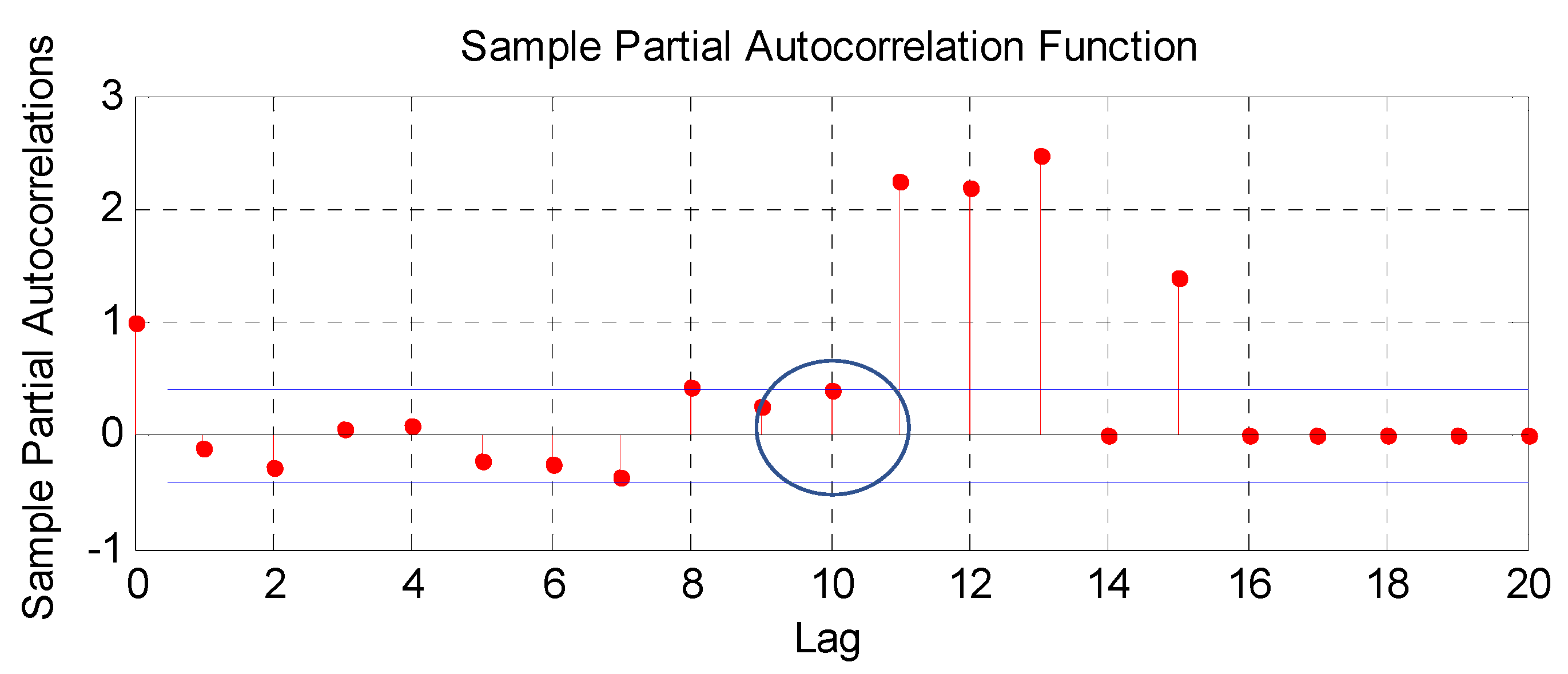
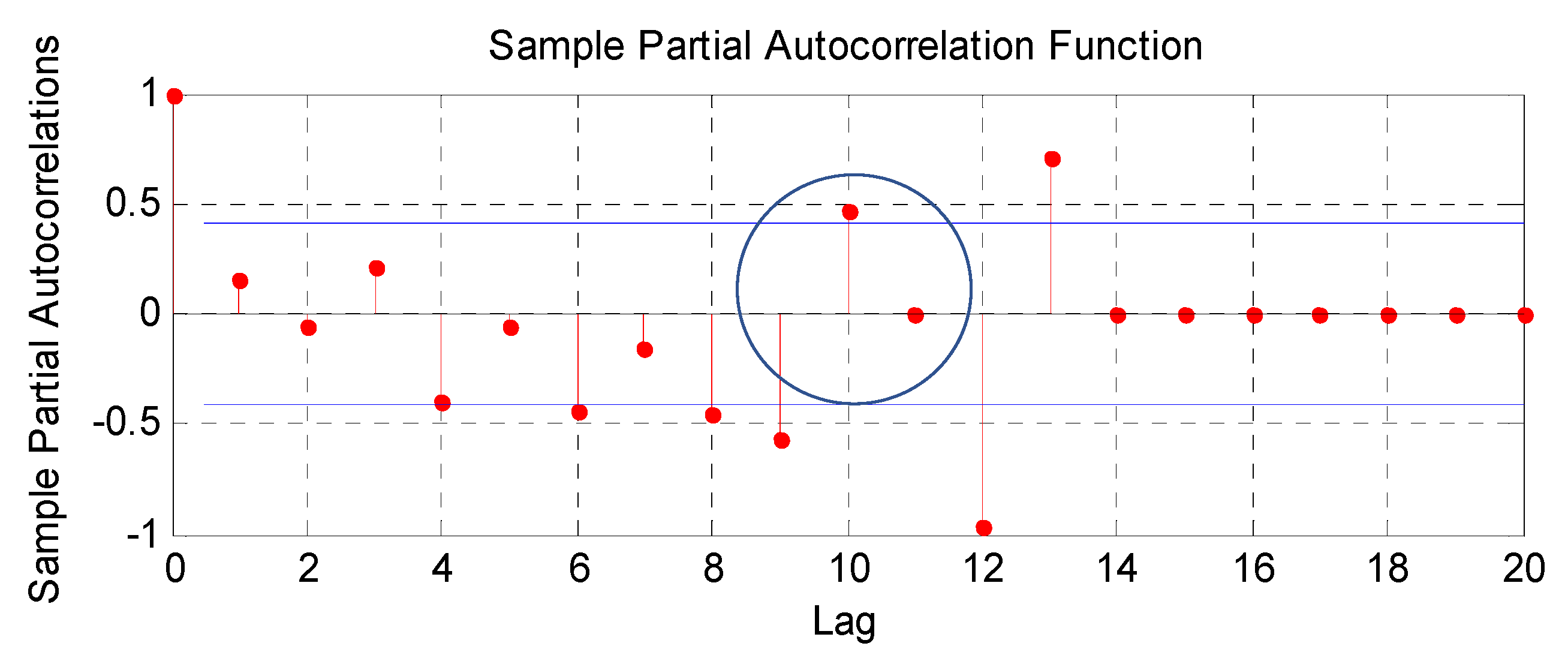
Number of observations is T = 24, so the order of AR process is $\rho \cong \frac{24}{2}-2=10$. Partial autocorrelation function of the previous series is shown in Figure 2.

Figure 2. Partial autocorrelation function of time series composed of 1 and −1 values.

According to the modified approach, we can see that Lag10 can be used as order of AR process, so $\rho =10$. Coefficients ${\beta }_0,{\beta }_1,{\beta }_2,\dots ,{\beta }_{10}$ are presented in Table 3.

Table 3. Coefficients of AR(10) process.

${\mathit{\beta }}_0$	${\mathit{\beta }}_1$	${\mathit{\beta }}_2$	${\mathit{\beta }}_3$	${\mathit{\beta }}_4$	${\mathit{\beta }}_5$	${\mathit{\beta }}_6$	${\mathit{\beta }}_7$	${\mathit{\beta }}_8$	${\mathit{\beta }}_9$	${\mathit{\beta }}_{10}$
−0.3773	−0.0185	0.4000	0.8103	−0.4382	−1.0494	−1.0120	0.0386	0.8052	0.6421	0.4043

Reconstructed (fitted) time series, corresponding states (see Equation (34)), and model accuracy are shown in Table 4.

Table 4. Fitted series with corresponding states and model accuracy.

t	Fitted Value	Fitted State	Original State	Comparison	${\mathit{n}}_{\mathit{t}}^{\mathit{T}\mathit{R}\mathit{U}\mathit{E}}$
11	0.6206	1	1	TRUE	1
12	−1.4927	−1	−1	TRUE	1
13	−0.4918	−1	−1	TRUE	1
14	0.2566	1	1	TRUE	1
15	−1.0000	−1	−1	TRUE	1
16	−0.5794	−1	−1	TRUE	1
17	0.8068	1	1	TRUE	1
18	0.6231	1	−1	FALSE	0
19	0.6360	1	1	TRUE	1
20	0.6927	1	1	TRUE	1
21	−0.1871	−1	1	FALSE	0
22	0.9356	1	1	TRUE	1
23	−0.1922	−1	−1	TRUE	1
24	−0.6283	−1	−1	TRUE	1
Accuracy: 100 × (12/(24 − 10)) = 85.71%				Sum	12

The illustrative example shows that proposed selection of order of autoregressive process can be used to forecast future states of 1 and -1 time series. Applying Equations (33) and (34) beyond T, we obtain forecasted series ${\stackrel{=}{K}}^q\left(t\right),t=T+1,T+2,\dots ,T+h$. Forecasting the displacement for original NN and N state of series is based on Equation (26), where $k_t^q$ and ${\widehat{q}}_t$ are replaced by ${\stackrel{=}{k}}_t^q$ and ${\stackrel{=}{q}}_t,\mathrm{r}\mathrm{e}\mathrm{s}\mathrm{p}\mathrm{e}\mathrm{c}\mathrm{t}\mathrm{i}\mathrm{v}\mathrm{e}\mathrm{l}\mathrm{y}$:

$$∆\stackrel{=}{X}\left(t\right)={\left\{{∆\stackrel{=}{x}}_t\right\}}_{h\times 1}=∆{\stackrel{=}{x}}_{t-1}+{\stackrel{=}{k}}_t^q{\stackrel{=}{q}}_t,t=T+1,T+2,\dots ,T+h$$

(36)

Note that AR($\rho$) model is used only for the forecasting phase, not for prediction (fitting) phase.

For original MD state of series, displacement forecasting is based on the application of Equation (27) beyond T as follows:

$$∆\stackrel{=}{X}\left(t\right)={\left\{{∆\stackrel{=}{x}}_t\right\}}_{h\times 1}={\stackrel{=}{k}}_t\left|∆{\stackrel{=}{x}}_{t-1}+{\stackrel{=}{k}}_t^q{\stackrel{=}{q}}_t\right|,t=T+1,T+2,\dots ,T+h$$

(37)

where $\stackrel{=}{K}\left(t\right)=\left\{{\stackrel{=}{k}}_t\right\},t=T+1,T+2,\dots ,T+h$, is forecasted vector of transformation coefficients for MD state; see Equation (4). Forecasting of the vector $\stackrel{=}{K}\left(t\right)$ is also performed by AR($\rho$), in the same way as we did for series $K^q\left(t\right)$; see Equations (33) and (34). The model of fitting and forecasting the original MD state of series is shown in Table 5.

Table 5. Model of fitting and forecasting the MD state of series.

Fitting Phase *
t	$∆\mathit{X}\left(\mathit{t}\right)$	$\mathit{K}\left(\mathit{t}\right)$ ${\mathit{k}}_{\mathit{t}}\in \left[-\mathrm{1,1}\right]$	$∆\left(∆{\mathit{x}}_{\mathit{t}}\right)$	$\widehat{\mathit{Q}}\left(\mathit{t}\right)$	${\mathit{K}}^{\mathit{q}}\left(\mathit{t}\right)$ ${\mathit{k}}_{\mathit{t}}^{\mathit{q}}\in \left[-\mathrm{1,1}\right]$	$∆\widehat{\mathit{X}}\left(\mathit{t}\right)$	APEt
		Equation (4)	Equation (7)	Equations (19)–(21) and (23)	Equation (25)	Equation (27)	Equation (28)
1	${∆x}_1$	$k_1$
2	${∆x}_2$	$k_2$	$q_1$	$q_1$	$k_1^q$	$k_2\left({∆x}_1+k_1^q{q}_1\right)$	$100\times \left|\frac{{∆x}_2-{∆\widehat{x}}_2}{{∆x}_2}\right|$
3	${∆x}_3$	$k_3$	$q_2$	${\widehat{q}}_2$	$k_2^q$	$k_3\left({∆x}_2+k_2^q{\widehat{q}}_2\right)$	$100\times \left|\frac{{∆x}_3-{∆\widehat{x}}_3}{{∆x}_3}\right|$
4	${∆x}_4$	$k_4$	$q_3$	${\widehat{q}}_3$	$k_3^q$	$k_4\left({∆x}_3+k_3^q{\widehat{q}}_3\right)$	$100\times \left|\frac{{∆x}_4-{∆\widehat{x}}_4}{{∆x}_4}\right|$
⁝	⁝	⁝	⁝	⁝	⁝	⁝	⁝
T − 1	${∆x}_{T-1}$	$k_{T-1}$	$q_{T-2}$	${\hat{q}}_{T-2}$	$k_{T-2}^q$	$k_{T-1}\left({∆x}_{T-2}+k_{T-2}^q{\widehat{q}}_{T-2}\right)$	$100\times \left|\frac{{∆x}_{T-1}-{∆\widehat{x}}_{T-1}}{{∆x}_{T-1}}\right|$
T	${∆x}_T$	kT	$q_{T-1}$	${\widehat{q}}_{T-1}$	$k_{T-1}^q$	$k_T\left({∆x}_{T-1}+k_{T-1}^q{\widehat{q}}_{T-1}\right)$	$100\times \left|\frac{{∆x}_T-{∆\widehat{x}}_T}{{∆x}_T}\right|$
Forecasting Phase *
		$\stackrel{=}{\mathit{K}}\left(\mathit{t}\right)$ ${\stackrel{=}{\mathit{k}}}_{\mathit{t}}\in \left[-\mathrm{1,1}\right]$		$\stackrel{=}{\mathit{Q}}\left(\mathit{t}\right)$	${\stackrel{=}{\mathit{K}}}^{\mathit{q}}\left(\mathit{t}\right)$ ${\stackrel{=}{\mathit{k}}}_{\mathit{t}}^{\mathit{q}}\in \left[-\mathrm{1,1}\right]$	$∆\stackrel{=}{\mathit{X}}\left(\mathit{t}\right)$
		Equations (33) and (34)		Equations (19)–(21) and (23)	Equations (33) and (34)	Equation (37)
T + 1	$∆{\stackrel{=}{x}}_{T+1}$	${\stackrel{=}{k}}_{T+1}$		${\stackrel{=}{q}}_{T+1}$	${\stackrel{=}{k}}_{T+1}^q$	${\stackrel{=}{k}}_{T+1}\left|{∆x}_T+{\stackrel{=}{k}}_{T+1}^q{\stackrel{=}{q}}_{T+1}\right|$
T + 2	${\stackrel{=}{x}}_{T+2}$	${\stackrel{=}{k}}_{T+2}$		${\stackrel{=}{q}}_{T+2}$	${\stackrel{=}{k}}_{T+2}^q$	${\stackrel{=}{k}}_{T+2}\left|∆{\stackrel{=}{x}}_{T+1}+{\stackrel{=}{k}}_{T+2}^q{\stackrel{=}{q}}_{T+2}\right|$
T + 3	${\stackrel{=}{x}}_{T+3}$	${\stackrel{=}{k}}_{T+3}$		${\stackrel{=}{q}}_{T+3}$	${\stackrel{=}{k}}_{T+3}^q$	${\stackrel{=}{k}}_{T+3}\left|∆{\stackrel{=}{x}}_{T+2}+{\stackrel{=}{k}}_{T+3}^q{\stackrel{=}{q}}_{T+3}\right|$
⁝		⁝		⁝	⁝	⁝
T + h	${\stackrel{=}{x}}_{T+h}$	${\stackrel{=}{k}}_{T+h}$		${\stackrel{=}{q}}_{T+h}$	${\stackrel{=}{k}}_{T+h}^q$	${\stackrel{=}{k}}_{T+h}\left|∆{\stackrel{=}{x}}_{T+h-1}+{\stackrel{=}{k}}_{T+h}^q{\stackrel{=}{q}}_{T+h}\right|$

* from t = 1 to t = T—fitting phase; from t = T + 1 to T + h—forecasting phase.

The model of fitting and forecasting the original NN and N state of series is similar, but the AR($\rho$) process of $K\left(t\right),k_t\in \left[-\mathrm{1,1}\right]$ is excluded. In the same way, we model displacement along y-axes.

Finally, according to Equations (1) and (2), we can forecast the changes in the shape of steel arch support as follows:

$$\bigcup _{i=1}^N{\stackrel{=}{M}}_i\left({\stackrel{=}{x}}_i,{\stackrel{=}{y}}_i,t\right),t=T+1,T+2,\dots ,T+h$$

(38)

2.2.3. Model Accuracy Based on Marker Position Error

Accuracy of the fitting model, which is expressed by MAPE, treats displacements along x- and y-axes as two separated time series. However, our problem concerns the fitted position of marker, and it means that we must estimate the closeness between fitted and monitored position of marker. Accordingly, this approach of model accuracy estimation deals with analysis of an error between monitored and fitted position of marker [29,30]. Figure 3 shows the principle used to define the position error.

Figure 3. Error between monitored and fitted position of the marker.

Nomenclature in Figure 3:

• M(x,y)—monitored position of marker
• M(x,y)—fitted position of marker
• ${\overrightarrow{\mathit{R}}}_{\mathit{M}}$—monitored position vector of marker
• ${\mathit{\phi }}_{\mathit{M}}$—angle of monitored position vector with respect to x-axis
• ${\overrightarrow{R}}_M$—fitted position vector of marker
• ${\phi }_M$—angle of fitted position vector with respect to x-axis
• $\overrightarrow{E}$—error vector of fitted position of marker
• ${\phi }_E$—angle error of fitted position vector, ${\mathit{\phi }}_{\mathit{M}}-{\phi }_M$
• $\delta$—angle between fitted position vector and error vector
• $\theta$—angle between error vector and monitored position vector, ${180}^{\mathrm{o}}-\left({\phi }_E+\delta \right)$
• ${\overrightarrow{P}}_M$—the projection of fitted position vector on monitored position vector
• ${\overrightarrow{P}}_E$—the projection of error vector on monitored position vector

The mechanism that we use to estimate fitting error concerns how much a vector is equal to another vector, in the same direction. Desired direction is direction of monitored position vector. Accordingly, we calculate the vector projection of ${\overrightarrow{R}}_M$ on the vector ${\overrightarrow{\mathit{R}}}_{\mathit{M}}$ as follows:

$${\overrightarrow{P}}_M={proj}_{{\overrightarrow{\mathit{R}}}_{\mathit{M}}}{\overrightarrow{R}}_M=\frac{{\overrightarrow{R}}_M·{\overrightarrow{\mathit{R}}}_{\mathit{M}}}{\left|{\overrightarrow{\mathit{R}}}_{\mathit{M}}\right|\left|{\overrightarrow{\mathit{R}}}_{\mathit{M}}\right|}{\overrightarrow{\mathit{R}}}_{\mathit{M}}=P_{M_x}·\overrightarrow{l}+P_{M_y}·\overrightarrow{J}$$

(39)

where $\overrightarrow{l}$ and $\overrightarrow{J}$ are unit vectors along x- and y-axis, respectively. Magnitude of the vector ${\overrightarrow{P}}_M$ equals

$$\left|{\overrightarrow{P}}_M\right|=\sqrt{{\left(P_{M_x}\right)}^2+{\left(P_{M_y}\right)}^2}$$

(40)

Similarly, magnitude of the vector ${\overrightarrow{P}}_E$ is as follows:

$$\left|{\overrightarrow{P}}_E\right|=\sqrt{{\left(P_{E_x}\right)}^2+{\left(P_{E_y}\right)}^2}$$

(41)

Monitored position vector of marker M(x,y) can be presented as a sum of vector ${\overrightarrow{R}}_M$ and vector $\overrightarrow{E}$, i.e., vector ${\overrightarrow{\mathit{R}}}_{\mathit{M}}$ is a resultant of these two vectors:

$${\overrightarrow{\mathit{R}}}_{\mathit{M}}={\overrightarrow{R}}_M+\overrightarrow{E}$$

(42)

Vector ${\overrightarrow{\mathit{R}}}_{\mathit{M}}$ can also be presented as resultant of the following two vectors:

$${\overrightarrow{\mathit{R}}}_{\mathit{M}}={\overrightarrow{P}}_M+{\overrightarrow{P}}_E$$

(43)

Note that the following equality does not hold, according to the triangle inequality:

$$\left|{\overrightarrow{R}}_M\right|+\left|\overrightarrow{E}\right|=\left|{\overrightarrow{P}}_M\right|+\left|{\overrightarrow{P}}_E\right|$$

(44)

In our case (see Figure 4), the triangle inequality is

$$\left|{\overrightarrow{\mathit{R}}}_{\mathit{M}}\right|<\left|{\overrightarrow{R}}_M\right|+\left|\overrightarrow{E}\right|$$

(45)

The projection of error vector on monitored position vector of marker can be calculated from Equation (43) as follows:

$${\overrightarrow{P}}_E={\overrightarrow{\mathit{R}}}_{\mathit{M}}-{\overrightarrow{P}}_M$$

(46)

Vectors ${\overrightarrow{\mathit{R}}}_{\mathit{M}}$, ${\overrightarrow{P}}_M$, ${\overrightarrow{P}}_E$ are collinear, since they lie on the same line, so we can transform Equation (46) from vector to a scalar form in the following way:

$$\left|{\overrightarrow{P}}_E\right|=\left|{\overrightarrow{\mathit{R}}}_{\mathit{M}}\right|-\left|{\overrightarrow{P}}_M\right|$$

(47)

Obviously, Equation (47) presents the absolute error of marker position prediction. Absolute percentage error of fitted position of marker is defined as follows:

$$\mathrm{A}\mathrm{P}\mathrm{E}\left(\left|{\overrightarrow{P}}_E\right|\right)=100\times \frac{\left|\left|{\overrightarrow{\mathit{R}}}_{\mathit{M}}\right|-\left|{\overrightarrow{P}}_M\right|\right|}{\left|{\overrightarrow{\mathit{R}}}_{\mathit{M}}\right|}$$

(48)

Accuracy of the fitting in every point in monitoring time, with respect to marker position, is estimated according to the following equation:

$$\mathrm{A}\mathrm{P}\mathrm{E}\left({\left|{\overrightarrow{P}}_E\right|}_t\right)=100\times \frac{\left|{\left|{\overrightarrow{\mathit{R}}}_{\mathit{M}}\right|}_t-{\left|{\overrightarrow{P}}_M\right|}_t\right|}{{\left|{\overrightarrow{\mathit{R}}}_{\mathit{M}}\right|}_t},t=\mathrm{2,3},\dots ,T$$

(49)

Mean absolute percentage error of marker position is shown below:

$$\mathrm{M}\mathrm{A}\mathrm{P}\mathrm{E}\left({\left|{\overrightarrow{P}}_E\right|}_t\right)=\frac{\sum _{t=2}^T\mathrm{A}\mathrm{P}\mathrm{E}\left({\left|{\overrightarrow{P}}_E\right|}_t\right)}{T-1}$$

(50)

Since we are searching for the changes in the steel arch support shape, then we should define the error of shape prediction. According to Equations (2) and (49), error of predicted (fitted) shape of support can be defined in the following way:

$$\mathrm{M}\mathrm{A}\mathrm{P}\mathrm{E}\left(\bigcup _{i=1}^N{\left|{\overrightarrow{P}}_E\right|}_{t,i}\right)=\frac{\sum _{i=1}^N\sum _{t=2}^T\mathrm{A}\mathrm{P}\mathrm{E}\left({\left|{\overrightarrow{P}}_E\right|}_{t,i}\right)}{N\left(T-1\right)}$$

(51)

3. Numerical Example

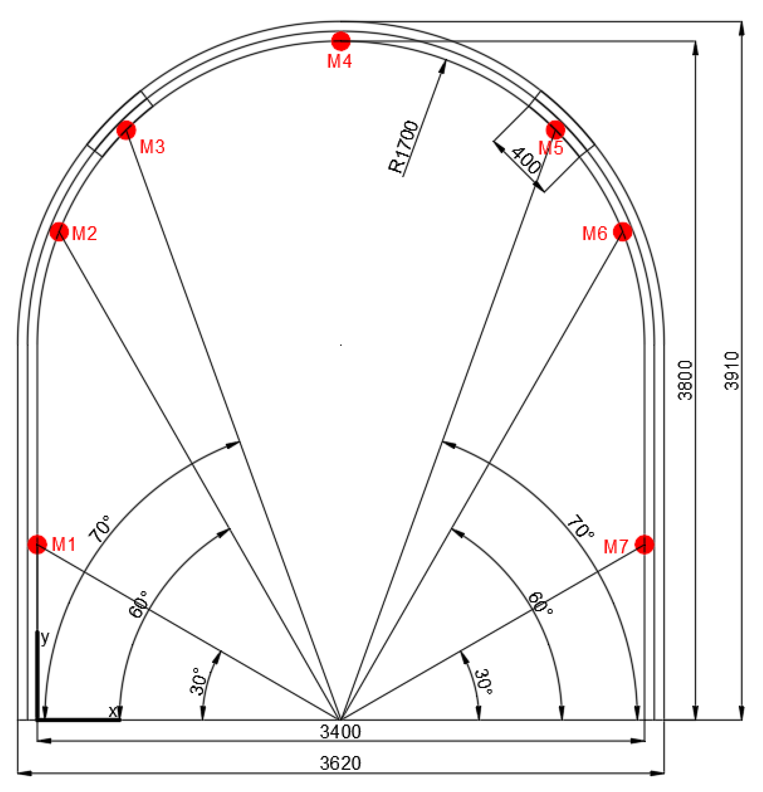
The hypothetical data used in this paper include daily values of displacements of markers along the x- and y-axis, respectively. The period of monitoring is thirty days. This set of displacements is divided into two subsets, fitting and forecasting subsets. The period ranging from the first to the twenty-fifth day (25 values) was used as the fitting subset, and within this interval, we checked the model accuracy by comparing the fitted and monitored values of displacements. The second subset ranging from twenty-six to thirty days (5 values) was used as the validity subset, and in this period, we made a comparison between forecasted and monitored displacements. The positions of seven markers are defined around the internal rim of the steel arch support; see Figure 4.

Figure 4. Steel arch support with positions of the markers.

The coordinates of markers during the monitoring period are presented in Table 6, while the corresponding displacements are shown in Table 7.

Table 6. Monitored coordinates of markers.

MONITORED COORDINATES
Day	M1		M2		M3		M4		M5		M6		M7
	x	y	x	y	x	y	x	y	x	y	x	y	x	y
0	0.0	981.0	122.0	2736.0	498.0	3302.0	1700.0	3800.0	2902.0	3302.0	3278.0	2733.0	3400.0	981.0
1	3.6	977.3	126.0	2732.1	502.3	3297.6	1695.6	3795.2	2897.5	3297.9	3274.0	2728.7	3396.4	977.6
2	7.1	973.5	130.2	2728.1	507.0	3293.4	1691.3	3790.9	2892.9	3293.4	3269.8	2724.9	3392.8	974.0
3	10.6	970.0	134.1	2724.2	511.3	3289.0	1686.6	3786.0	2888.7	3289.2	3265.9	2720.9	3389.3	970.7
4	14.0	966.3	138.1	2720.3	515.8	3284.6	1682.3	3781.4	2884.2	3285.1	3261.8	2717.0	3385.8	967.1
5	17.4	962.6	142.0	2716.2	520.1	3280.2	1677.7	3776.5	2880.0	3280.4	3257.9	2713.3	3382.2	963.6
6	20.8	958.9	146.1	2712.2	524.4	3275.7	1681.9	3772.0	2875.7	3276.1	3254.1	2709.3	3378.8	959.8
7	24.3	955.4	150.2	2707.9	529.0	3271.2	1686.5	3767.4	2871.2	3271.7	3250.3	2705.4	3375.4	956.2
8	27.6	951.6	154.3	2703.8	533.4	3267.1	1682.2	3763.0	2866.9	3267.2	3246.4	2701.5	3371.9	952.7
9	31.1	948.0	158.3	2699.6	537.8	3262.7	1686.7	3758.2	2862.6	3263.2	3242.7	2697.4	3368.3	949.1
10	34.7	944.2	162.4	2695.4	542.2	3258.2	1691.0	3753.4	2858.3	3258.6	3239.0	2693.8	3364.6	945.4
11	38.1	940.3	166.3	2691.4	546.6	3254.1	1686.8	3748.8	2853.8	3254.2	3235.2	2689.8	3361.2	941.7
12	41.7	936.5	170.5	2687.4	551.0	3249.7	1691.4	3744.3	2849.5	3249.9	3231.3	2685.8	3357.7	938.3
13	45.2	932.8	174.6	2683.4	555.1	3245.5	1686.5	3739.7	2845.1	3245.3	3227.4	2681.9	3354.3	934.8
14	48.5	929.2	178.6	2679.2	559.4	3241.1	1682.1	3734.8	2840.7	3241.1	3223.2	2677.9	3350.7	931.1
15	52.0	925.6	182.8	2675.1	563.7	3236.6	1677.4	3729.9	2836.4	3236.6	3219.3	2673.7	3347.1	927.6
16	55.5	921.9	186.5	2671.0	568.3	3232.2	1673.0	3725.0	2832.3	3232.3	3215.6	2669.6	3343.7	924.1
17	59.0	918.1	190.3	2667.3	572.6	3228.0	1677.3	3720.3	2827.9	3227.8	3211.5	2665.6	3340.0	920.5
18	62.5	914.4	194.2	2663.1	577.0	3223.6	1681.5	3715.3	2823.2	3223.3	3207.8	2661.6	3336.3	916.9
19	65.9	910.8	198.3	2659.1	581.4	3219.5	1685.7	3710.2	2818.8	3219.0	3204.1	2657.5	3332.7	913.5
20	69.4	907.2	202.4	2655.2	585.9	3215.2	1690.1	3705.5	2814.5	3214.5	3200.3	2653.6	3329.0	909.8
21	72.9	903.3	206.4	2650.9	590.5	3210.8	1685.6	3700.8	2810.3	3210.3	3196.7	2649.3	3325.4	906.4
22	76.5	899.5	210.6	2646.7	594.6	3206.5	1689.8	3696.0	2806.0	3205.7	3193.0	2645.1	3322.1	902.8
23	79.8	895.7	214.5	2642.6	599.0	3202.0	1694.2	3691.4	2801.4	3201.2	3189.0	2641.2	3318.8	899.2
24	83.2	892.0	218.5	2638.5	603.2	3197.5	1689.9	3686.4	2797.0	3196.6	3184.9	2637.4	3315.4	895.8
25	86.7	888.3	222.4	2634.4	607.7	3192.5	1685.5	3681.8	2792.7	3192.5	3180.8	2633.1	3311.9	892.2
26	90.2	884.6	226.4	2630.6	612.0	3188.4	1681.1	3677.4	2788.5	3188.1	3176.9	2628.9	3308.4	888.6
27	93.8	880.8	230.3	2626.9	616.4	3183.7	1676.3	3672.8	2784.5	3183.7	3173.2	2625.3	3304.9	885.0
28	97.1	877.0	234.4	2623.0	620.9	3179.3	1671.9	3668.0	2780.3	3179.4	3169.3	2621.2	3301.3	881.5
29	100.6	873.3	238.0	2618.9	625.3	3174.6	1667.6	3663.4	2775.9	3175.3	3165.2	2617.1	3297.8	878.1
30	104.3	869.5	241.9	2614.9	629.4	3170.2	1672.0	3658.7	2771.7	3171.2	3161.3	2613.2	3294.2	874.4

Table 7. Displacements of the markers.

DISPLACEMENT
Day	M1		M2		M3		M4		M5		M6		M7
	Δx	Δy	Δx	Δy	Δx	Δy	Δx	Δy	Δx	Δy	Δx	Δy	Δx	Δy
1	3.6	−3.7	4.0	−3.9	4.3	−4.4	−4.4	−4.8	−4.5	−4.1	−4.0	−4.3	−3.6	−3.4
2	3.5	−3.6	4.1	−4.0	4.7	−4.2	−4.3	−4.3	−4.6	−4.4	−4.2	−3.9	−3.7	−3.5
3	3.6	−3.5	4.0	−3.9	4.3	−4.4	−4.7	−4.9	−4.2	−4.3	−3.9	−4.0	−3.5	−3.4
4	3.4	−3.7	4.1	−3.8	4.5	−4.3	−4.3	−4.6	−4.5	−4.1	−4.1	−3.9	−3.4	−3.6
5	3.5	−3.6	3.9	−4.2	4.3	−4.4	−4.6	−4.8	−4.1	−4.6	−3.9	−3.6	−3.6	−3.5
6	3.4	−3.7	4.1	−4.0	4.4	−4.6	4.3	−4.5	−4.3	−4.4	−3.8	−4.0	−3.4	−3.8
7	3.5	−3.5	4.2	−4.4	4.6	−4.4	4.6	−4.6	−4.6	−4.3	−4.0	−3.9	−3.3	−3.6
8	3.2	−3.7	4.1	−4.1	4.4	−4.2	−4.4	−4.4	−4.5	−4.5	−3.9	−4.0	−3.5	−3.5
9	3.5	−3.6	4.0	−4.2	4.5	−4.4	4.5	−4.8	−4.3	−4.1	−3.7	−4.1	−3.6	−3.6
10	3.6	−3.8	4.1	−4.1	4.4	−4.5	4.3	−4.7	−4.4	−4.5	−3.6	−3.6	−3.7	−3.7
11	3.4	−3.9	3.9	−4.0	4.3	−4.2	−4.2	−4.6	−4.5	−4.4	−3.8	−4.0	−3.4	−3.5
12	3.6	−3.8	4.2	−4.1	4.4	−4.3	4.6	−4.5	−4.3	−4.3	−3.9	−4.1	−3.5	−3.4
13	3.5	−3.7	4.1	−4.0	4.1	−4.2	−4.9	−4.6	−4.5	−4.6	−4.1	−3.9	−3.3	−3.6
14	3.4	−3.6	4.0	−4.2	4.4	−4.4	−4.4	−4.9	−4.4	−4.2	−4.2	−4.0	−3.6	−3.7
15	3.5	−3.5	4.2	−4.1	4.3	−4.5	−4.7	−5.0	−4.3	−4.5	−4.0	−4.3	−3.5	−3.5
16	3.6	−3.7	3.7	−4.0	4.5	−4.3	−4.5	−4.8	−4.1	−4.4	−3.7	−4.0	−3.4	−3.6
17	3.4	−3.9	3.8	−3.7	4.4	−4.2	4.4	−4.7	−4.4	−4.5	−4.1	−3.9	−3.7	−3.7
18	3.5	−3.7	4.0	−4.2	4.6	−4.4	4.2	−5.0	−4.6	−4.4	−3.6	−4.0	−3.6	−3.5
19	3.4	−3.6	4.1	−4.0	4.5	−4.1	4.1	−5.1	−4.4	−4.3	−3.7	−4.1	−3.7	−3.4
20	3.5	3.7	4.0	−4.2	4.4	−4.3	4.4	−4.7	−4.3	−4.5	−3.8	−4.0	−3.6	−3.7
21	3.4	−3.9	3.9	−4.3	4.6	−4.4	−4.5	−4.8	−4.2	−4.2	−3.7	−4.3	−3.5	−3.5
22	3.6	−3.8	4.3	−4.2	4.1	−4.3	4.2	−4.7	−4.4	−4.6	−3.9	−4.1	−3.4	−3.6
23	3.2	−3.9	3.9	−4.1	4.4	−4.5	4.4	−4.6	−4.6	−4.4	−4.0	−4.0	−3.3	−3.5
24	3.4	−3.7	4.0	−4.0	4.3	−4.6	−4.3	−5.0	−4.4	−4.6	−4.1	−3.8	−3.4	−3.4
25	3.5	−3.6	3.9	−3.9	4.4	−4.9	−4.4	−4.6	−4.3	−4.1	−4.0	−4.2	−3.6	−3.6
26	3.4	−3.8	4.0	−3.8	4.5	−4.1	−4.6	−4.5	−4.2	−4.4	−3.9	−3.8	−3.4	−3.5
27	3.6	−3.7	3.9	−3.7	4.3	−4.8	−4.8	−4.6	−4.1	−4.5	−3.7	−3.6	−3.5	−3.6
28	3.4	−3.9	4.0	−3.9	4.5	−4.4	−4.4	−4.8	−4.2	−4.3	−3.8	−4.1	−3.6	−3.5
29	3.5	−3.7	3.6	−4.1	4.4	−4.7	−4.2	−4.6	−4.4	−4.2	−4.1	−4.0	−3.5	−3.4
30	3.7	−3.8	3.9	−4.0	4.0	−4.4	4.4	−4.5	−4.2	−4.1	−3.9	−3.9	−3.6	−3.7

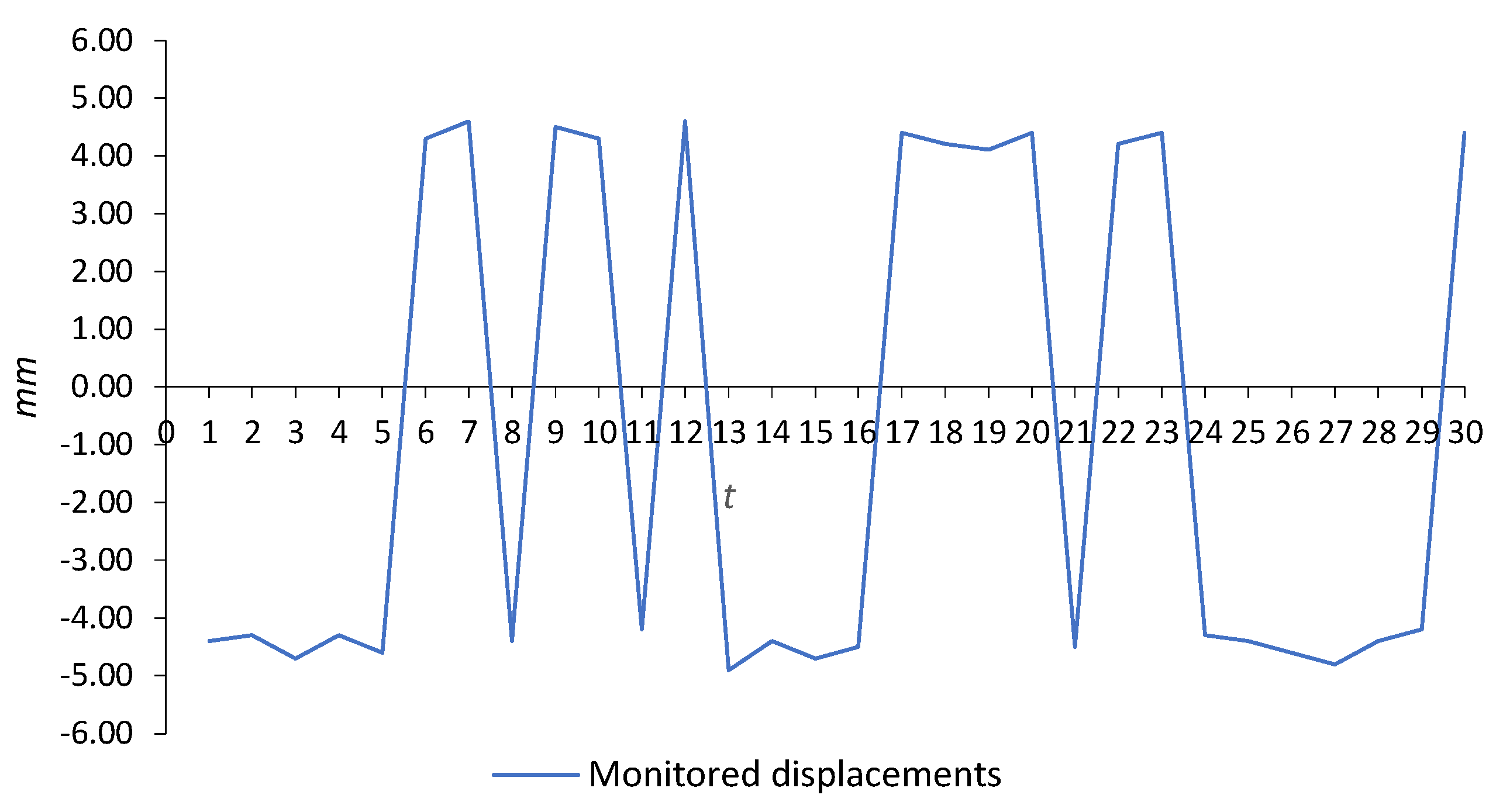
Time series related to displacements of marker M4 along the x-axis was used to show how the model works. Figure 5 presents displacements of marker M4 along the x-axis.

Figure 5. Displacements of the marker M4 along the x-axis.

Despite the randomness in displacement series, there are always some kinds of governing laws. From the previous plot, we can see that the displacement series is too complex and cannot be considered a regular one. According to Equation (3), the series belongs to a mixed time series (MD state). Vector of transformation coefficients for the MD state, and transformation from the MD state to the NN state, are shown in Table 8 and Figure 6.

Table 8. Transformation from MD to NN state of series.

t	1	2	3	4	5	6	7	8	9	10	11	12	13	14	15
MD	−4.4	−4.3	−4.7	−4.3	−4.6	4.3	4.6	−4.4	4.5	4.3	−4.2	4.6	−4.9	−4.4	−4.7
K	−1	−1	−1	−1	−1	1	1	−1	1	1	−1	1	−1	−1	−1
NN	4.4	4.3	4.7	4.3	4.6	4.3	4.6	4.4	4.5	4.3	4.2	4.6	4.9	4.4	4.7
t	16	17	18	19	20	21	22	23	24	25	26	27	28	29	30
MD	−4.5	4.4	4.2	4.1	4.4	−4.5	4.2	4.4	−4.3	−4.4	−4.6	−4.8	−4.4	−4.2	4.4
K	−1	1	1	1	1	−1	1	1	−1	−1	−1	−1	−1	−1	1
NN	4.5	4.4	4.2	4.1	4.4	4.5	4.2	4.4	4.3	4.4	4.6	4.8	4.4	4.2	4.4

Figure 6. Transformation from MD to NN state of series.

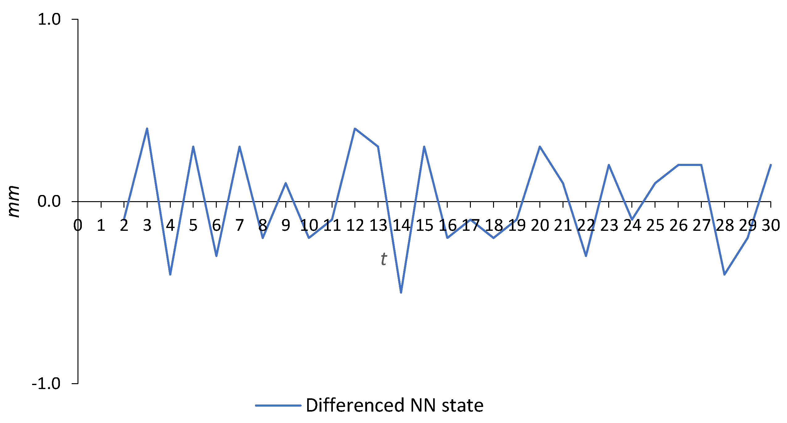
By the first difference of the NN state of the series, we obtain stationary time series, as is shown in Table 9 and Figure 7.

Table 9. First difference of NN state of the series.

t	1	2	3	4	5	6	7	8	9	10	11	12	13	14	15
Diff. NN		−0.1	0.4	−0.4	0.3	−0.3	0.3	−0.2	0.1	−0.2	−0.1	0.4	0.3	−0.5	0.3
t	16	17	18	19	20	21	22	23	24	25	26	27	28	29	30
Diff. NN	−0.2	−0.1	−0.2	−0.1	0.3	0.1	−0.3	0.2	−0.1	0.1	0.2	0.2	−0.4	−0.2	0.2

Figure 7. Stationary series.

Obviously, the stationary time series belongs to the MD state of the series, so we must transform it to the NN state of the series. The way of transformation is presented in Table 10 and Figure 8.

Table 10. Transformation from MD stationary to NN state of series.

t	1	2	3	4	5	6	7	8	9	10	11	12	13	14	15
MD		−0.1	0.4	−0.4	0.3	−0.3	0.3	−0.2	0.1	−0.2	−0.1	0.4	0.3	−0.5	0.3
K		−1	1	−1	1	−1	1	−1	1	−1	−1	1	1	−1	1
NN		0.1	0.4	0.4	0.3	0.3	0.3	0.2	0.1	0.2	0.1	0.4	0.3	0.5	0.3
t	16	17	18	19	20	21	22	23	24	25	26	27	28	29	30
MD	−0.2	−0.1	−0.2	−0.1	0.3	0.1	−0.3	0.2	−0.1	0.1	0.2	0.2	−0.4	−0.2	0.2
K	−1	−1	−1	−1	1	1	−1	1	−1	1	1	1	−1	−1	1
NN	0.2	0.1	0.2	0.1	0.3	0.1	0.3	0.2	0.1	0.1	0.2	0.2	0.4	0.2	0.2

Figure 8. Transformation of stationary MD state of series.

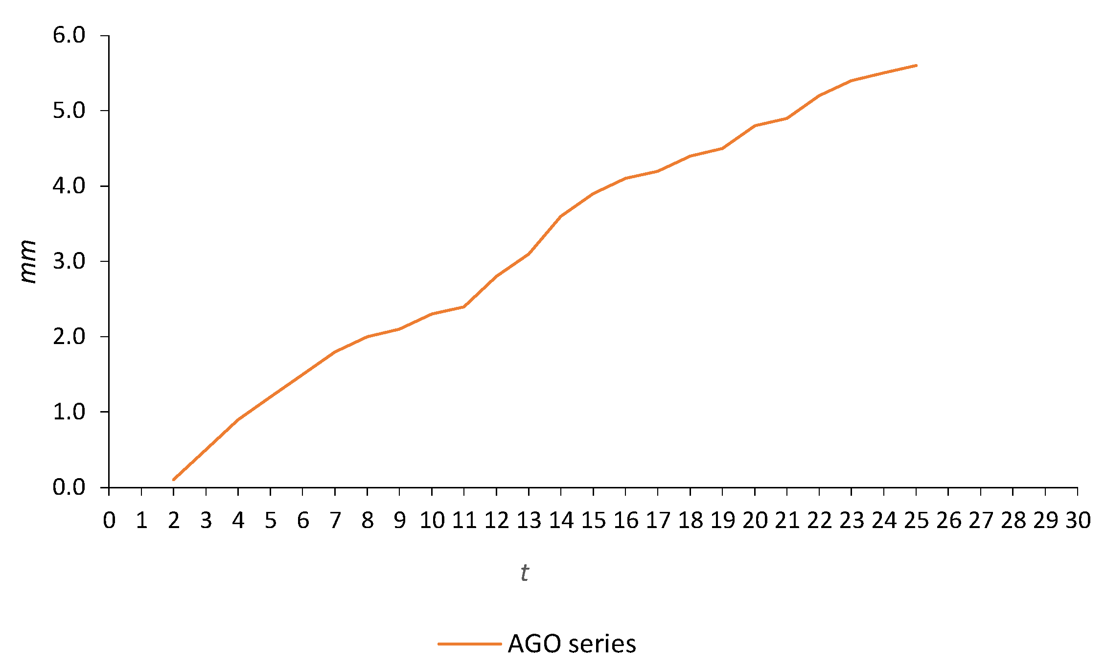
Elements of the transformed stationary series can now be accumulated, and the results of the AGO process are shown in Table 11 and Figure 9. Accumulation is performed only on values from t = 2 to t = 25 (fitting period).

Table 11. AGO series of transformed stationary series.

t	$\mathit{P}\left(\mathit{t}\right)$	${\mathit{P}}^{\left(1\right)}\left(\mathit{t}\right)$	t	$\mathit{P}\left(\mathit{t}\right)$	${\mathit{P}}^{\left(1\right)}\left(\mathit{t}\right)$
1			14	0.5	3.6
2	0.1	0.1	15	0.3	3.9
3	0.4	0.5	16	0.2	4.1
4	0.4	0.9	17	0.1	4.2
5	0.3	1.2	18	0.2	4.4
6	0.3	1.5	19	0.1	4.5
7	0.3	1.8	20	0.3	4.8
8	0.2	2.0	21	0.1	4.9
9	0.1	2.1	22	0.3	5.2
10	0.2	2.3	23	0.2	5.4
11	0.1	2.4	24	0.1	5.5
12	0.4	2.8	25	0.1	5.6
13	0.3	3.1

Figure 9. Accumulated Generation Operation for transformed stationary series (fitting period).

The following matrices are used to calculate parameters a and b of the grey modeling:

$$\mathbf{B}=\left[\begin{array}{cc}-0.30& 1\\ -0.70& 1\\ -1.05& 1\\ -1.35& 1\\ -1.65& 1\\ -1.90& 1\\ -2.05& 1\\ -2.20& 1\\ -2.35& 1\\ -2.60& 1\\ -2.95& 1\\ -3.35& 1\\ -3.75& 1\\ -4.00& 1\\ -4.15& 1\\ -4.30& 1\\ -4.45& 1\\ -4.65& 1\\ -4.85& 1\\ -5.05& 1\\ -5.30& 1\\ -5.45& 1\\ -5.55& 1\end{array}\right],\mathbf{Y}=\left[\begin{array}{c}0.4\\ 0.4\\ 0.3\\ 0.3\\ 0.3\\ 0.2\\ 0.1\\ 0.2\\ 0.1\\ 0.4\\ 0.3\\ 0.5\\ 0.3\\ 0.2\\ 0.1\\ 0.2\\ 0.1\\ 0.3\\ 0.1\\ 0.3\\ 0.2\\ 0.1\\ 0.1\end{array}\right]$$

(52)

According to Equation (12), we obtain a = 0.03454 and b = 0.35021. The parameters of the grey stochastic process are presented in Table 12.

Table 12. Parameters of stochastic AGO series of transformed stationary series.

Parameter	Value
Variance of AGO series $\left({\sigma }^2\right)$	2.88
Time (T)	30 days
Number of steps $\left(\phi \right)$	30
Timestep of $∆t$	1 day
Daily time resolution—coefficient $\left(\omega \right)$	365
Brownian increments—$∆W_t=W_t-W_{t-1}~N\left(0,\frac{{\sigma }^2}{\omega }\right)$	$~N\left(0,\frac{2.88}{365}\right)$

Numerical approximation of $p_t^{\left(1\right)}$ is based on the following Euler–Maruyama discretization:

$$p_t^{\left(1\right)}=p_{t-1}^{\left(1\right)}+\left(0.35021-0.03454·p_{t-1}^{\left(1\right)}\right)·1+N\left(0,\frac{2.88}{365}\right),t=\mathrm{2,3},\dots ,25;p_2^{\left(1\right)}=0.1$$

(53)

Figure 10 shows simulations obtained by Equation (53).

Figure 10. Four simulations of AGO series.

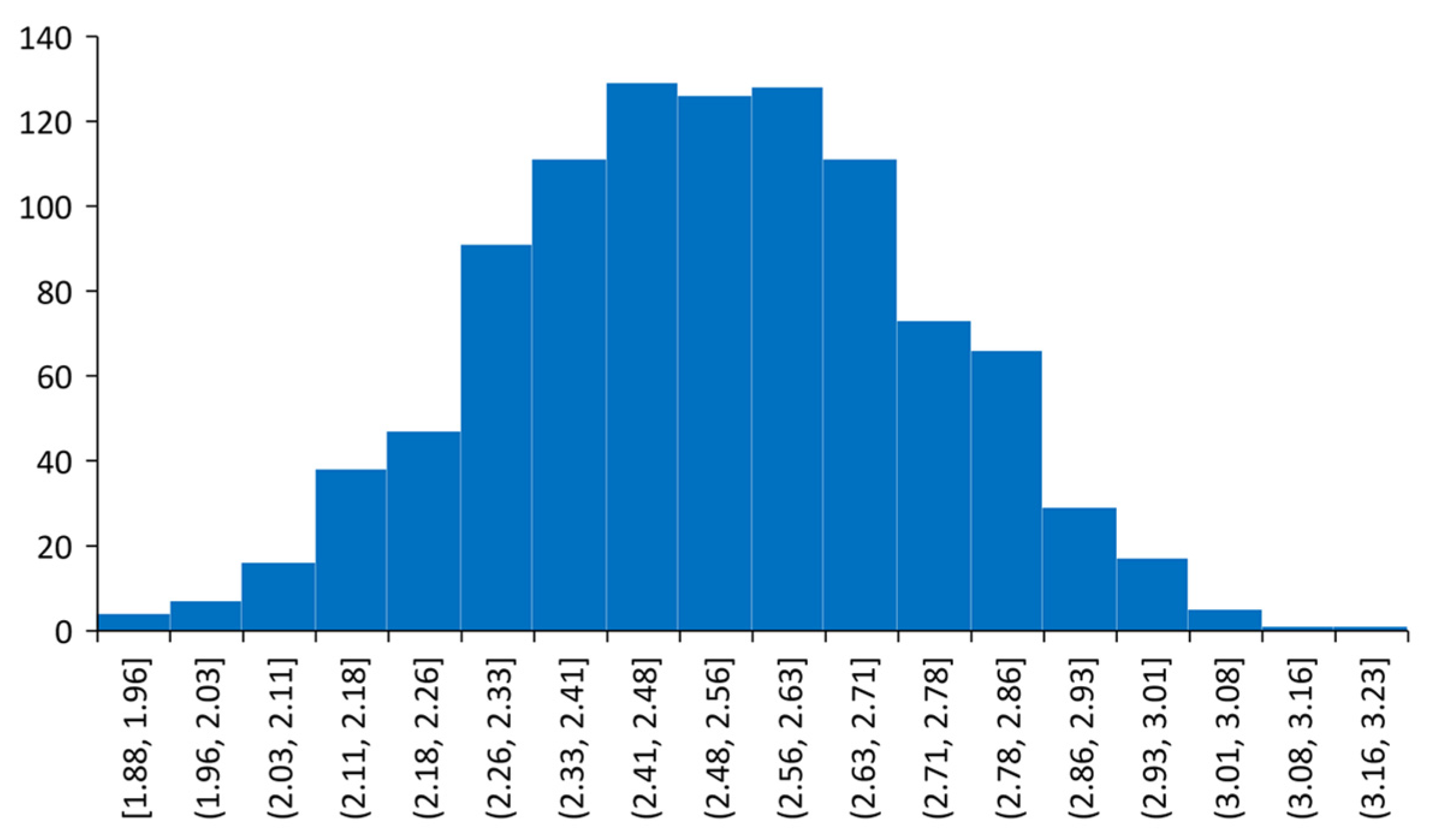
After one thousand simulations of Equation (53), the following expected AGO and corresponding IAGO outcomes are presented in Table 13. Figure 11 presents the probability distribution function of the AGO series for t = 10.

Table 13. Expected AGO and corresponding IAGO outcomes.

t	1	2	3	4	5	6	7	8	9	10	11	12	13	14	15
E(AGO)		0.10	0.44	0.77	1.09	1.40	1.70	1.99	2.27	2.53	2.79	3.04	3.28	3.52	3.74
E(IAGO)		0.10	0.34	0.33	0.32	0.31	0.30	0.29	0.28	0.26	0.26	0.25	0.24	0.23	0.23
t	16	17	18	19	20	21	22	23	24	25	26	27	28	29	30
E(AGO)	3.96	4.17	4.37	4.57	4.75	4.94	5.11	5.28	5.45	5.61
E(IAGO)	0.21	0.21	0.20	0.20	0.19	0.19	0.17	0.17	0.17	0.16

Figure 11. Probability distribution function of AGO series for t = 10 (simulation of Euler–Maruyama equation).

Applying Equation (5) on the expected IAGO outcomes, we obtain the first difference series of displacements for t = 2, 3, …, 25 reconstructed; see Table 14.

Table 14. The first difference series of displacements reconstructed.

t	1	2	3	4	5	6	7	8	9	10	11	12	13	14	15
E(IAGO)		0.10	0.34	0.33	0.32	0.31	0.30	0.29	0.28	0.26	0.26	0.25	0.24	0.23	0.23
K		−1	1	−1	1	−1	1	−1	1	−1	−1	1	1	−1	1
MD		−0.1	0.34	−0.33	0.32	−0.31	0.30	−0.29	0.28	−0.26	−0.26	0.25	0.24	−0.23	0.23
t	16	17	18	19	20	21	22	23	24	25	26	27	28	29	30
E(IAGO)	0.21	0.21	0.20	0.20	0.19	0.19	0.17	0.17	0.17	0.16
K	−1	−1	−1	−1	1	1	−1	1	−1	1
MD	−0.21	−0.21	−0.20	−0.20	0.19	0.19	−0.17	0.17	−0.17	0.16

To obtain the reconstructed (fitted) MD state of the series of displacements, we applied Equation (27), and the results with the corresponding absolute percentage errors are shown in Table 15 and Figure 12.

Table 15. Reconstructed displacements and absolute percentage errors.

t	Original Displacement	Fitted Displacement	APE (%)
1	−4.4
2	−4.3	−4.30
3	−4.7	−4.64	1.32
4	−4.3	−4.37	1.53
5	−4.6	−4.62	0.45
6	4.3	4.29	0.25
7	4.6	4.60	0.01
8	−4.4	−4.31	1.97
9	4.5	4.68	3.94
10	4.3	4.24	1.49
11	−4.2	−4.04	3.85
12	4.6	4.45	3.29
13	−4.9	−4.84	1.23
14	−4.4	−4.67	6.04
15	−4.7	−4.63	1.56
16	−4.5	−4.49	0.32
17	4.4	4.29	2.54
18	4.2	4.20	0.03
19	4.1	4.00	2.33
20	4.4	4.29	2.54
21	−4.5	−4.59	1.90
22	4.2	4.33	3.09
23	4.4	4.37	0.59
24	−4.3	−4.23	1.58
25	−4.4	−4.46	1.40

Figure 12. Original and fitted displacements of marker M4 along x-axis.

The mean absolute percentage error (MAPE) is 1.88%, and according to Table 1, the fitting model of the displacement of marker M4 along the x-axis belongs to a highly accurate class. Fitting errors of displacement for all markers along the x- and y-axis are presented in Table 16.

Table 16. MAPE for all markers during prediction period t = 1, 2, …, 25.

	M1		M2		M3		M4		M5		M6		M7
	x	y	x	y	x	y	x	y	x	y	x	y	x	y
MAPE(%)	2.01	1.28	2.24	2.25	1.92	1.38	1.88	2.54	1.51	2.67	1.95	2.81	1.67	1.64

The MAPE of the model is $1.98\%\approx 2\%$, which points out that the model is capable of forecasting future values of displacement. AGO series beyond T = 25 are forecasted by simulation of Equation (52), for t = 26, 27, 28, 29, 30; and outcomes of expected AGO and corresponding IAGO series are shown in Table 17.

Table 17. Expected AGO and corresponding IAGO outcomes for t = 25, 26, …, 30.

t	1	2	3	4	5	6	7	8	9	10	11	12	13	14	15
E(AGO)		0.10	0.44	0.77	1.09	1.40	1.70	1.99	2.27	2.53	2.79	3.04	3.28	3.52	3.74
E(IAGO)		0.10	0.34	0.33	0.32	0.31	0.30	0.29	0.28	0.26	0.26	0.25	0.24	0.23	0.23
t	16	17	18	19	20	21	22	23	24	25	26 *	27 *	28 *	29 *	30 *
E(AGO)	3.96	4.17	4.37	4.57	4.75	4.94	5.11	5.28	5.45	5.61	5.76	5.90	6.05	6.19	6.32
E(IAGO)	0.21	0.21	0.20	0.20	0.19	0.19	0.17	0.17	0.17	0.16	0.15	0.14	0.15	0.14	0.13

* red color indicates forecasted values.

Application of Equation (5) for the forecasting period requires the transformation coefficient series $K^q\left(t\right)$ to also be forecasted. The two-state time series of the first difference monitored data is presented in Table 18.

Table 18. Two-state time series of marker M4 along x-axis–the first difference, $K^q,t=\mathrm{2,3},\dots ,25$.

1	2	3	4	5	6	7	8	9	10	11	12	13	14	15	16	17	18	19	20	21	22	23	24	25
	−1	1	−1	1	−1	1	−1	1	−1	−1	1	1	−1	1	−1	−1	−1	−1	1	1	−1	1	−1	1

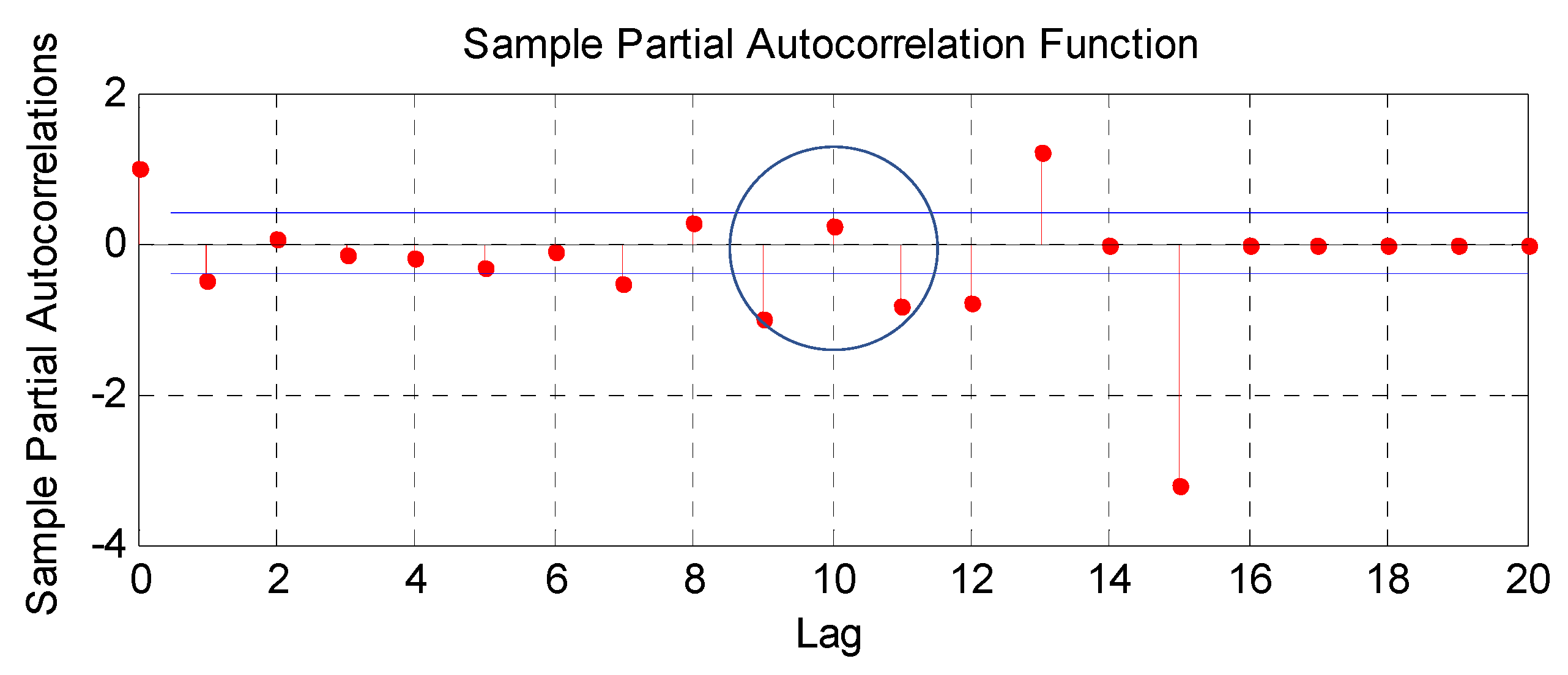
The order of the AR process equals $\rho \cong \frac{24}{2}-2=10$. The plot of the partial autocorrelation function for two-state time series, which is presented in Table 16, is shown in Figure 13. The parameters of the AR(10) process are presented in Table 19.

Figure 13. Partial autocorrelation function of time series composed of 1 and −1 values for first difference displacements (M4x).

Table 19. Coefficients of AR(10) process for M4x–the first difference.

${\mathit{\beta }}_0$	${\mathit{\beta }}_1$	${\mathit{\beta }}_2$	${\mathit{\beta }}_3$	${\mathit{\beta }}_4$	${\mathit{\beta }}_5$	${\mathit{\beta }}_6$	${\mathit{\beta }}_7$	${\mathit{\beta }}_8$	${\mathit{\beta }}_9$	${\mathit{\beta }}_{10}$
−0.3102	0.4298	−0.6724	0.0797	−0.8761	0.1300	−0.3631	−0.4281	−0.1083	−0.9662	0.2305

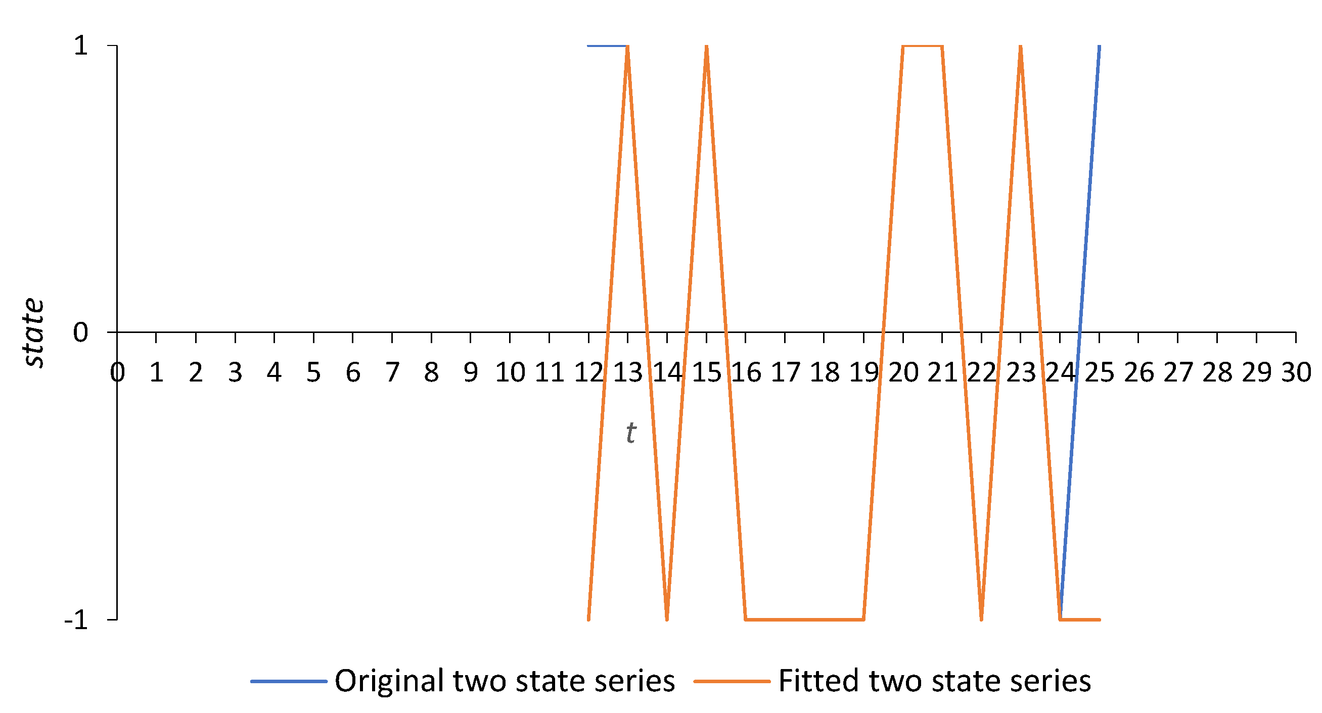
Reconstructed (fitted) time series of M4x, corresponding states (see Equation (34)), and model accuracy are shown in Table 20 and Figure 14. Table 21 shows the accuracy of the AR(10) process for all markers separately.

Table 20. Fitted series with corresponding states, and model accuracy for M4x–the first difference.

t	Fitted Value	Fitted State	Original State	Comparison	${\mathit{n}}_{\mathit{t}}^{\mathit{T}\mathit{R}\mathit{U}\mathit{E}}$
12	−0.1352	−1	1	FALSE	0
13	0.8596	1	1	TRUE	1
14	−0.7799	−1	−1	TRUE	1
15	0.5667	1	1	TRUE	1
16	−1.2877	−1	−1	TRUE	1
17	−0.3588	−1	−1	TRUE	1
18	−0.0052	−1	−1	TRUE	1
19	−0.6395	−1	−1	TRUE	1
20	1.4211	1	1	TRUE	1
21	0.2184	1	1	TRUE	1
22	−0.5789	−1	−1	TRUE	1
23	1.2929	1	1	TRUE	1
24	−0.4315	−1	−1	TRUE	1
25	−0.1421	−1	1	FALSE	0
Accuracy: 100 × (12/(24 − 10)) = 85.71%				Sum	12

Figure 14. Monitored and fitted two-state series for M4x–the first difference.

Table 21. Accuracy of AR(10) model for all markers separately–the first difference.

Two State Series (1 and −1)
Day	M1		M2		M3		M4		M5		M6		M7
	Δx	Δy	Δx	Δy	Δx	Δy	Δx	Δy	Δx	Δy	Δx	Δy	Δx	Δy
12	TRUE	TRUE	TRUE	FALSE	TRUE	TRUE	FALSE	TRUE	TRUE	TRUE	TRUE	TRUE	FALSE	FALSE
13	TRUE	TRUE	TRUE	TRUE	TRUE	TRUE	TRUE	TRUE	FALSE	TRUE	TRUE	TRUE	TRUE	TRUE
14	TRUE	TRUE	TRUE	TRUE	TRUE	TRUE	TRUE	TRUE	TRUE	TRUE	TRUE	TRUE	TRUE	TRUE
15	TRUE	TRUE	TRUE	TRUE	TRUE	TRUE	TRUE	TRUE	TRUE	TRUE	TRUE	TRUE	TRUE	TRUE
16	TRUE	TRUE	TRUE	FALSE	TRUE	TRUE	TRUE	TRUE	FALSE	TRUE	TRUE	TRUE	TRUE	FALSE
17	TRUE	TRUE	TRUE	TRUE	TRUE	TRUE	TRUE	TRUE	TRUE	TRUE	TRUE	TRUE	TRUE	TRUE
18	TRUE	TRUE	TRUE	TRUE	TRUE	TRUE	TRUE	TRUE	TRUE	TRUE	TRUE	TRUE	TRUE	TRUE
19	TRUE	TRUE	FALSE	TRUE	TRUE	TRUE	TRUE	TRUE	TRUE	TRUE	TRUE	FALSE	TRUE	TRUE
20	TRUE	TRUE	TRUE	TRUE	TRUE	TRUE	TRUE	TRUE	TRUE	TRUE	TRUE	TRUE	TRUE	TRUE
21	TRUE	TRUE	TRUE	TRUE	TRUE	TRUE	TRUE	TRUE	TRUE	TRUE	TRUE	TRUE	FALSE	FALSE
22	TRUE	TRUE	TRUE	TRUE	TRUE	TRUE	TRUE	TRUE	TRUE	TRUE	TRUE	TRUE	TRUE	TRUE
23	TRUE	TRUE	TRUE	TRUE	TRUE	TRUE	TRUE	TRUE	TRUE	TRUE	TRUE	TRUE	TRUE	TRUE
24	TRUE	TRUE	TRUE	TRUE	TRUE	TRUE	TRUE	TRUE	FALSE	TRUE	FALSE	TRUE	TRUE	TRUE
25	TRUE	TRUE	TRUE	TRUE	TRUE	TRUE	FALSE	TRUE	TRUE	TRUE	TRUE	TRUE	TRUE	TRUE
AC (%)	100	100	92.86	85.71	100	100	85.71	100	78.57	100	92.86	92.86	85.71	78.57

The expected accuracy of the AR(10) model is 92.34%. Besides the transformation coefficient series $K^q\left(t\right)$ that related to the first difference, the original series of displacements of marker M4 along the x-axis is also related to the transformation coefficient series $K\left(t\right)$; see Table 6 (transformation from the MD to NN state of series). The order of the AR process for series $K\left(t\right)$ equals $\rho \cong \frac{25}{2}-2=10.5$, and we adopt the value of 10. The plot of the partial autocorrelation function for two state time series, which is presented in Table 10, is shown in Figure 15. The parameters of the AR(10) process for the $K\left(t\right)$ series are presented in Table 22.

Figure 15. Partial autocorrelation function of time series composed of 1 and −1 values for original displacements.

Table 22. Coefficients of AR(10) process for M4x-original displacements.

${\mathit{\beta }}_0$	${\mathit{\beta }}_1$	${\mathit{\beta }}_2$	${\mathit{\beta }}_3$	${\mathit{\beta }}_4$	${\mathit{\beta }}_5$	${\mathit{\beta }}_6$	${\mathit{\beta }}_7$	${\mathit{\beta }}_8$	${\mathit{\beta }}_9$	${\mathit{\beta }}_{10}$
−0.0543	0.1103	−0.2452	−0.1739	−0.6446	−0.0214	−0.0548	−0.4679	−0.3268	−0.4487	0.4630

The fitted time series of original displacements of marker M4 along the x-axis, corresponding states (see Equation (34)), and model accuracy are shown in Table 23 and Figure 16.

Table 23. Fitted series with corresponding states, and model accuracy for M4x–original displacements.

t	Fitted Value	Fitted State	Original State	Comparison	${\mathit{n}}_{\mathit{t}}^{\mathit{T}\mathit{R}\mathit{U}\mathit{E}}$
11	0.1540	1	−1	FALSE	0
12	0.7652	1	1	TRUE	1
13	−0.7061	−1	−1	TRUE	1
14	−1.6561	−1	−1	TRUE	1
15	−0.2955	−1	−1	TRUE	1
16	−0.5505	−1	−1	TRUE	1
17	1.0495	1	1	TRUE	1
18	0.3156	1	1	TRUE	1
19	0.5788	1	1	TRUE	1
20	1.4106	1	1	TRUE	1
21	−1.0484	−1	−1	TRUE	1
22	0.5116	1	1	TRUE	1
23	0.1869	1	1	TRUE	1
24	−0.8914	−1	−1	TRUE	1
25	−0.8242	−1	−1	TRUE	1
Accuracy: 100 × (14/(25 − 10)) = 93.33%				Sum	14

Figure 16. Monitored and fitted two state series for M4x–original series.

The accuracy of the model for forecasting two-state series of marker M4x, using the AR(10) process, is presented in Table 24.

Table 24. Forecasted the first difference and monitored two-state series for M4x.

The First Difference					Monitored Values
t	Original State	Forecasted State	Comparison	${\mathit{n}}_{\mathit{t}}^{\mathit{T}\mathit{R}\mathit{U}\mathit{E}}$	Original State	Forecasted State	Comparison	${\mathit{n}}_{\mathit{t}}^{\mathit{T}\mathit{R}\mathit{U}\mathit{E}}$
26	1	1	TRUE	1	−1	−1	TRUE	1
27	1	−1	FALSE	0	−1	−1	TRUE	1
28	−1	−1	TRUE	1	−1	1	FALSE	0
29	−1	−1	TRUE	1	−1	1	FALSE	0
30	1	−1	FALSE	0	1	1	TRUE	1
Accuracy: 100 × (3/5) = 60%					Accuracy: 100 × (3/5) = 60%

We proposed Table 25 to express the accuracy of the AR($\rho$) two-state model in a linguistic way.

Table 25. Linguistic description of model accuracy for two-state series.

Linguistic Description	AC (%)
High accuracy	(75–100]
Good accuracy	(50–75]
Reasonable accuracy	(25–50]
Inaccurate	≤25

The accuracy of the forecasted two-state series for all markers, regarding the first difference, is shown in Table 26.

Table 26. Accuracy of AR(10) model for all markers separately forecasted the first difference.

Two State Series (1 and −1)
Day	M1		M2		M3		M4		M5		M6		M7
	Δx	Δy	Δx	Δy	Δx	Δy	Δx	Δy	Δx	Δy	Δx	Δy	Δx	Δy
26	TRUE	TRUE	FALSE	FALSE	FALSE	TRUE	TRUE	TRUE	TRUE	FALSE	FALSE	FALSE	FALSE	FALSE
27	TRUE	FALSE	TRUE	FALSE	FALSE	FALSE	FALSE	TRUE	FALSE	TRUE	TRUE	TRUE	TRUE	FALSE
28	TRUE	FALSE	FALSE	TRUE	FALSE	TRUE	TRUE	FALSE	TRUE	TRUE	FALSE	FALSE	TRUE	FALSE
29	TRUE	TRUE	FALSE	TRUE	TRUE	TRUE	TRUE	TRUE	TRUE	FALSE	TRUE	TRUE	TRUE	TRUE
30	TRUE	TRUE	TRUE	TRUE	FALSE	TRUE	FALSE	FALSE	TRUE	TRUE	FALSE	TRUE	FALSE	FALSE
AC (%)	100	60	40	60	20	80	60	60	80	60	40	60	60	20

The expected accuracy of the AR(10) model, for the first difference, is 57.14%. According to Table 26, we can conclude the model is classified as good, and can be applied to forecast the first difference two-state series.

Furthermore, outcomes of forecasting beyond t = 25 for displacements of marker M4 along the x-axis are presented in Table 27.

Table 27. Forecasted displacements of marker M4 along x-axis.

t	$∆\mathit{X}\left(\mathit{t}\right)$	$\stackrel{=}{\mathit{K}}\left(\mathit{t}\right)$ ${\stackrel{=}{\mathit{k}}}_{\mathit{t}}\in \left[-\mathrm{1,1}\right]$	$\stackrel{=}{\mathit{Q}}\left(\mathit{t}\right)$	${\stackrel{=}{\mathit{K}}}^{\mathit{q}}\left(\mathit{t}\right)$ ${\stackrel{=}{\mathit{k}}}_{\mathit{t}}^{\mathit{q}}\in \left[-\mathrm{1,1}\right]$	$∆\stackrel{=}{\mathit{X}}\left(\mathit{t}\right)$	Monitored Displacement	APE(%)
AP		Equations (33) and (34)	Equations (19)–(21) and (23)	Equations (33) and (34)	Equation (37)
26	$∆{\stackrel{=}{x}}_{26}$	−1	0.15 *	1	$-1·\left|-4.4+1·0.15\right|=-4.25$	−4.6	7.60
27	$∆{\stackrel{=}{x}}_{27}$	−1	0.14 *	−1	$-1·\left|-4.25-1·0.14\right|=-4.39$	−4.8	8.54
28	$∆{\stackrel{=}{x}}_{28}$	1	0.15 *	−1	$1·\left|-4.39-1·0.15\right|=4.54$	−4.4	203.18
29	$∆{\stackrel{=}{x}}_{29}$	1	0.14 *	−1	$1·\left|4.54-1·0.14\right|=4.40$	−4.2	204.76
30	$∆{\stackrel{=}{x}}_{30}$	1	0.13 *	−1	$1·\left|4.40-1·0.13\right|=4.27$	4.4	2.95

* red color indicates forecasted values.

Mean absolute percentage error equals 85.41%. That is to be expected; if the model gets just one state wrong, then the forecast error increases significantly. Forecasted displacements for all markers and corresponding errors are presented in Table 28.

Table 28. Forecasted displacements for all markers separately.

Day	M1		M2		M3		M4		M5		M6		M7
	Δx	Δy	Δx	Δy	Δx	Δy	Δx	Δy	Δx	Δy	Δx	Δy	Δx	Δy
26	3.33	−3.73	3.68	3.68	4.22	−4.72	−4.25	−4.42	−4.18	−3.83	−4.16	−4.41	−3.73	−3.75
27	3.50	−3.87	3.46	3.46	4.40	−4.53	−4.39	−4.59	−4.29	−4.10	−4.00	−4.20	−3.86	−3.60
28	3.33	−3.73	3.23	3.23	4.22	−4.35	−4.54	−4.43	−4.40	−3.83	−3.84	−3.99	−3.98	−3.75
29	3.50	−3.60	3.47	3.47	4.04	−4.54	4.40	−4.27	−4.51	−4.11	−4.00	−3.78	−3.86	−3.60
30	3.68	−3.73	3.71	3.71	4.22	−4.35	4.27	−4.43	−4.40	−3.84	−4.16	−3.57	−3.74	−3.45
MAPE (%)	1.53	3.04	9.70	9.46	5.71	5.23	85.41	3.80	3.36	8.38	5.05	9.76	8.74	5.39

The MAPE of the forecasting model is 11.75%, and the model belongs to the good accuracy class (see Table 1), even though the error of M4x is 85.41%. Suppose the model got all the states wrong; in that case, the MAPE of M4x is 197.84%, and the MAPE of the forecasting model is 19.78%.

The application of APE to express the efficiency of the model only in the context of a time series is a very rigorous approach, with respect to the environment of forecasting displacements of markers. From a mining engineering point of view, the position forecasting of a marker presents a desired target. Accordingly, the mean absolute percentage error of marker position is a more suitable way to estimate the accuracy of the forecasting model. Table 29 contains coordinates of markers obtained by the model for t = 25, 26, …, 30 (forecasting-validity phase).

Table 29. Forecasted coordinates of markers (forecasting-validity phase).

Two State Series (1 and−1)
Day	M1		M2		M3		M4		M5		M6		M7
	Δx	Δy	Δx	Δy	Δx	Δy	Δx	Δy	Δx	Δy	Δx	Δy	Δx	Δy
26	90.5	885.3	226.3	2631.5	612.4	3187.7	1797.3	3678.0	2788.2	3189.7	3175.8	2628.7	3308.9	888.7
27	94.0	881.4	229.8	2627.3	616.8	3183.2	1792.9	3673.4	2783.9	3185.6	3171.8	2624.5	3305.0	885.0
28	97.3	877.6	233.0	2623.0	621.1	3178.8	1797.4	3669.0	2779.5	3181.7	3168.0	2620.5	3301.0	881.3
29	100.8	874.0	236.5	2618.5	625.1	3174.3	1801.8	3664.7	2775.0	3177.6	3164.0	2616.7	3297.2	877.7
30	104.5	870.3	240.2	2614.2	629.3	3170.0	1806.1	3660.3	2770.6	3173.7	3159.9	2613.1	3293.5	874.2

The comparison of steel arch support between the monitored, fitted, and forecasted shapes is presented in Figure 17.

Figure 17. Steel arch support shape for t = 0, 10, 25, 30 days (monitored, fitted, and forecasted data).

Calculation of model efficiency, which is based on the position error of a marker, is presented in a few successive steps, and we also used marker M4 as an illustrative marker for t = 10:

Step 1: input data:

-

monitored position of marker M4, defined by coordinates, is M(x,y) = (1691.0, 3753.4);

-

fitted position of marker M4, defined by coordinates, is M(x,y) = (1735.7, 3754.0);

-

monitored position vector of marker M4 is ${\overrightarrow{\mathit{R}}}_{\mathit{M}}=1691.0\overrightarrow{l}+3753.4\overrightarrow{J}$;

-

fitted position vector of marker M4 is ${\overrightarrow{R}}_M=1735.7\overrightarrow{l}+3754.0\overrightarrow{J}$.

Step 2: the projection of fitted position vector on monitored position vector

$$\begin{array}{c}{\overrightarrow{P}}_M={proj}_{{\overrightarrow{\mathit{R}}}_{\mathit{M}}}{\overrightarrow{R}}_M=\frac{1691.0·1735.7+3753.4·3754.0}{\sqrt{{1691.0}^2+{3753.4}^2}·\sqrt{{1691.0}^2+{3753.4}^2}}·\left(1691.0,3753.4\right)\\ =1698.8\overrightarrow{l}+3770.6\overrightarrow{J}\end{array}$$

(54)

Step 3: magnitude of the vector ${\overrightarrow{\mathit{R}}}_{\mathit{M}}$ and ${\overrightarrow{P}}_M$

$$\begin{array}{c}\left|{\overrightarrow{\mathit{R}}}_{\mathit{M}}\right|=4116.7\\ \left|{\overrightarrow{P}}_M\right|=4135.6\end{array}$$

(55)

Step 4: Absolute percentage error of marker position

$$\mathrm{A}\mathrm{P}\mathrm{E}\left({\left|{\overrightarrow{P}}_E\right|}_{t=10}\right)=100\times \frac{\left|4116.7-4135.6\right|}{4116.7}=0.459\%$$

(56)

Applying the same calculation on all markers, we obtain the following errors in Table 30.

Table 30. Marker position error.

MAPE (%)
Phase	M1	M2	M3	M4	M5	M6	M7
Fitting	0.064	0.023	0.003	0.677	0.007	0.010	0.010
Forecasting	0.081	0.021	0.013	1.314	0.027	0.031	0.013

The MAPE of the fitting and forecasting model is 0.113% and 0.2143%, respectively.

4. Conclusions

The stability of the underground roadways (headings, galleries, drifts, gate roads, and drives) is crucial for the smooth operation of a mine. When underground roadways are constructed in complex geological conditions and in a weak rock mass, installation of adequate support construction is necessary for the stability maintenance of the roadways in order to provide its functionality during exploitation time. Even then, mostly due to the influence of the dynamic loads from the rock mass, the deformations of the walls and arch of the underground roadways occur. These deformations are also represented in the support construction. Steel arch support is the most used support construction in the headings and gate roads in underground coal mines. As the deformations of the steel arch support cause the shrinking of the cross-section area of the underground roadways, it is important to monitor and forecast the deformations of the sections that can jeopardize the planned work cycle.

In this paper, we presented a forecasting model based on the grey system theory, which observes the deformations of markers placed on a steel arch support. By measuring the coordinates of the marker in a defined period (25 days), data on the position of the marker are obtained, as well as the increment of the deformations along the x- and y-axis each day. Increments of the deformations along the x- and y-axis are observed as two univariate time series, which are later used for the forecasting of the future states of the markers, i.e., the steel arch support.

The previous chapter detailed our model, which gave a MAPE of forecasting of 11.75% in the case when the error was analyzed from a time series point of view. With such an error, the model accuracy is described as good. As the nature of the described problem is such that the position of the marker, i.e., the future position of the underground construction, is of importance to mining engineers, we introduced the analysis of the error of the marker position to evaluate the effectiveness of the model. The MAPE of the forecasting model is 0.2143%, and in that term, the model accuracy is described as high. For the autoregressive model, the proposed window length of $\rho \cong T/2-2$ showed high accuracy (92.34%) for the AR(10) model for fitted data of corresponding states, while it showed reasonable accuracy (57.14%) for the same model for the validity (forecasting) phase. One of the focuses of future research will be the definition of the optimal window length for an autoregressive model to achieve greater accuracy of the model in general. The development of a smart rolling model is also planned to make the model more user-friendly.

This model can be used by mining engineers in underground coal mines for accurate forecasting of the future states of the steel arch support. Using this model, it is possible to plan the maintenance of underground roadways more efficiently, which further results in fewer stoppages in the process of coal production and lower operating costs of the mine.

References

- Wu, Q.; Yan, B.; Zhang, C.; Wang, L.; Ning, G.; Yu, B. Displacement Prediction of Tunnel Surrounding Rock: A Comparison of Support Vector Machine and Artificial Neural Network. Math. Probl. Eng. 2014, 2014, 351496. [Google Scholar] [CrossRef]
- Luo, X.; Gan, W.; Wang, L.; Chen, Y.; Ma, E. A Deep Learning Prediction Model for Structural Deformation Based on Temporal Convolutional Networks. Comput. Intell. Neurosci. 2021, 2021, 829639. [Google Scholar] [CrossRef]
- Luan, Y.; Weng, L.; Ma, Y.; Luan, H. Lake-Bottom Deformation Special Equipment Measurement Methods and Practice of Mining Under Weishan Lake. Electron. J. Geotech. Eng. 2017, 22, 1363–1376. Available online: https://web.archive.org/web/20180427071546id_/http://www.ejge.com/2017/Ppr2017.0110ma.pdf (accessed on 15 December 2022).
- Ma, X.; Xue, Y.; Bai, C.; Liu, H.; Yu, Y. Prediction Model for Deformation Risk Grade of the Soft Rock Tunnel Based on GRA—Extension. IOP Conf. Ser. Earth Environ. Sci. 2020, 440, 052057. [Google Scholar] [CrossRef]
- Rao, J.; Tao, Y.; Xiong, P.; Nie, C.; Peng, H.; Xue, Y.; Xi, Z. Research on the Large Deformation Prediction Model and Supporting Measures of Soft Rock Tunnel. Adv. Civ. Eng. 2020, 2020, 6630546. [Google Scholar] [CrossRef]
- Guo, Y.; Zhao, M.; Deng, Z. Tunnel surrounding rock deformation forecast analysis based on GM and FEM. Electron. J. Geotech. Eng. 2014, 19, 1379–1394. [Google Scholar]
- Han, U.; Choe, C.; Hong, K.; Pak, C. Prediction of Final Displacement of Tunnels in Time-Dependent Rock Mass Based on the Nonequidistant Grey Verhulst Model. Math. Probl. Eng. 2022, 2022, 3241171. [Google Scholar] [CrossRef]
- Xiong, X. Research on Grey System Model and Its Application on Displacement Prediction in Tunnel Surrounding Rock. Open Mech. Eng. J. 2014, 8, 514–518. [Google Scholar] [CrossRef]
- Zhang, L.; Chen, X.; Zhang, Y.; Wu, F.; Chen, F.; Wang, W.; Guo, F. Application of GWO-ELM Model to Prediction of Caojiatuo Landslide Displacement in the Three Gorge Reservoir Area. Water 2020, 12, 1860. [Google Scholar] [CrossRef]
- Wu, L.Z.; Li, S.H.; Huang, R.Q.; Xu, Q. A new grey prediction model and its application to predicting landslide displacement. Appl. Soft Comput. 2020, 95, 106543. [Google Scholar] [CrossRef]
- Li, S.; Wu, N. A new grey prediction model and its application in landslide displacement prediction. Chaos Solitons Fractals 2021, 147, 110969. [Google Scholar] [CrossRef]
- Li, L.; Qiang, Y.; Li, S.; Yang, Z. Research on Slope Deformation Prediction Based on Fractional-Order Calculus Gray Model. Adv. Civ. Eng. 2018, 2018, 9526216. [Google Scholar] [CrossRef]
- Zhang, W.; Xiao, R.; Shi, B.; Zhu, H.; Sun, Y. Forecasting slope deformation field using correlated grey model updated with time correction factor and background value optimization. Eng. Geol. 2019, 260, 105215. [Google Scholar] [CrossRef]
- Crnogorac, L.; Tokalić, R.; Gligorić, Z.; Milutinović, A.; Lutovac, S.; Ganić, A. Gate Road Support Deformation Forecasting Based on Multivariate Singular Spectrum Analysis and Fuzzy Time Series. Energies 2021, 14, 3710. [Google Scholar] [CrossRef]
- Zhu, Z.; Li, H.; Shang, J.; Wang, W.; Liu, J. Research on the mining roadway displacement forecasting based on support vector machine theory. J. Coal Sci. Eng. 2010, 16, 235–239. [Google Scholar] [CrossRef]
- Xie, J.; Xu, J.; Zhu, W. Gray algebraic curve model-based roof separation prediction method for the warning of roof fall accidents. Arab. J. Geosci. 2016, 9, 514. [Google Scholar] [CrossRef]
- Ju-Long, D. Control problems of grey systems. Syst. Control Lett. 1982, 1, 288–294. [Google Scholar] [CrossRef]
- Deng, J. Grey Control Systems; Press of Huazhong University of Science and Technology: Wuhan, China, 1985. [Google Scholar]
- Deng, J. Introduction to Grey system theory. J. Grey Syst. 1989, 1, 1–24. [Google Scholar]
- Liu, S.; Forrest, J.; Yang, Y. A brief introduction to grey systems theory. Grey Syst. Theory Appl. 2012, 2, 89–104. [Google Scholar] [CrossRef]
- Gligorić, Z.; Gligorić, M.; Halilović, D.; Beljić, Č.; Urošević, K. Hybrid Stochastic-Grey Model to Forecast the Behavior of Metal Price in the Mining Industry. Sustainability 2020, 12, 6533. [Google Scholar] [CrossRef]
- Maruyama, G. Continuous Markov processes and stochastic equations. Rendiconti Circolo Mat. Palermo 1955, 4, 48–90. [Google Scholar] [CrossRef]
- Montaño Moreno, J.J.; Palmer Pol, A.; Sesé Abad, A.; Cajal Blasco, B. Using the R-MAPE index as a resistant measure of forecast accuracy. Psicothema 2013, 25, 500–506. [Google Scholar] [PubMed]
- Lewis, C.D. Industrial and Business Forecasting Methods; Butterworth Scientific: London, UK, 1982. [Google Scholar]
- Khan, M.; Poskitt, D. Window Length Selection and Signal-Noise Separation and Reconstruction in Singular Spectrum Analysis. In Monash Econometrics and Business Statistics Working Papers; No 23/11; Monash University, Department of Econometrics and Business Statistics: Melbourne, Australia, 2011. [Google Scholar]
- Wang, R.; Ma, H.; Liu, G.; Zuo, D. Selection of window length for singular spectrum analysis. J. Frankl. Inst. 2015, 352, 1541–1560. [Google Scholar] [CrossRef]
- Hassani, H.; Mahmoudvand, R.; Zokaei, M. Separability and window length in singular spectrum analysis. Comptes Rendus Math. 2011, 349, 987–990. [Google Scholar] [CrossRef]
- Wooldridge, J. Introductory Econometrics: A Modern Approach, 5th ed.; South-Western Cengage Learning: Mason, OH, USA, 2012; pp. 432–433. ISBN 13 978-1-111-53104-1. [Google Scholar]
- Lee, S.; Rizal, S.; Ahn, H. Analysis of the Position Estimation Error of a Local Positioning System utilizing Mobile Anchors. Preprints 2018, 2018100086. [Google Scholar] [CrossRef]
- Zeng, Y.; Tian, W.; Liao, W. Positional error similarity analysis for error compensation of industrial robots. Robot. Comput. Integr. Manuf. 2016, 42, 113–120. [Google Scholar] [CrossRef]
Disclaimer/Publisher’s Note: The statements, opinions and data contained in all publications are solely those of the individual author(s) and contributor(s) and not of MDPI and/or the editor(s). MDPI and/or the editor(s) disclaim responsibility for any injury to people or property resulting from any ideas, methods, instructions or products referred to in the content. |
© 2023 by the authors. Licensee MDPI, Basel, Switzerland. This article is an open access article distributed under the terms and conditions of the Creative Commons Attribution (CC BY) license (https://creativecommons.org/licenses/by/4.0/).