Abstract
In this paper, the formulation to incorporate the used vibration profile, the stress generated by the product’s application, mass, and the resonance frequency is given. After that, based on the vibration output data, the two-parameter Weibull distribution is used to predict the corresponding reliability indices. In the method, the mentioned stress is incorporated as acceleration response (), and by using a dynamic stress factor . In addition, the Weibull parameters are determined based on the generated maximum and minimum principal vibration stress values. In the paper we show the efficiency of the fitted Weibull distribution to predict the reliability indices, by using its Weibull shape and scale parameters, it is always possible to reproduce the principal vibration stress values. Additionally, from the numerical application, we show how to use the Weibull analysis to determine the reliability index for a desired stress or desired cycle value. Finally, we also present the guidelines to apply the proposed method to any vibration fatigue analysis where the (used to determine the and values), and the value are both known.
1. Introduction
In the industry, accelerated vibration tests are used to qualify mechanical products against vibration loads that induce dynamic loads to the product and lead to fatigue damage, specifically due to resonance and natural frequencies [1,2]. Thus, mechanical elements and systems must be designed and validated to support vibration environments. Mechanical components might fail due to yielding, ultimate limit, buckling, and bending [3], where fatigue is commonly the leading failure mode, and it is mainly generated by random vibration. The nature of random vibrations is complex, and it can be represented with a Fourier analysis, where the random motion is presented as a series of sines and cosines waves that are cycling at their own frequency and amplitude [4]. All the series of frequencies occurring at the same time in the mechanical component induce structural resonances, and it is analyzed by using the power spectral density (PSD) [5], which represents the energy in the time signal at different frequencies and load signal [6]. Since random vibration induces variable amplitude loadings, from which, it is difficult to determine or predict the fatigue life [7], then the measuring unit from the PSD is the root mean square (rms). However, because the PSD represents energy (acceleration), then in the vibration analysis is also required to know the equivalence of the acceleration response commonly in gravities (g), to stress units (Psi). For that purpose, we use the dynamic factor [8]. Fortunately, because the random vibration is a random function of time, then it can be analyzed by using a probability density function. Consequently, a vibration stress model is required to translate the stress and stress ranges to the statistical model derived from the stress approach [9]. Within the literature, there are models to quantify fatigue damage and perform fatigue life prediction, such as simple models, mechanical damage models, statistical models, and models that combine mechanical and probabilistic considerations. Here, we employ a methodology to combine random mechanical vibrations and probabilistic considerations by using the Weibull distribution. The efficiency of the Weibull distribution is based on its principle of consistency [10]. Consequently, we are performing the analysis by considering that, when a force is applied to the area of the component, the stress is transmitted to the entire body of the material and the probability of onset of rupture is the same at any point in the body of the material. In the analysis, the shape parameter is a key value that represents the fatigue induced by the vibration load and, it is determined by the maximal and the minimal principal applied stresses values. Additionally, the scale parameter is dependent on the value and on the required product’s, reliability . Additionally, due to random vibration generating variant stress, the steps to determine the reliability for variable stress are given in Section 4.4.
2. General Random Vibration Background
The principal objective of the reliability testing of a mechanical component or system is that it will meet its field operation conditions [11], and laboratory testing has an important role to evaluate product reliability by performing accelerated life testing. In particular, a mechanical fatigue stress test is performed based on the Basquin equation given as [11].
where is the total number of cycles that the component can sustain at a given stress amplitude level and the constant material parameters A and m represent the intercept and the slope of the S–N curve, respectively. Consequently, the mechanical fatigue life estimation can be performed principally by two main groups, crack nucleation and stress/strain material element [12]. In this work, stress analysis is selected. The induced stress is generated by random vibrations. Whereas the behavior of a vibrating system, as is the structural component subjected to an oscillatory excitation force, is led by Equation (2), which represents the equation of motion, which relates the internal forces of the system with the external forces of excitement [13].
In Equation (2), m, c, and k are the mass, damping, and stiffness of the system, that represent its inertial, dissipative, and elastic properties, respectively. F0 is the excitation force applied to the mass. Thereby in mechanical vibrations exist two main types of vibration testing, the deterministic/swept sine and the random one. However, random vibration testing represents an application most realistic, due to the variance of the level of frequencies and amplitude ranges [14]. In random vibration, the fatigue life analysis is according to the time series approach, and frequency PSD load inputs [15]. Thus, in the estimation of fatigue life for a random vibration environment, an analysis of the amplitude distribution and frequency spectrum is usually required [16]. In addition to that, the mechanical component that will be exposed due to its function to random vibration loads must have a defined fatigue or reliability requirement. Thus, the design team establishes a reliability objective based on the fatigue life. Since random vibration is a random function, there is a certain probability that the movement value will be within a certain range of values, which is why it is described in statistical terms. In fatigue life models, the factors involved are load sequence, type of load, overloads, plasticization, and type of material, among others. Additionally, according to [9], for its analysis, we require a probabilistic concept or a physical quantity that is related to the probability of occurrence. Therefore, the measurement of stress, provoked by random vibration lets us determine the probabilities of failure. Generally, the Weibull distribution has been used to perform the probabilistic analysis [17]. Next, the proposed random vibration stress method and its steps are presented.
3. Proposed Random Vibration—Stress Method
3.1. Random Vibration Stress Analysis
Step 1. Collect input data.
From the applied PSD determine the vibration requirements. Based on Equation (3) [18], determine the corresponding sample size to be used in the Weibull analysis.
Step 2. Perform the vibration testing according to the vibration requirements of step 1.
The vibration testing can be performed by using a vibration system, or by simulation.
Step 3. Determine the acceleration response.
Once the vibration testing is completed, the acceleration responses [8] are determined as
where , is the frequency, is the displacement and is the gravity constant.
Step 4. Determine the dynamic factor.
The vibration dynamic factor [3] is calculated as
where K is the stress concentration factor in the component, C is the distance to the neutral axis, is the distance from the fixed point of the component to the point of application of the mass, G is the gravity constant. I is the moment of inertia and is the effective mass, they are given by Equations (6) and (7) [3], respectively.
In Equation (6), from the structural geometry (hollow beam), H and h are the heights, and B and b are the widths. In Equation (7), is the density of the component’s material, L is the length, and m is the mass applied to the component.
Step 5. Determine the vibration stress and the maximum and minimum principal components values.
Once the acceleration response from Equation (4) and the dynamic factor from Equation (5) are known, the vibration stress is calculated by Equation (8) [3].
From the results obtained, take the maximum value as and the minimum value as . The diagram with the steps to determine the vibration stress is shown in Figure 1.
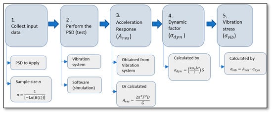
Figure 1.
Diagram overview of the vibration stress calculation.
Now, let us use the above data to perform the corresponding Weibull analysis, based on which the corresponding reliability indices are determined.
3.2. Weibull Statistics Analysis
The two-parameter Weibull distribution is used to analyze statistical fatigue behaviors [10]. It lets us perform accurate fatigue failure analysis [19]. The probability density function and cumulative distribution function are described by Equations (9) and (10), respectively [10].
where is the shape parameter, is the scale parameter, and t is a random variable value that represents the fatigue life. The corresponding reliability function [10] is given as
From [20], the Weibull stress and parameters are determined as
where represents the mean of the Y vector, determined by the median rank approach (See Section 3 [20]). Additionally, [20] represents the log mean of the failure time data, which here is determined directly from the addressed maximum and minimum stresses values of Section 3.1 step 5. Thus is determined as
Here, we note that the efficiency of the Weibull parameters and only depends on the efficiency on which the and values are determined in Section 3.1 step 5. In this paper, they are obtained from an electrodynamic shaker acceleration response once the mechanical component installed in its application system is submitted to a random vibration profile. Once the and values are known, the Weibull stress random analysis is performed as shown in the next section.
3.3. Weibull Stress Random Analysis
Due to the statistical nature of random vibration, the addressed and values are also random. Additionally, because their values are the input to determine the parameters of the associated Weibull distribution, then to determine their random behavior is necessary.
The expected behavior of the and parameters is determined by the following steps:
Step 1. By using the required reliability index in Equation (3), determine the sample size n value. Because in our case = 95% [21], then from Equation (3) n 20.
Step 2. By using the n value from Equation (3) in the median rank approach function stated by Equation (15) [20], the corresponding cumulated failure percentile F(ti) is determined as
Step 3. By using the elements in the linearized form of the reliability function given in Equation (11), determine the corresponding Yi elements as in Equation (16), and then compute its corresponding arithmetic mean value as in Equation (17) [20].
Step 4. By using the value and the and values in Equation (12), determine the corresponding Weibull shape parameter. Similarly, by using the and values in Equation (14), determine the corresponding value, and then by using it in Equation (13), determine the corresponding Weibull scale parameter. These and parameters represent the Weibull stress family that is used to model the random behavior of the estimated principal stresses and values.
Note 1. Here, notice the random behavior of the and values, in the proposed Weibull analysis, let us use the values as the minimum required strength that the component’s material must present, in order to the reliability of the component will be at least (as minimum) the desired index stated in step 1.
From the Weibull analysis, by using the and parameters, the minimum strength values are determined by using the value that corresponds to each element as [20],
Thus, the value is determined as
Additionally, the value is determined as
Additionally, from Equation (21), by using the known value, the [20] element that belongs to the and values determined in Section 3.1 step 5, is determined as
Now, the and the values are used to determine the corresponding [20] value as follows,
Finally, the reliability index that corresponds to the [20] value is determined as
Note 2. Here, observe the index determined in Equation (23) by using the value, according to our proposed method, corresponds to a component with strength equivalent to the value. Thus, if we define the material parameter as the actual strength of the component, then by using this value in Equation (21), and the corresponding value of Equation (22) in Equation (23), the minimum expected reliability of a component that presents a strength of , is determined. Please also notice from the proposed Weibull analysis any desired strength value can be used to determine its corresponding reliability. Now, a numerical application is presented.
4. Numerical Application
The numerical application is performed by using a cable trough straight section, which is shown in Figure 2a. The straight section is a structural component that is used in its field application as a horizontal support for communication cables and it is considered as a hollow straight beam of uniform section and uniformly distributed load. The amount of the cable load and the site environmental vibrations are the principal failure mechanism. The component operational load is 30 Lb. In addition, its relevant data are, length L = 72 in, width W = 4 in, height H = 4 in, and thickness t = 0.125 in. The component is made of thermoplastic ABS with a yield strength = 4350 Psi, ultimate strength = 7250 Psi, and an endurance limit = 3625 Psi [22].
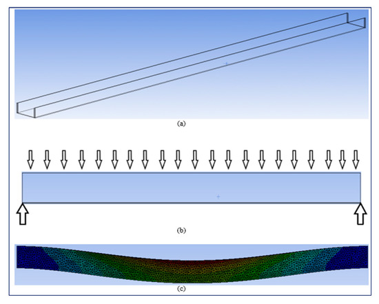
Figure 2.
(a) Cable trough, (b) static load, and (c) static load plus dynamic load applied.
The component has, due to its static functional application, two fixed supports, and a uniform load, see Figure 2b, and due to the dynamic environmental load, it is submitted to random vibration stress, see Figure 2c.
Next, the analysis of the stress induced by the random vibration is performed.
4.1. Random Vibration Stress Analysis
To perform the Weibull stress analysis, it is required to have the principal and stress values. The stress is obtained as follows.
Step1. Random vibration base input PSD.
In this work, the product is regulated by the industrial standard GR-63. It does require that the product resist the random vibration profile PSD shown in Table 1 and Figure 3. It must be applied for 30 s, and it is applied in the three principal axes (x, y, z), respectively.

Table 1.
Random vibration base input profile.
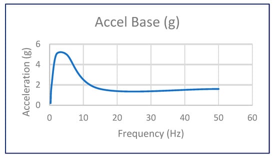
Figure 3.
Acceleration base input.
The sample size is determined by a reliability requirement of 0.95 and by using Equation (3).
Step 2. The vibration base input PSD is applied to the samples by using a shaker machine as shown in Figure 4.
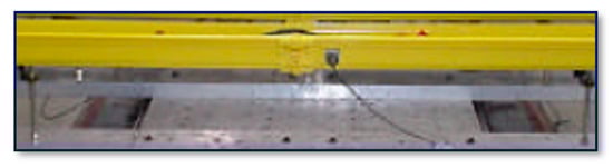
Figure 4.
Component under testing.
Once the vibration base input is applied to the cable trough straight section samples by using a shaker machine, the acceleration response is obtained.
Step 3. The vibration and their acceleration responses are shown in Table 2 and Figure 5. Table 2 is shown the frequencies and their respective accelerations that most affect the cable trough straight sections by each principal axis.
Table 2.
Acceleration response.
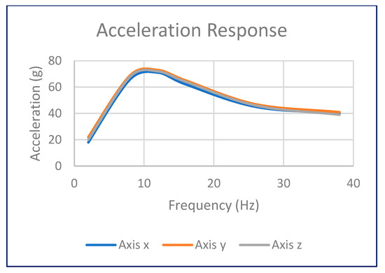
Figure 5.
Acceleration response (three axes).
Step 4. Now, by using Equation (5), the dynamic factor is determined as follows.
The stress concentration factor in the component is, K = 1, since there is no change in the component’s geometry nor holes, the effective mass is, , the distance to the neutral axis is, C = 0.0625 in, the distance from the fixed point of the component to the point of application of the mass is, , the constant gravity is, G and the moment of the inertia . Now, we substitute those values in Equation (5), and the result is, . (See Table 3).
Table 3.
Vibration stress results.
Step 5. Thus, by substituting the acceleration response from step 3 and the dynamic factor from step 4 in Equation (8), the vibration stress induced by the random vibration is obtained, and it is shown in the fourth column in Table 3. The stress values are obtained after the cable trough is exposed to the random vibration in the three principal axes (x, y, z).
From the results of Table 3, the principal vibration stress values = 1188.00 and = 330.00 are obtained. With that data now, we can proceed to use the Weibull distribution with the objective to obtain its reliability and random behavior. Yet, it is required to determine the shape and scale Weibull parameters, respectively.
4.2. Weibull Stress Parameters
By selecting a reliability = 0.95, from Equation (3) we have, , then by using the value in Equation (16), the elements are obtained, with a mean of = −0.544453. Thus, from Equation (12), by using the , , and values, the Weibull parameter value is,
Following the fitting method represented in Section 4. Equation (48) from [20], the constant to be used in Equation (12) from which the Weibull parameters reproduce the observed was determined (see Equation (12)).
In the same way, from Equation (14) the logarithm average value is , and from Equation (13) the Weibull parameter is . Finally, the Weibull stress family is W(1.7087, 626.13 Psi). Now by using the Weibull stress family results, the strength of random behavior can be determined. Since the Weibull parameters only depend on the principal stress values provoked by the random vibration and values, their random behavior can be obtained by performing the Weibull analysis in the following steps.
4.3. Weibull Stress Random Analysis
Since the determination of the fatigue is based on the random behavior of the stress value, here the random behavior of the and are calculated by Equations (19) and (20). Then, by using the and the values in Equation (18), the basic Weibull elements [20] for each are obtained. Whereas using the and values in Equation (21), the Weibull value from the and stresses values are reproduced, it is calculated as,
Additionally, by using the value in Equation (22), the value that belongs to the value is determined as,
Next, by substituting the value in the Equation (23), the reliability that belongs to the element is,
The previous results shown in this section are included in Table 4. Here, it is important to mention that the reliability obtained = 0.716 does not represent the reliability of the design component. The minimal reliability of the component is obtained when the value that belongs to the value is used in Equation (23). The steps to have the reliability of the design component when the value is used as in Equation (21) are, the element that belongs to the value is, . From Equation (22) the corresponding value is, . The reliability index for the value is calculated by using Equation (23), . Thus, we conclude that the reliability of the design component is
Table 4.
Weibull statistics for vibration stress.
The reliability calculated so far is with the condition provided that the component is subjected to constant stress, however, the random vibration that induces the stress, is variant stress. Therefore, for variant stress, the following is stated.
4.4. Material’s Strength for Variant Stress Analysis
In this section the stress–strength analysis is presented due to the component under analysis being submitted to variant stress. In this case, we have the variant vibration forces generated by the principal stresses = 1188 Psi and = 330 Psi. Thus, because the stress now is variant, the index must be determined by performing the corresponding Weibull stress/strength analysis. Since the vibration applied stress and the material strength to support the applied stress, both are random, then, the component’s reliability is determined by a distribution that represents the applied stress and a distribution that represents the strength [23]. Since in this work, the fatigue vibration stress is analyzed by the Weibull distribution, then, the paired combination Weibull–Weibull approach is selected [24,25] and performed by the following relation,
where it is required to determine the stress ƞ and the strength scale parameters. Additionally, the steps to determine the reliability for the used material resistance average , are next.
Step 1. By using the and stresses values in Equation (25), the corresponding mean is,
In addition, from Section 4.2, the corresponding and values are, = 1.7087 and = 626.13 Psi.
Step 2. Determine the strength average of the used material. In this work, the ABS polymeric used material has a .
Step 3. In Equation (26) [20], the and values, the strength scale parameter is,
Then, from Equation (24) with the value = 1.7087, the reliability is,
Thus, the component with a strength of 3625 Psi will have a reliability of , when it is submitted to variant stress (random vibration).
Now, let us present the steps to determine the cycle to failure (N) that corresponds to the random cycles to failure behavior.
4.5. Cycle Random Analysis
In this section, the cycle to failure () value that corresponds to the stress amplitude is determined. The steps are as follows.
Step 1. By using Equation (27) the cycle to failure () value that corresponds to the stress amplitude is determined. Equation (27) according to [11] represents an efficient option to determine the fatigue life.
where the stress amplitude is given by Equation (28) [26]. A and m are given by Equations (29) and (30), respectively.
In Equation (29) a is the fatigue strength coefficient and in Equation (30) b represents the fatigue strength exponent. They are given by Equations (31) and (32), respectively.
The fatigue strength factor f is taken from [26], is the material ultimate stress, and is the material endurance limit.
Now, let us use the data stated in the Section 4 numerical application, starting by substituting the data into Equations (31) and (32) [27], respectively.
The a and b values are included in the Equations (29) and (30), respectively.
The amplitude stress is given by the application of the component submitted to random vibration, where = 1188.00 and = 330.00.
Then, the , A and m values are included in the Equation (27).
This value corresponds to the cycle to failure at the stress amplitude stated.
Step 2. By using the value from Equation (27) and the Weibull element value that corresponds to the stress amplitude value in Equation (21) and Table 4, the corresponding Weibull scale cycle to failure parameter is obtained by Equation (32) [27].
Step 3. The Weibull cycle parameter is employed to determine the corresponding expected cycle to failure values that belongs to each elements in Equation (16). It is performed by using Equation (34) [27].
About the Weibull shape parameter, the value is used in the Weibull cycle to failure family since the failure mode (random vibration) remains constant. Hence, the Weibull cycle to failure family is W (1.7087, 7.700 × 10¹⁶). The corresponding expected cycle to failure values for each one of the elements are determined (see the ninth column in Table 5).
Table 5.
Weibull statistics for cycle to failure analysis.
Finally, as a comparison between the experimental data with the formulation given in Section 3, the principal results are shown in Table 6. From this table, notice that because the addressed Weibull parameters completely reproduce the maximum and minimum vibration stresses, clearly, this Weibull family efficiently lets us predict the reliability indices as it was performed in Table 5.
Table 6.
Experimental and formulation comparison data.
5. Conclusions
- 1.
- The method proposed in this paper allowed us to estimate and predict the fatigue life of cable trough structures based on the stresses fatigue–vibration–Weibull analysis.
- 2.
- The proposed method lets us determine the Weibull parameters directly from the principal vibration stress values obtained after the product’s application, mass, and resonance frequencies were considered in the analysis.
- 3.
- 4.
- The efficiency of the proposed method depends on the accuracy on which the acceleration response and the dynamic factor are determined. This fact is because they determine the principal vibration stress values on which the Weibull parameters are determined.
- 5.
- We highlight that although it seems to be possible to include in the proposed method, the component’s material deformation, because it is based on material properties such as elasticity and ductility, then due to, those material properties affect in the vibration analysis, the acceleration response and dynamic factor, then to generalize the proposed method to the deformation more research must be undertaken.
Author Contributions
Conceptualization, J.M.B.-C., M.R.P.-M. and R.C.T.-V.; methodology, J.M.B.-C. and M.R.P.-M.; data analysis, J.M.B.-C. and R.C.T.-V.; writing—original draft preparation, J.M.B.-C. and M.R.P.-M.; writing—review and editing, J.M.B.-C., M.R.P.-M., and R.C.T.-V.; supervision, M.R.P.-M.; funding acquisition, J.M.B.-C. and R.C.T.-V. All authors have read and agreed to the published version of the manuscript.
Funding
This research received no external funding.
Institutional Review Board Statement
Not applicable.
Informed Consent Statement
Not applicable.
Data Availability Statement
Not applicable.
Conflicts of Interest
The authors declare no conflict of interest.
References
- Mršnik, M.; Slavič, J.; Boltežar, M. Frequency-domain methods for a vibration-fatigue-life estimation—Application to real data. Int. J. Fatigue 2013, 47, 8–17. [Google Scholar] [CrossRef]
- Jang, J.; Park, J.-W. Simplified Vibration PSD Synthesis Method for MIL-STD-810. Appl. Sci. 2020, 10, 458. [Google Scholar] [CrossRef]
- Irvine, T. A Fatigue Damage Spectrum Method for Comparing Power Spectral Density Base Input Specifications. Vibrationdata. 2014. Available online: https://vibrationdata.wordpress.com/ (accessed on 8 March 2023).
- Kumar, S.M. Analyzing Random Vibration Fatigue. Available online: https://ansys.com/ (accessed on 6 March 2023).
- Kong, Y.; Abdullah, S.; Schramm, D.; Omar, M.; Haris, S. Vibration Fatigue Analysis of Carbon Steel Coil Spring under Various Road Excitations. Metals 2018, 8, 617. [Google Scholar] [CrossRef]
- Lalanne, C. Fatigue Damage, 3rd ed.; John Wiley & Sons, Inc.: Hoboken, NJ, USA, 2014; Volume 4. [Google Scholar]
- Gao, H.; Huang, H.-Z.; Zhu, S.-P.; Li, Y.-F.; Yuan, R. A Modified Nonlinear Damage Accumulation Model for Fatigue Life Prediction Considering Load Interaction Effects. Sci. World J. 2014, 2014, 164378. [Google Scholar] [CrossRef] [PubMed]
- Barraza-Contreras, J.M.; Piña-Monarrez, M.R.; Molina, A.; Torres-Villaseñor, R.C. Random Vibration Fatigue Analysis Using a Nonlinear Cumulative Damage Model. Appl. Sci. 2022, 12, 4310. [Google Scholar] [CrossRef]
- Castillo, E.; Fernández-Canteli, A. A Unified Statistical Methodology for Modeling Fatigue Damage; Springer: Berlin/Heidelberg, Germany, 2009. [Google Scholar]
- Weibull, W. A Statistical Theory of the Strength of Materials; Generalstabens Litografiska Anstalts Förlag: Stockholm, Sweden, 1939. [Google Scholar]
- Lee, Y.-L.; Pan, J.; Hathaway, R.B.; Barkey, M.E. Fatigue Testing and Analysis: Theory and Practice; Elsevier Butter-worth-Heinemann: Burlington, MA, USA, 2005. [Google Scholar]
- Santecchia, E.; Hamouda, A.M.S.; Musharavati, F.; Zalnezhad, E.; Cabibbo, M.; El Mehtedi, M.; Spigarelli, S. A Review on Fatigue Life Prediction Methods for Metals. Adv. Mater. Sci. Eng. 2016, 2016, 9573524. [Google Scholar] [CrossRef]
- Gutierrez-Wing, E.S.; Bedolla-Hernández, J.; Vélez-Castán, G.; Cortés-García, C.; Szwedowicz-Wasik, D. Identification of Close Vibration Modes of a Quasi-Axisymmetric Structure: Complementary Study. Ing. Investig. Y Tecnol. 2013, 14, 207–222. [Google Scholar]
- White, P.G. Introducción al Análisis de Vibraciones; AzimaDLI: Woburn, MA, USA, 2010. Available online: https//AzimaDLI.com/ (accessed on 26 February 2023).
- Quigley, J.P.; Lee, Y.-L.; Wang, L. Review and Assessment of Frequency-Based Fatigue Damage Models. SAE Int. J. Mater. Manuf. 2016, 9, 565–577. [Google Scholar] [CrossRef]
- Harris, C.M.; Piersol, A.G. Shock and Vibration Handbook, 5th ed.; McGraw Hill: New York, NY, USA, 2002; Volume 15. [Google Scholar]
- Lindquist, E.S. Strength of materials and the Weibull distribution. Probabilistic Eng. Mech. 1994, 9, 191–194. [Google Scholar] [CrossRef]
- Monarrez, M.R.P.; Ramos-Lopez, M.L.; Alvarado-Iniesta, A.; Molina-Arredondo, R.D. Robust sample siza for Weibull demostartion test plan. Dyna 2016, 83, 52–57. [Google Scholar] [CrossRef]
- Jian, J.; Luo, H.; Li, T.; Zhang, G.; Cui, X. Fatigue life assessment of electromagnetic riveted carbon fiber reinforce plastic/aluminum alloy lap joints using Weibull distribution. In Proceedings of the 24th International Conference Engineering Mechanics, Svratka, Czech Republic, 14–17 May 2018; pp. 41–44. [Google Scholar] [CrossRef]
- Piña-Monarrez, M.R. Weibull stress distribution for static mechanical stress and its stress/strength analysis. Qual. Reliab. Eng. Int. 2017, 34, 229–244. [Google Scholar] [CrossRef]
- Berghmans, F.; Eve, S.; Held, M. An Introduction to Reliability of Optical Components and Fiber Optic Sensors. In NATO Science for Peace and Security Series B: Physics and Biophysics; Springer: Dordrecht, The Netherlands, 2007; pp. 73–100. [Google Scholar] [CrossRef]
- Frascio, M.; Avalle, M.; Monti, M. Fatigue strength of plastics components made in additive manufacturing: First experimental results. Procedia Struct. Integr. 2018, 12, 32–43. [Google Scholar] [CrossRef]
- Boehm, F.; Lewis, E. A stress-strength interference approach to reliability analysis of ceramics: Part I—fast fracture. Probabilistic Eng. Mech. 1992, 7, 1–8. [Google Scholar] [CrossRef]
- Filho, R.L.M.S.; Droguett, E.L.; Lins, I.D.; Moura, M.C.; Amiri, M.; Azevedo, R.V. Stress-Strength Reliability Analysis with Extreme Values based on q-Exponential Distribution. Qual. Reliab. Eng. Int. 2016, 33, 457–477. [Google Scholar] [CrossRef]
- Tijerina, M.B.; Monarrez, M.R.P.; Contrera, J.B. Weibull strength distribution and reliability S-N percentiles for tensile tests. Rev. De Cienc. Tecnológicas 2022, 5, 284–299. [Google Scholar] [CrossRef]
- Budynas, R.; Nisbett, J. Shigley’s Mechanical Engineering Design, 10th ed.; McGraw Hill: New York, NY, USA, 2015. [Google Scholar]
- Barraza-Contreras, J.M.; Piña-Monarrez, M.R.; Molina, A. Fatigue-Life Prediction of Mechanical Element by Using the Weibull Distribution. Appl. Sci. 2020, 10, 6384. [Google Scholar] [CrossRef]


Disclaimer/Publisher’s Note: The statements, opinions and data contained in all publications are solely those of the individual author(s) and contributor(s) and not of MDPI and/or the editor(s). MDPI and/or the editor(s) disclaim responsibility for any injury to people or property resulting from any ideas, methods, instructions or products referred to in the content. |
© 2023 by the authors. Licensee MDPI, Basel, Switzerland. This article is an open access article distributed under the terms and conditions of the Creative Commons Attribution (CC BY) license (https://creativecommons.org/licenses/by/4.0/).