A Mixed Clustering Approach for Real-Time Anomaly Detection

Abstract

Anomaly detection in real-time data is accepted as a vital area of research. Clustering techniques have effectively been applied for the detection of anomalies several times. As the datasets are real time, the time of data generation is important. Most of the existing clustering-based methods either follow a partitioning or a hierarchical approach without addressing time attributes of the dataset distinctly. In this article, a mixed clustering approach is introduced for this purpose, which also takes time attributes into consideration. It is a two-phase method that first follows a partitioning approach, then an agglomerative hierarchical approach. The dataset can have mixed attributes. In phase one, a unified metric is used that is defined based on mixed attributes. The same metric is also used for merging similar clusters in phase two. Tracking of the time stamp associated with each data instance is conducted simultaneously, producing clusters with different lifetimes in phase one. Then, in phase two, the similar clusters are merged along with their lifetimes. While merging the similar clusters, the lifetimes of the corresponding clusters with overlapping cores are merged using superimposition operation, producing a fuzzy time interval. This way, each cluster will have an associated fuzzy lifetime. The data instances either belonging to sparse clusters, not belonging to any of the clusters or falling in the fuzzy lifetimes with low membership values can be treated as anomalies. The efficacy of the algorithms can be established using both complexity analysis as well as experimental studies. The experimental results with a real world dataset and a synthetic dataset show that the proposed algorithm can detect the anomalies with 90% and 98% accuracy, respectively.

1. Introduction

The widespread use of computers, databases and associated networks makes them vulnerable to attacks. Attacks in the form of hacking or intruding are malicious activities that undermine the integrity or security of systems or their resources. The term “anomalous activity” is used for this and any ata instances associated with such activity is named an anomaly. An anomaly is a data object [1] that deviates from those previously observed. Detection of anomalies is now a hot topic of modern research.

Intrusion detection systems (IDS) are security tools that support the safety, security and strength of information and communication systems [2]. Recently, anomaly based IDS have been gaining popularity receiving extensive use because of their ability to detect insider attacks and previously unknown attacks. There are several approaches to developing IDS, and one such approach is data mining.

Data mining is an iterative and interactive process of finding patterns, associations, correlations, variations, anomalies and similar statistically noteworthy structures from large datasets [3]. There are three fundamental practices of data mining, namely unsupervised, supervised and semi-supervised learning [4]. Clustering [5] is an unsupervised learning practice frequently exercised to unearth patterns and the distribution of data. While it has been widely used in social science and psychology, it has also been applied in anomaly detection recently. There are several algorithms developed for this purpose, namely k-means, ROCK, CACTUS, DBSCAN and hierarchical agglomerative algorithms [5,6,7].

Another two important classes of clustering approaches are static clustering and dynamic clustering. Static clustering mostly deals with static datasets that are ready before the use of the algorithm. However, some applications such as wireless sensor networks, IoT, cloud computing, finance and stock markets, where data are real time, demand dynamic clustering. In [8], the authors proposed a hierarchical algorithm that can be used for both static as well as dynamic datasets. In [9], the authors proposed several incremental clustering algorithms that can process new records or data instances as they are added to the dataset. In [10], the authors employed the Elzaki disintegration strategy for solving non-linear equations of Emden–Fowler models. In [11], a fractional order was used for the glioblastoma multiform (GBM) and IS interaction models.

As mentioned earlier, clustering has been widely employed in many areas of anomaly detection. In [12], an algorithm was proposed, which can detect anomalies from datasets with mixed attributes. Using distance and dissimilarity functions, a fuzzy c-means-based clustering method was discussed in [13], which works nicely on both numeric and categorical attributes. In [14], an approach for anomaly detection of a mixed-attribute-dataset was proposed, which adopts both partitioning and hierarchical approaches. Although most of the above-mentioned works were on static datasets, a few addressed the dynamicity of datasets. Anomaly detection from real-time data is interesting and has caught the attention of many researchers. In [15], the authors proposed an anomaly detection technique for the aforesaid data, which can be applicable to both multi-dimensional as well as categorical data. Similar works were presented in [16,17,18]. Since the data generated by real-time systems are real time, there is a need to detect the anomalies at the time of the data generation.

Problems similar to the above have been addressed by different researchers. In [19], the authors proposed an anomaly detection method that includes components based on entropy analysis, signature analysis and machine learning using fractal and recurrence analysis. Yanqin et al. [20] proposed a fuzzy aggregation approach to design an efficient IDS to be deployed in an enterprise gateway. In [21], the authors conducted a comparative study of five-time series anomaly detection models: InterFusion, RANSynCoder, GDN, LSTM-ED and USAD. In [22], the authors introduced a neighborhood rough-set-based classification approach for the anomaly detection of mixed data. Similar works were reported in [23,24,25,26,27].

In [28], the authors introduced a time-series data cube as a new data structure in handling multi-dimensional data for anomaly detection. Gupta et al. [29] conducted a detailed study on anomaly detection of strictly temporal data for both discrete and continuous cases. In [30], the authors presented a classification-based method of online detection of anomalies from highly unreliable data. In [31], an efficient online anomaly detection algorithm for data streams was proposed, which takes into consideration the temporal proximity of the data instances. In [32], the authors provided a foundational framework for cyber risk assessment for operational technology (OT) systems. In [33], the authors proposed how to address the insider threat posing significant cyber security challenges in industrial control systems. Zhao et al. [34] introduced a random forest-based approach for online anomaly detection. In [35,36,37], the authors proposed fuzzy based methods for real-time anomaly detections. In [38], the authors proposed a fuzzy neural network method for anomaly detection in large-scale cyberattacks. In [39], the authors proposed an efficient clustering-based real-time anomaly detection algorithm and demonstrated the efficacy of their algorithm when tested against some well-known algorithms using the datasets: DARPA, MACCDC and DEFCON. Most of the aforesaid methods have handled the time attribute associated with the dataset like any other attribute. However, considering the time attribute separately, interesting time-dependent clusters can be generated.

In this article, a clustering-based anomaly detection algorithm is proposed for real-time data with mixed attributes. The algorithm follows both a partitioning and an agglomerative hierarchical approach and each cluster produced by the algorithm will have an associated fuzzy time interval as its lifetime. The algorithm starts with a partitioning approach then follows an agglomerative hierarchical approach. As the datasets are real time such as data stream, the time of generation (time-stamp) of every data instance is important and the algorithm also takes this into account. The objective of this article is as follows.

• First of all, the data instance–cluster distance measure [7,14] is defined in terms of both numeric and categorical attribute–cluster distance.
• Secondly, the similarity measure of a pair of clusters is expressed in an equivalent manner and a merge function is defined in terms of it.
• Finally, a two-phase method for anomaly detection is proposed.

In the phase one, the first k-data instances are kept in k-different clusters along with their time stamps (time of generation) as cluster creation times or start time of the lifetimes. If a new data instance comes to any of the k-clusters, the lifetime of the cluster is extended by the current time stamp (the time-stamp associated with the data instance). Then, the cluster’s categorical attribute’s frequency and the mean of numeric values are updated. At the end of phase one, each cluster is having an associated lifetime. Then, the agglomerative hierarchical approach starts. In this phase, a merge function based on similarity measure is applied to merge two highly similar clusters if their lifetimes overlap. Then the overlapping lifetimes are kept in a compact form using a set superimposition [40,41]. At any stage of merging, two superimposed intervals associated with two clusters are superimposed based on the non-empty intersection of their cores. Consequently, each resulting cluster will have an associated superimposed time interval, which produces a fuzzy time interval [42,43]. The algorithm stops when no further merger is possible. The algorithm supplies a set of clusters where each cluster will have an associated fuzzy time interval as its lifetime. One of the most challenging issues of partitioning clustering approach is to specify the value of k and there are several methods developed for this purpose. The proposed algorithm has addressed this issue very nicely by producing the same number of stable clusters irrespective of the number of input clusters (k) because the number of clusters will be reduced during the merging phase. Clearly, the number of output cluster will be less than or equal to k, and the output cluster set is more stable and invariant with respect to the number of input cluster. The data instances, which either belong to sparse clusters or does not belong to any of the clusters or fall in the fuzzy lifetimes with very low membership values will be considered as anomalies. Thus, whether a data instance can be an anomaly or not also depends on its time of occurrence or generation. Then the proposed algorithm’s time complexity is evaluated. Finally, an exhaustive evaluation with two datasets, KDDCup’99 Network anomaly dataset [44] and Kitsune Network Attack dataset [45] has been performed along with a comparative analysis against some of the well-known clustering-based approaches of both static and dynamic nature. The results decently demonstrate the efficacy of the proposed algorithm.

The article is arranged as follows. The recent developments in this area are discussed in Section 2. In Section 3, the terms, notations and definitions that have been used here are discussed. In Section 4, the proposed system using algorithm and flowchart is explained. The complexity analysis is given in Section 5. The experimental analysis and the results are given in Section 6. Finally, the paper is winded-up with Conclusions, Limitations and lines for future works in Section 7.

2. Related Works

Anomaly detection is the finding of the data object, which deviates from the previously observed one. In [1], the authors discussed anomalies and different clustering-based techniques and algorithm to identify them. Intrusion detection systems (IDS) are protection steps that can assure safety and security from unauthorized access. There are several well-known IDS available and signature detections system is one of them. Recently, the anomaly based IDS [2] have been gaining popularity because of their wide-spread use and ability to detect insider attacks or previously unknown attacks. Most of the anomaly based IDS follows either clustering or classification-based approaches.

Data mining is a well-known area of research, which includes techniques to discover patterns from large datasets. The most popular data mining tasks include pattern mining, association rule mining, clustering, classification, anomaly detections, etc. [3]. Usually, there are three fundamental practices of data mining, namely unsupervised, supervised and semi-supervised learning [4]. Clustering [5] is a popular technique used to find patterns and data distributions in datasets and it has been frequently used in many fields of human knowledge. There are several clustering algorithms developed to date and k-means, ROCK, CACTUS, DBSCAN, and hierarchical agglomerative algorithms [5,6,7] are some of them. Clustering can be either static or dynamic depending on the nature of datasets. Recently, dynamic clustering is receiving a lot of attention from researchers mainly because of its widespread utility in Wireless Sensor Networks, IoT, Cloud, Finance and stock markets, etc., which demand a dynamic clustering approach. A hierarchical algorithm for both static as well as dynamic datasets was proposed in [8]. In [9], the authors proposed several incremental clustering algorithms that can process new records or data instance as they are added to the dataset. Accordingly, clustering has widely been employed in many areas of information security. In [12,14], the authors proposed two algorithms for the detection of anomalies from mixed attribute-dataset. Retting et al. [15] introduced an anomaly detection technique of multi-dimensional as well as categorical data. Alguliyev et al. [16] proposed a clustering-based anomaly detection approach of big data. Hahsler et al. [17] proposed a density-based clustering approach using R. A hybrid approach of anomaly detection of high-dimensional data using semi-supervised technique was proposed in [18]. Alghawli et al. [19] proposed a real-time anomaly detection method based on time series analysis.

Fuzzy was brought into clustering and IDS by Linquan et al. [13] and Yanqin et al. [20]. In [37], the authors conducted a detailed study on intrusion detection systems, fuzzy anomaly detection approach along with their advantages and limitations. In [35], the authors proposed an algorithm to detect anomalies from temporal data. In [36], the authors proposed a real-time eGFC, to the log-based anomaly detection problem with time-varying data from the Tier-1 Bologna computer center. In [34], the authors discussed a model using the association between fuzzy logic and ANN to recognize anomalies in transactions involved in the context of computer networks and cyberattacks.

In [21], the authors conducted comparative study of five different time series anomaly detection models. Mazarbhuiya et al. [22] proposed neighborhood rough set-based classification model for the anomaly detection of mixed data. In [23], a comprehensive review was conducted on anomaly detection using data mining techniques. In [24], a detailed review was conducted on anomaly detection of high-dimensional big data. In [26,27], the authors conducted a detailed analysis of different real-time anomaly techniques available in the literature. A method of anomaly detection of multi-dimensional data using time series data cube as new data structure was proposed in [28]. Gupta et al. [29] conducted a detailed study on anomaly detection of strictly temporal data for both discrete and continuous cases.

A classification-based approach for online anomaly detection of highly unreliable data was presented in [30]. In [31], an efficient online anomaly detection algorithm was proposed for data streams, which takes into consideration the temporal proximity of the data instances. A foundational methodology for the assessment of cyber risks for operational technology (OT) systems was developed by Firoozjaei et al. [32]. The authors of [33] made a proposal to deal with the internal threat, which poses serious cyber security difficulties for industrial control systems. Online anomaly detection using a random forest-based approach was introduced by Zhao et al. [34]. An approach for large-scale anomaly identification based on fuzzy neural networks was proposed by de Campos Souza et al. [38]. Haseeb et al. [39] conducted a comparative analysis of their proposed method with k-means algorithm, IF (IsolationForest), SCA (Spectral clustering algorithm), HDBCSAN (Hierarchical density based spatial clustering with noise), ACA (Agglomerative clustering algorithm), LOF (Local outlier factor), and SSWLOFCC (Streaming sliding window local outlier with three well-known datasets).

In [40,41], the authors used a set operation called superimposition, which can be applied on overlapping intervals to generate superimposed intervals. Applying Glivenko–Cantelli Lemma [42] of order statistics on aforesaid superimposed intervals, fuzzy intervals [43] can be generated. In [40], the authors used the set superimposition to generate fuzzy periodic patterns. In [41], the authors used set superimposition to solve a simple fuzzy linear equation. In this article, the aforesaid operation is used to find the fuzzy time interval associated with each cluster as its lifetime.

3. Problem Definitions

In this section, we will navigate some significant terms, definitions, and formulae to be used in the proposed algorithm. Since most of the real-life datasets are hybrids, and the k-means algorithm uses the distance between the object and the cluster, typical distance formulae do not work. Therefore, it is required to formulate a general distance function which can be appropriate for numeric, categorical, or hybrid attributes. The formulae are given below.

Definition 1.

Distance in Categorical Attributes.

In [6,14], the authors have formulated a distance function for categorical attributes as follows. If the data instances set have categorical attributes A₁, A₂, ….A_d. The domain (A_i; i = 1,2,… d) = {a_i1, a_i2, … a_im} comprises-finite, unordered possible values that can be taken by each attribute A_i, such that for any a, b∈ dom(A_i), either a = b or a ≠ b. Any data instance x_i is a vector (x_i1, x_i2, … x_id)^/, where x_ip ∈ dom(A_p), p = 1,2, … d. The distance d(x_i, C_j) between data instance x_i and cluster C_j, i = 1, 2, … n and j = 1, 2, … k. as proposed in [6,14] is given by

$$d(x_i,C_j)={\displaystyle \sum _{p=1}^d{w}_{p}d(x_{ip},C_j)}\hspace{0.17em},\hspace{0.17em}\hspace{0.17em}where\hspace{0.17em}{\displaystyle \sum _{p=1}^d{w}_p=1}$$

(1)

Here w_i, the weight factor associated with each attribute, describes the importance of the attribute which controls the contribution attribute–cluster distance to data instance–cluster distance. The attribute–cluster distance between x_ip and C_j is proposed as follows.

$$d(x_{ip}\hspace{0.17em},C_j)=\frac{\left|C_j(A_p=\hspace{0.17em}\hspace{0.17em}{x}_{ip})\right|}{\left|C_j(A_p\ne \hspace{0.17em}\hspace{0.17em}\phi )\right|}$$

(2)

Obviously d(x_ip, C_j) ∈ [0, 1] means d(x_ip, C_j) = 1 only if all the data instance in C_j for which A_p = x_ip and d(x_ip, C_j) = 0 only if no data instance in C_j for which A_p = x_ip. With the help of Equations (1) and (2) becomes

$$d(x_i,C_j)={\displaystyle \sum _{p=1}^d{w}_{p}d(x_{ip},C_j)}={\displaystyle \sum _{p=1}^d{w}_p\frac{\left|C_j(A_p=x_{ip})\right|}{\left|C_j(A_p\ne \hspace{0.17em}\hspace{0.17em}\phi )\right|}}$$

(3)

where d(x_i, C_j)∈ [0, 1], i = 1, 2, … n and j = 1, 2, … k.

Definition 2.

Calculating the Weight of an Attribute.

In [6], the formula to calculate the weights of attributes is given as follows. The importance I_A of an attribute is quantified by the entropy metric as follows.

$$I_A=-{\displaystyle \int \rho (x(A))\log (\rho (x(A)))dx(x)}\hspace{0.17em}\hspace{0.17em}\hspace{0.17em}\hspace{0.17em}\hspace{0.17em}\hspace{0.17em}\hspace{0.17em}\hspace{0.17em}\hspace{0.17em}\hspace{0.17em}\hspace{0.17em}\hspace{0.17em}\hspace{0.17em}$$

(4)

where x(A) is the value of the attribute A, and $\rho$(x(A)) is the distribution function of data along A dimension. As the values of categorical attributes are discrete and independent, then an attribute’s probability is computed by counting the frequency of the attribute value. Accordingly, any categorical attribute A_p ’s (p ∈ {1, 2, …, d}) importance can be evaluated by the formula.

$$I_{A_p}=-{\displaystyle \sum _{t=1}^{m_p}\rho (a_{pt}})\log (\rho (a_{pt}))$$

(5)

And

$$\rho \left(a_{pt}\right)=\frac{\left|D\left(A_p=a_{pt}\right)\right|}{\left|D\left(A_p\ne \phi \right)\right|}$$

where a_p ∈_tdom(A_p), m_p is the A_p’s total number of possible values, and D is the whole dataset. From Equation (5) it is concluded that an attribute’s importance is directly proportional to the number of different values of the categorical attribute. Although, practically, an attribute with immensely diverse values contributes minimum to the cluster. Hence, Equation (5) can further be modified as

$$I_{A_p}=-\frac{1}{m_p}{\displaystyle \sum _{t=1}^{m_p}\rho (a_{pt}})\log (\rho (a_{pt}))\hspace{0.17em}\hspace{0.17em}\hspace{0.17em}\hspace{0.17em}\hspace{0.17em}$$

(6)

Therefore, we can quantify the importance of an attribute using its average entropy over each attribute value. Hence, each attribute’s weight [6,14] is estimated by.

$$w_p=\frac{I_{Ap}}{{\displaystyle \sum _{t=1}^d{I}_{At}}},p=1,2,\dots ,d\hspace{0.17em}\hspace{0.17em}$$

(7)

Suppose all the attributes make equal contributions in the cluster structure of the data, then, their weights will be constant, i.e., w_p = 1/d, with p = 1, 2, …, d. Consequently, the instance or object–cluster distance in Equation (3) can be modified as

$$d(x_i,C_j)=\frac{1}{d}{\displaystyle \sum _{p=1}^d\frac{\left|C_j(A_p=x_{ip})\right|}{\left|C_j(A_p\ne \hspace{0.17em}\hspace{0.17em}\phi )\right|}}\hspace{0.17em}$$

(8)

Definition 3.

Distance in Numeric Attributes.

The distance formula in [6] for numeric attributes of the data instance is defined as follows. Let x_i = (x_i1, x_i2, … x_in) be the numeric attribute of a data instance x_i, then the distance d(x_i, C_j) between x_i; i = 1, 2, … n and cluster C_j; j = 1, 2, … k is defined as follows.

$$d(x_i,C_j)=\frac{e^{(-0.5{\left|\left|x_i\hspace{0.17em}-\hspace{0.17em}{c}_j\right|\right|}^2)}}{{\displaystyle \sum _{t=1}^k{e}^{(-0.5{\left|\left|x_i\hspace{0.17em}-\hspace{0.17em}{c}_t\right|\right|}^2)}}}\hspace{0.17em}\hspace{0.17em}$$

(9)

where c_j is the centroid of cluster C_j, and d(x_i, C_j) ∈ [0, 1].

Definition 4.

Distance in Mixed Attributes.

In [6] the distance in mixed attributes is proposed as follows. Suppose x_i = [x^c_i, xⁿ_i], the data instance with x^c_i = (x^c_i1, x^c_i2, … x^c_idc) categorical and xⁿ_i = (xⁿ_i1, xⁿ_i2, … xⁿ_idn) numerical attributes where (d_c + d_n = d). Using Equations (1) and (9), the distance d₁(x_i, C_j) between the data instance x_i and cluster C_j is defined [10,37] as follows:

$$d_1(x_i,C_j)={\displaystyle \sum _{p=1}^{d_c}{w}_p\frac{\left|C_j(A_p=\hspace{0.17em}\hspace{0.17em}{x}^c{}_{ip})\right|}{\left|C_j(A_p\ne \hspace{0.17em}\hspace{0.17em}\phi )\right|}+w_{d_c+1}\frac{e^{(-0.5{\left|\left|x^n{}_i\hspace{0.17em}\hspace{0.17em}-\hspace{0.17em}\hspace{0.17em}{c}^n{}_j\right|\right|}^2)}}{{\displaystyle \sum _{t=1}^k{e}^{(-0.5{\left|\left|x^n{}_i\hspace{0.17em}\hspace{0.17em}-\hspace{0.17em}\hspace{0.17em}{c}^n{}_t\right|\right|}^2)}}}}\hspace{0.17em}\hspace{0.17em}$$

(10)

Here,${\displaystyle \sum _{p=1}^{d_c+1}{w}_p=1}$and cⁿ_j is the centroid of cluster C_j.

Since all the data instances–clusters distances are compared and the data instance having minimum data instance–clusters value is to be put in the corresponding cluster, the formula d(xi, C_j) can be rewritten as follows:

$$\hspace{0.17em}\hspace{0.17em}\hspace{0.17em}\hspace{0.17em}\hspace{0.17em}\hspace{0.17em}\hspace{0.17em}d(x_i,C_j)=(1-{\displaystyle \sum _{p=1}^{d_c}{w}_p\frac{\left|C_j(A_p\hspace{0.17em}=\hspace{0.17em}{x}^c{}_{ip})\right|}{\left|C_j(A_p\ne \hspace{0.17em}\hspace{0.17em}\phi )\right|})+w_{d_c+1}\frac{e^{(-0.5{\left|\left|x^n{}_i\hspace{0.17em}-\hspace{0.17em}{c}^n{}_j\right|\right|}^2)}}{{\displaystyle \sum _{t=1}^k{e}^{(-0.5{\left|\left|x^n{}_i\hspace{0.17em}-\hspace{0.17em}\hspace{0.17em}{c}^n{}_t\right|\right|}^2)}}}}$$

(11)

It is worth mentioning here that we subtract the distance in categorical attributes from 1 to fit it on to the same scale as the distance in numeric attributes. Obviously, d(x_i, C_j) ∈ [0, 1]. If x_i ∈ C_j, d(x_i, C_j) = 0. In Equation (11), the numeric attributes are included as a whole in the Euclidean distance, hence, it can be treated as one of the indivisible components, and only one weight can be assigned to it. Thus, we will have d_c + 1 attribute weights in total, and their summation is equal to 1. Under such settings, the attribute weights can be taken as

$$\hspace{0.17em}\hspace{0.17em}\hspace{0.17em}\hspace{0.17em}\hspace{0.17em}\hspace{0.17em}{w}_d{}_{c+1}=\frac{1}{d_c+1}$$

In addition,

$$w_p=\frac{d_c{I}_{Ap}}{(d_c+1){\displaystyle \sum _{t=1}^d{I}_{Ap}}},\hspace{0.17em}p=1,2,\dots ,d_c\hspace{0.17em}\hspace{0.17em}\hspace{0.17em}$$

(12)

In this manner, the totat weight of the numeric and categorical parts are 1/(dc + 1) and dc/(dc + 1), respectively. As the actual weight of each categorical attribute is adjausted by its importance as in Equation (7), the Equation (12) can give us the weights for mixed attributes.

Definition 5.

Similarity of the Cluster Pair.

Let C_i and C_j; {i, j = 1, 2, …k and i ≠ j} be two clusters obtained by partitioning phase, and c_i and c_j be their centroids, then the similarity measure [14] S(C_i, C_j) between C_i and C_j is expressed as,

S(C_i, C_j) = (S_n(C_i, C_j) + 1 − S_c(C_i, C_j))/2

(13)

where S_n(C_i, C_j) = the similarity in numeric attributes

$$\hspace{0.17em}\hspace{0.17em}\hspace{0.17em}\hspace{0.17em}\hspace{0.17em}=w_{dc+1}\frac{e^{-0.5{\left|\left|c_i-c_j\right|\right|}^{2\hspace{0.17em}}}}{{\displaystyle \sum _{t=1}^k{e}^{-0.5{\left|\left|c_i-c_t\right|\right|}^2}}+{\displaystyle \sum _{t=1}^k{e}^{-0.5{\left|\left|c_t-c_j\right|\right|}^{2\hspace{0.17em}}}}}\hspace{0.17em}$$

(14)

and S_c(C_i, C_j) = the similarity of C_i and C_j on categorical attributes [14]

$$\hspace{0.17em}\hspace{0.17em}\hspace{0.17em}\hspace{0.17em}={\displaystyle \sum _{p\hspace{0.17em}=\hspace{0.17em}\hspace{0.17em}1}^{dc}{w}_p\frac{\left|\hspace{0.17em}{C}_m(A_p\hspace{0.17em}=\hspace{0.17em}\hspace{0.17em}{x}_{ip})\hspace{0.17em}\hspace{0.17em}\hspace{0.17em}\right|+\hspace{0.17em}\hspace{0.17em}\hspace{0.17em}\left|\hspace{0.17em}{C}_n(A_p\hspace{0.17em}=\hspace{0.17em}\hspace{0.17em}{x}_{ip})\hspace{0.17em}\hspace{0.17em}\right|}{\left|\hspace{0.17em}{C}_m(A_p)\hspace{0.17em}\hspace{0.17em}\hspace{0.17em}\right|+\hspace{0.17em}\hspace{0.17em}\left|\hspace{0.17em}{C}_m(A_p)\hspace{0.17em}\hspace{0.17em}\right|}}\hspace{0.17em};i\hspace{0.17em}\hspace{0.17em}=\hspace{0.17em}\hspace{0.17em}1,\hspace{0.17em}\hspace{0.17em}2,\hspace{0.17em}\hspace{0.17em}\dots \hspace{0.17em}m\hspace{0.17em}\hspace{0.17em}$$

(15)

Using Equations (13)–(15) becomes

$$\hspace{0.17em}\hspace{0.17em}\hspace{0.17em}\hspace{0.17em}S(C_i,C_j)\hspace{0.17em}\hspace{0.17em}=\frac{w_{dc+1}\frac{e^{-0.5{\left|\left|c_i\hspace{0.17em}\hspace{0.17em}-\hspace{0.17em}\hspace{0.17em}{c}_j\right|\right|}^2}}{{\displaystyle \sum _{t=1}^k{e}^{-0.5{\left|\left|c_i\hspace{0.17em}\hspace{0.17em}-\hspace{0.17em}\hspace{0.17em}{c}_t\right|\right|}^2}}+{\displaystyle \sum _{t=1}^k{e}^{-0.5{\left|\left|c_{t\hspace{0.17em}\hspace{0.17em}}-\hspace{0.17em}\hspace{0.17em}{c}_j\right|\right|}^2}}}+\left(1-{\displaystyle \sum _{p=1}^{dc}{w}_p\frac{\left|\hspace{0.17em}{C}_m(A_p=\hspace{0.17em}\hspace{0.17em}{x}_{ip})\hspace{0.17em}\right|\hspace{0.17em}+\left|\hspace{0.17em}{C}_n(A_p=\hspace{0.17em}\hspace{0.17em}{x}_{ip})\hspace{0.17em}\right|}{\left|\hspace{0.17em}{C}_m(A_p\ne \hspace{0.17em}\hspace{0.17em}\phi )\hspace{0.17em}\right|\hspace{0.17em}+\left|\hspace{0.17em}{C}_m(A_p\hspace{0.17em}\hspace{0.17em}\ne \hspace{0.17em}\hspace{0.17em}\phi )\hspace{0.17em}\right|}}\right)}{2}\hspace{0.17em}$$

(16)

In Equation (16), we subtract the similarity in categorical attributes from 1 to make the measure onto same scale as that of numeric attributes. Since S_n (C_i, C_j) ∈ [0, 1] and S_c(C_i, C_j) ∈ [0, 1], it follows that S(C_i, C_j) ∈ [0, 1]. For identical cluster pairs, S(C_i, C_j) = 0, and S(C_i, C_j) = 1, for completely dissimilar pairs.

Definition 6.

Fuzzy Set.

A fuzzy set A in a universe of discourse X is characterized by its membership function μ_A(x) ∈ [0, 1], x ∈ X where μ_A(x) represents the grade of membership of x in A. (see e.g., [43]).

Definition 7.

Convex Normal Fuzzy Set.

A fuzzy set A is termed as normal [43] if ∃ at least one x∈X, for which μ_A(x) = 1. For a fuzzy set A, an α-cut A_α [43] is represented by A_α = {x∈X; μ_A(x) ≥ α}. If all the α-cuts of A are convex sets then A is said to be convex [43].

Definition 8.

Fuzzy Number.

A convex normal fuzzy set A [43] on the real line R with the property that ∃ an x₀ ∈ R such that μ_A(x₀) = 1, and μ_A(x) is piecewise continuous is called fuzzy number.

Definition 9.

Fuzzy Interval.

Fuzzy intervals [43] are types of fuzzy numbers such that ∃ [a, b] ⊂ R such that μ_A(x₀) = 1 for all x₀ ∈ [a, b], and μ_A(x) is piecewise continuous.

Definition 10.

Support and core of a fuzzy set.

The support of a fuzzy set A in X is the crisp set containing every element of X with membership grades greater than zero in A and is notified by S(A) = {x ∈ X; μ_A(x) > 0}, whereas the core of A in X is the crisp set containing every element of X with membership grades 1 in A (see e.g., [43]). Obviously core [t₁, t₂] = [t₁, t₂], since a closed interval [t₁, t₂] is an equi-fuzzy interval with membership 1 (see e.g., [41]).

Definition 11.

Set Superimposition.

In [40] an operation named superimposition (S) was proposed as follows.

A₁ (S) A₂ = (A₁ − A₂)^(1/2) (+) (A₁∩ A₂)⁽¹⁾ (+)(A₂ − A₁)^(1/2)

(17)

where (A₁ − A₂)^(1/2)) and (A₂ − A₁)^(1/2) are fuzzy sets having fixed membership (1/2), and (+) denotes union of disjoint sets. To elaborate it, let A₁ = [x₁, y₁] and A₂ = [x₂, y₂] are two real intervals such that A₁∩A₂ ≠ ϕ, we would obtain a superimposed portion. In the superimposition process of two intervals, the contribution of each interval on the superimposed interval is ½ so from Equation (17) we obtain

[x₁, y₁](S)[x₂, y₂] = [x₍₁₎,x₍₂₎]^(1/2) (+) [x₍₂₎,y₍₁₎]⁽¹⁾ (+) (y₍₁₎,y₍₂₎]^(1/2)

(18)

where x₍₁₎ = min(x₁, x₂), x₍₂₎ = max(x₁, x₂), y₍₁₎ = min(y₁, y₂), and y₍₂₎ = max(y₁, y₂).

Similarly, if we superimpose three intervals [x₁, y₁], [x₂, y₂], and [x₃, y₃], with ${\bigcap }_{i=1}^3\left[x_i,y_i\right]$≠ ϕ the resulting superimposed interval will look like

[x₁, y₁](S)[x₂, y₂](S)[x₃,y₃] = [x₍₁₎,x₍₂₎]^(1/3) (+)[x₍₂₎,x₍₃₎]^(2/3) (+) [x₍₃₎,y₍₁₎]⁽¹⁾ (+) [y₍₁₎,y₍₂₎]^(2/3) (+)[y₍₂₎,y₍₃₎]^(1/3)

(19)

where the sequence {x_(i); i = 1, 2, 3} is found from {x_i; i = 1, 2, 3} by arranging ascending order of magnitude and {y_(i); i = 1, 2, 3} is found from {y_i; i = 1, 2, 3} in the similar fashion.

Let [x_i, y_i], i = 1,2,…,n, be n real intervals such that ${\displaystyle \underset{i=1}{\overset{n}{\cap }}\left[x_i,y_i\right]}$≠ ϕ. Generalizing (19) we obtain.

[x₁, y₁](S) [x₂, y₂](S) … (S)[x_n, y_n] = [x₍₁₎, x₍₂₎] ^(1/n) (+) [x₍₂₎, x₍₃₎]^(2/n) (+) … (+) [x_(r), x_(r+1)]^(r/n) (+)
… (+) [x_(n),y₍₁₎]⁽¹⁾(+)[y_(1),y₍₂₎]^((n−1)/n)(+)…(+)[y_(n-r),y_(n-r+1)]^(r/n)(+)…(+)[y_(n-2),y_(n-1)]^(2/n)(+)[y_(n-1),y_(n)]^(1/n)

(20)

In (20), the sequence {x_(i)} is formed from the sequence {x_i} in ascending order of magnitude for i = 1,2,… n and similarly {y_(i)} is formed from {y_i} in ascending order of magnitude [41]. Here, we observe that the membership functions are the combination of empirical probability distribution function and complementary probability distribution function and are given by

$${\gamma }_1(x)=\left\{\begin{array}{c}0,\hspace{1em}\hspace{1em}\hspace{1em}\hspace{1em}x<x\left(1\right)\\ \frac{r-1}{m},\hspace{1em}\hspace{1em}\hspace{1em}\hspace{1em}x\left(r-1\right)<x<x(r)\\ 1,\hspace{1em}\hspace{1em}\hspace{1em}\hspace{1em}x>x\left(m\right)\end{array}\right.$$

(21)

And

$${\gamma }_2(x)=\left\{\begin{array}{c}1,\hspace{1em}\hspace{1em}\hspace{1em}\hspace{1em}x<y\left(1\right)\\ 1-\frac{r-1}{n},\hspace{1em}y\left(r-1\right)<x<y(r)\\ 0,\hspace{1em}\hspace{1em}\hspace{1em}x>y\left(n\right)\end{array}\right.$$

(22)

Using Glivenko–Cantelli Lemma of order statistics [42], the Equations (21) and (22), will jointly give us the membership function of the fuzzy interval [41].

Definition 12.

Superimposition of superimposed intervals.

Let A = [x₍₁₎, x₍₂₎]^(1/m) (+) [x₍₂₎, x₍₃₎]^(2/m) (+) … (+)[x_(r), x_(r+1)]^(r/m) (+) … (+)[x_(m), y₍₁₎]⁽¹⁾(+)[y_(1),y₍₂₎]^((m−1)/m) (+) … (+)[y_(m-r),y_(m-r+1)]^(r/m)(+) … (+)[y_(m-2),y_(m-1)]^(2/m)(+)[y_(m-1),y_(m)]^(1/m) be the superimposition of m intervals and B = [x₍₁₎^/, x₍₂₎^/] ^(1/n) (+) [x₍₂₎^/, x₍₃₎^/]^(2/n) (+) … (+) [x_(r)^/, x_(r+1)^/]^(r/n) (+) … (+) [x_(n)^/, y_(1)/]⁽¹⁾ (+)[y₍₁₎^/_,y₍₂₎^/]^((n−1)/n)(+) … (+)[y_(n-r)^/,y_(n-r+1)^/]^(r/n)(+) … (+) [y_(n-2),y_(n-1)^/]^(2/n) (+) [y_(n-1)^/,y_(n)^/]^(1/n) be superimposition of n intervals, then A(S)B is the superimposition of (m + n) intervals and is given by

A(S)B = [x₍₍₁₎₎, x₍₍₂₎₎] ^(1/(m+n)) (+) [x₍₍₂₎₎, x₍₍₃₎₎]^(2/(m+n)) (+) … (+) [x_((m)), x_((m+1))]^(m/(m+n)) (+) … (+)
[x_((m+n)), y₍₍₁₎₎]⁽¹⁾(+)[y_((1)),y₍₍₂₎₎]^{((m+n−1)/(m+n))}(+)…(+)[y_(((m+n-r)),y_((m+n-r+1))]^(r/(m+n))(+)…(+)[y_((m+n-2)),y_((m+n-1))]^(2/(m+n))(+)[y_((m+n-1)),y_((m+n))]^(1/(m+n))

(23)

where {x₍₍₁₎₎, x₍₍₂₎₎, … x_((m)), x_((m+1)) … x_((m+n))} is the sequence formed from x₍₁₎, x₍₂₎, … x_(m), x₍₁₎^/, x₍₂₎^/…x_(n)^/in ascending order of magnitude and {y₍₍₁₎₎, y₍₍₂₎₎, … y_((m)), y_((m+1))…y_((m+n))} is the sequence formed from y₍₁₎, y₍₂₎, … y_(m), y₍₁₎^/, y₍₂₎^/…y_(n)^/ in ascending order of magnitude. From (23), we obtain the membership function as

$${\gamma }_1(x)=\left\{\begin{array}{c}0,\hspace{1em}\hspace{1em}\hspace{1em}\hspace{1em}x<x\left(\left(1\right)\right)\\ \frac{r-1}{m+n},\hspace{1em}\hspace{1em}\hspace{1em}\hspace{1em}x(\left(r-1\right))<x<x(\left(r\right))\\ 1,\hspace{1em}\hspace{1em}\hspace{1em}\hspace{1em}x>x\left(\left(m+n\right)\right)\end{array}\right.$$

(24)

And

$${\gamma }_2(x)=\left\{\begin{array}{c}1,\hspace{1em}\hspace{1em}\hspace{1em}\hspace{1em}x<y(\left(1\right))\\ 1-\frac{r-1}{m+n},\hspace{1em}\hspace{1em}\hspace{1em}\hspace{1em}y(\left(r-1\right))<x<y(\left(r\right))\\ 0,\hspace{1em}\hspace{1em}x>y\left(\left(m+n\right)\right)\end{array}\right.$$

(25)

By the Equations (24) and (25), using Glivenko–-Cantelli Lemma of order statistics [42], we obtain the membership function of the fuzzy interval generated from the identity (23).

Definition 13.

Merge Function.

Let [t_i, t_i^/] and [t_j, t_j^/] be lifetimes of C_i and C_j; {i, j = 1,2,…n}, respectively, such that [t_i, t_i^/]∩[t_j, t_j^/] ≠ ϕ then the merge() function [14] is defined as C = merge(C_i, C_j) = C_i∪C_j, if and only if S(C_i, C_j) ≤ σ, a pre-defined threshold where C is the cluster obtained by merging C_i and C_j. It is to be mentioned here that C will be associated with the superimposed interval [t_i, t_i^/] (S)[t_j, t_j^/] as its lifetime. To merge the clusters with superimposed time intervals, we compute the intersection of the cores of the superimposed time intervals. If it is found to be non-empty, then the clusters are merged and the corresponding superimposed time intervals are again superimposed to obtain a new superimposed time interval.

4. Proposed Algorithm

It is already mentioned that the proposed algorithm is a two-phase algorithm consisting of a partitioning and an agglomerative hierarchical approaches. It is a variation of k-means algorithm which also uses a merge function. First it follows k-means approach to find k-clusters then the merge function is used to merge similar pairs of clusters. Since the data generated are real time, the algorithm also takes into consideration the time attribute associated with the data instances. At the end of phase one, each resulting clusters will have an associated time interval as its lifetime. During phase two, a pair of similar clusters are merged if they have overlapping-lifetimes (non-empty intersection) and the overlapping lifetimes are kept as superimposed intervals [Definition of superimposed intervals is given in Section 3], which produces fuzzy time intervals. The algorithm is narrated as follows. First of all, the algorithm selects first k, d-dimensional data instances as centroid of k-clusters along with their time-stamp (time of generation) as start time of the lifetime. If a data instance is included in a cluster based on its distance with the cluster-centroid, its time-stamp is added to the lifetime to obtain an updated lifetime, in otherward, the lifetime of the cluster is extended with current time-stamp as the end time of the lifetime. During the execution process if a data instance moves from one cluster to another then the lifetimes of both former and later clusters are also updated. For example, if the outgoing data instance has time-stamp which is either the start time or end time of the former cluster then the lifetime of the former cluster is updated by taking next or previous time-stamp of the cluster, respectively. The frequency of the categorical and the centroid of the numeric values of the cluster are updated. Again, if the time-stamp of outgoing data instance falls within the lifetimes of both former and later clusters, then there will not be any changes in the lifetimes of both the clusters, however the frequencies of the categorical values and the centroid of the numeric values are updated. Similarly, if the time-stamp of data instance moving from one to another cluster falls outside the later cluster’s lifetime then the later cluster’s lifetime is also updated along with its frequency and centroid. Using the above principle, the algorithm computes each incoming data instance’s distance with the centroids of each clusters C_j; j = 1, 2, 3 … k, and puts it on the cluster with minimum distance value. It is to be mentioned here that the weights of the categorical attributes are taken to be the same. Consequently, the frequency of categorical values, the centroid of the numeric values, and the lifetime of the corresponding clusters are updated. For convenient updating the cluster-centroid and the categorical attribute values, two auxiliary matrices are maintained for each cluster, one for storing the frequencies and the other for storing the centroid vectors. Then, the weights of the categorical attributes are computed. The process of phase one continues till no assignment occurs. At the end of phase one, each of the k-clusters will have an associated lifetime. In phase two, the merge function [merge function is defined in Section 3] is applied to the output of phase one as follows. Each pair of clusters from k-clusters are merged to produce bigger cluster if their similarity value is within a specified threshold and their lifetimes overlaps. Then the overlapping lifetimes will be kept in a compact form as a superimposed time interval which in turn produces a fuzzy time interval. At any intermediate stage of merging, it is required to check the intersection of the cores of the lifetimes of the clusters to be merged. If they intersect then the clusters are merged along with the superimposition of two superimposed intervals. The superimposition of two superimposed intervals will produce a new superimposed interval with a reconstruction of its membership function [The Definition is given in Section 3]. Again, while merging in the first iteration, the lifetimes being closed intervals, their intersection will be computed and if they are found to be non-empty, they will be simply superimposed using the formula of interval superimposition [Definition is given in Section 3]. While in the subsequent iterations merging will be associated with the superimposition of the superimposed intervals produced by the previous iteration based on the non-empty intersection of their cores. For storing the boundaries of the time intervals to be superimposed two sorted arrays, one for storing the left boundaries and other for the right boundaries are used. The process would continue till no merging is possible or a particular level becomes empty. The Algorithm 1 is better described using pseudo-code and the flowchart (Figure 1) given below.

Algorithm 1: Mixed Clustering Algorithm

Step 1: Given an online d-dimensional dataset with categorical and numeric attributes.

Step 2: Select the number k, to decide the number of clusters.

Step 3: Take first k, data instances and assign them as k-cluster centroid along with their time-stamp as start time of lifetime of the clusters.

Step 4: Assign each incoming data instance to the closest centroid using equal weights for the categorical attributes.

Step 5: Update the two auxiliary matrices maintained for storing the frequency of each categorical value occurring in the cluster, and the mean vector of the numerical parts of all the data instances belonging to the cluster.

Step 6: Extend or update the lifetime of the clusters using the time-stamp of the current data instance to be inserted to the cluster.

Step 7: Compute the weights of categorical attributes.

Step 8: if (assignment does not occur)

go to step 9.

else

re-assign each data instance to the new closest centroid of each cluster.

go to step 5.

Step 9: for each possible pair of clusters (Ci, Cj) with lifetimes as a superimposed intervals S[ti] and S[tj], respectively,

{if (core(S[ti])∩core(S[tj]) = empty) break;

else if (sim(Ci, Cj) ≤ sigma)

{merge (Ci, Cj);

superimpose (S[ti], S[tj]);

}

continue

}.

Step 10: Output clusters.

The algorithm produces the number of clusters less than or equal to k where each cluster is associated with a fuzzy time interval as its lifetime.

5. Time Complexity

To calculate the time complexity, the following steps are taken. Since the data are real time, it is quite difficult to prefix the number of data instances. Without loss of generality, it is assumed that the data are finite, let it be n. Let k (≤n) be the number of clusters, d_n = no of numeric attributes, and d_c = no of categorical attributes so that d = d_n + d_c + 1 = the total number of attributes, where the extra attribute is the time attribute. The computational cost for calculating centroid is O(n + n.k.d_n). The computational cost for step1, step2, and step 3 is O(n.k.d_n). Step 4 takes O(k.n + n.k) time, as for each centroid, the distance of the data instance has to be computed, and minimum distance has to be chosen to assign the data instance in that cluster. The O(n.k) time is needed to compute the minimum distance for each k-clusters. Since each data instance is associated with a time stamp it needs another O(n.k) time. The cost of updating the two matrices along with lifetimes of clusters is O(3.k). This is the computational cost of step 5. Moreover, the computational cost of updating the weights of categorical attributes is O(a.n.k.d_c), where a = average number of possible values that the categorical attributes can take. Thus, the total computational cost of step 4 and step 5 is O(3.k + 2 n.k + a.n.k.d_c) = O(a.n.k.d_c). If i is the number of iterations, then the total computational cost for phase-1 is O(i.(n.k.d_n + a.n.k.d_c)) = O(i.a.n.k.d_c). For phase-2, the clusters obtained during phase-1 are to be merged based on similarity measure and the non-empty intersection of lifetimes or core(lifetimes). For merging two clusters with lifetimes requires O(n_1.n₂); where n₁ and n₂ are the sizes of the two clusters to be merged. Additionally, merging is associated with the superimposition of the cluster’s lifetimes. Let m₁ be the number of intervals superimposed in the lifetime of one cluster and m₂ be the number of intervals superimposed in the lifetime of another cluster and their cores have non-empty intersections. For the intersection of cores O(1) time is required. If m₁ superimposed intervals is to be superimposed on m₂ such that m₁ ≤ n and m₂ ≤ n, then the boundaries of m₁ are to be inserted on that of m₂ as two sorted arrays. So, this is basically merging four sorted arrays to produce two sorted arrays one for left end points and others for right end points. The searching in four sorted array requires O(logm₁ + logm₂ + logm₁ + logm₂) = O(4logn) = O(logn) time as m₁ = O(n) and m₂ = O(n). The insertion in sorted arrays will require O(m₁ + m₂ + m₁ + m₂) = O(4.n) = O(n). If t is the number of iterations in phase-2, the total cost will be O(t(logn + n)) = O(k.logn + k.n), as t ≤ k. The total cost of all the steps is O(i.a.n.k.dc + k.logn + k.n). Since k is constant d_c ≤ n, i ≤ k ≤ n, a ≤ n, i is also constant. The overall complexity of the algorithm is O(n.n.n) = O(n³), which shows the efficacy of the algorithm.

6. Experimental Analysis and Results

For conducting the experimental study, five different clustering-based anomaly detection algorithms namely k-means [5], PCM [14], ACA [39], IF [39], onCAD [31] were chosen. The datasets used for analysis were (i) KDD Cup’99 Network anomaly dataset [44]: It is one of the most commonly used synthetic datasets for designing network intrusion detector, a predictive model to detect intrusions or attacks, from normal connections, and (ii) Kitsune Network Attack dataset [45]: It is a collection of nine network attack datasets that were obtained from either an IP-based commercial surveillance system or a network of IoT devices, each of which contained millions of network packets and various cyberattacks. The datasets were obtained via the UCI machine repository. A concise view of the dataset explaining their characteristics, the attribute’s characteristics, the number of attributes, and the number of data instances is presented in

Table 1. Datasets’ description.

Dataset	Dataset Characteristics	Attribute Characteristics	No. of Instances	No. of Attributes
KDDCUP’99 Network Anomaly	Multivariate	Numeric, categorical, temporal	4,898,431	41
Kitsune Network Attack	Multivariate, sequential, time-series	Real, temporal	27,170,754	115

.

The experiments were conducted using MATLAB on an Intel Core i7-2600 machine with 3.4 GHz, 8 M Cache, 8 GB RAM, 500 GB Hard disc running Windows 10. Using KDDCUP’99 [44], a stream of datasets of different sizes with fixed dimension was generated, with 37 numeric, 3 categorical and 1 temporal attributes (time-stamp). The noises were kept from 0 to 5%. Similarly, using Kitsune Network attach dataset [45], another stream of datasets of different sizes was generated. The weight of each attribute was assumed to be same. The aforesaid algorithms along with the proposed one was implemented and results were recorded. The comparative analysis is presented in both tabular form and graphically in

Table 2. Comparative analysis using KDDCUP’99 in terms of different parameters.

	k-Means	PCM [14]	ACA	IF Model	OnCAD	Proposed Method
Accuracy	95%	86%	82%	84%	97%	98%
Sensitivity	0%	35%	68%	72%	93%	95%
Specificity	100%	98%	95%	97%	98%	100%

,

Table 3. Comparative analysis using Kitsune in terms of different parameters.

	k-Means	PCM [14]	ACA	IF Model	OnCAD	Proposed Method
Accuracy	86%	76%	72%	74%	84%	90%
Sensitivity	0%	30%	57%	60%	83%	85%
Specificity	100%	87%	89%	96%	97%	100%

,

Table 4. Comparative analysis of output clusters using KDDCUP’99.

Dataset Size	No. of Clusters Obtained (for k = 12 Initially)
	k-Means	PCM [14]	ACA	IF Model	OnCAD	Proposed Method
100,000	12	7	4	12	12	3
200,000	12	7	5	12	12	5
300,000	12	7	8	12	12	7
400,000	12	7	10	12	12	8
500,000	12	7	7	12	12	8

,

Table 5. Comparative analysis of output clusters using Kitsune.

Dataset Size	No. of Clusters Obtained (for k = 15 Initially)
	k-Means	PCM [14]	ACA	IF Model	OnCAD	Proposed Method
100,000	15	10	6	15	15	6
200,000	15	10	8	15	15	9
300,000	15	10	9	15	15	11
400,000	15	10	13	15	15	12
500,000	15	10	11	15	15	12

and

Table 6. Comparative analysis of anomalies using KDDCUP’99.

Dataset Size	Anomalies
	k-Means	PCM [14]	ACA	IF Model	OnCAD	Proposed Method
100,000	4750	4300	4100	4200	4850	4900
200,000	9500	8600	4200	8400	9700	9800
300,000	14,250	12,900	12,300	12,600	14,550	14,700
400,000	19,000	17,200	16,400	16,800	19,400	19,600
500,000	23,750	21,500	20,500	21,000	24,250	24,500

, Figure 2, Figure 3, Figure 4, Figure 5, Figure 6 and Figure 7.

The following inferences can be drawn from the obtained results.

Firstly, the proposed algorithm outperforms the k-means [5], PCM (Partitioning clustering with merging) [14], ACA (agglomerative clustering algorithm) [39], IF (IsolationForest) [39], and OnCAD [31] as per as accuracy, sensitivity, and specificity are concern. However, in case of Kitsune Network attack dataset [45] the proposed method’s accuracy is 90% which is little bit lower in case of KDDCUP’99 [44]. The reason behind this is that the Kitsune Network attack dataset is a high-dimensional dataset with 115 attributes and no feature selection method had been used here. However, the proposed algorithm’s performance was better than the others.

Secondly, the aforesaid algorithms have limitations in handling categorical attributes which the proposed algorithm does not as it uses a unified metric which can work nicely on both numeric and categorical attributes. Moreover, the weight of each attribute is taken as equal which gives clusters more representation of the datasets and it can be seen from the obtained results.

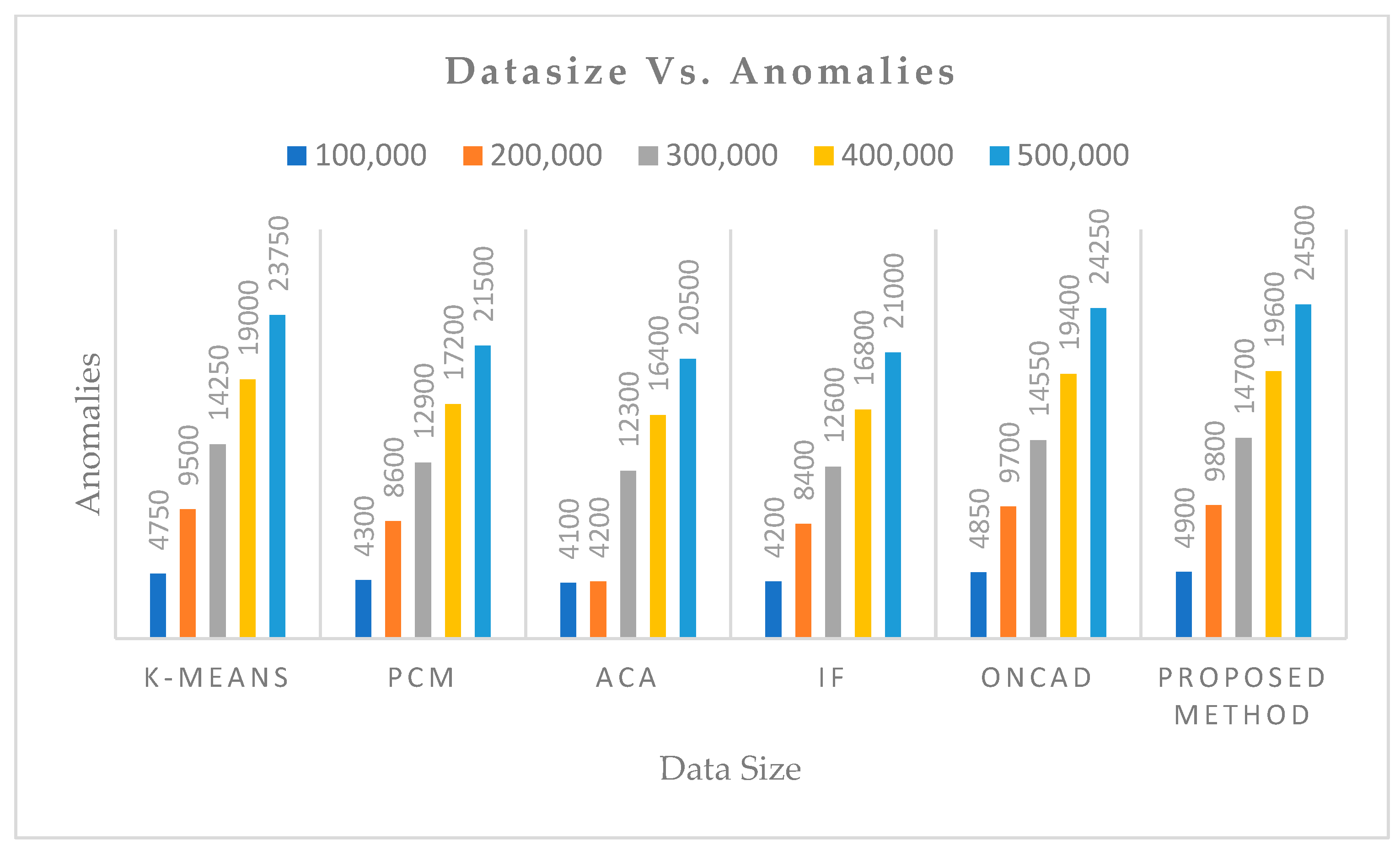
Thirdly, the temporal attributes are treated like any other attributes by aforesaid algorithms. However, the proposed algorithm treats temporal attributes (time-stamps) separately and produces the time-dependent clusters. Thus, each clusters will have a fuzzy life-time, and a data instance not falling within the lifetime or falling with a very low membership value or belonging to sparse cluster can be treated as an anomaly. That is why the proposed algorithm can extract more anomalies than others.

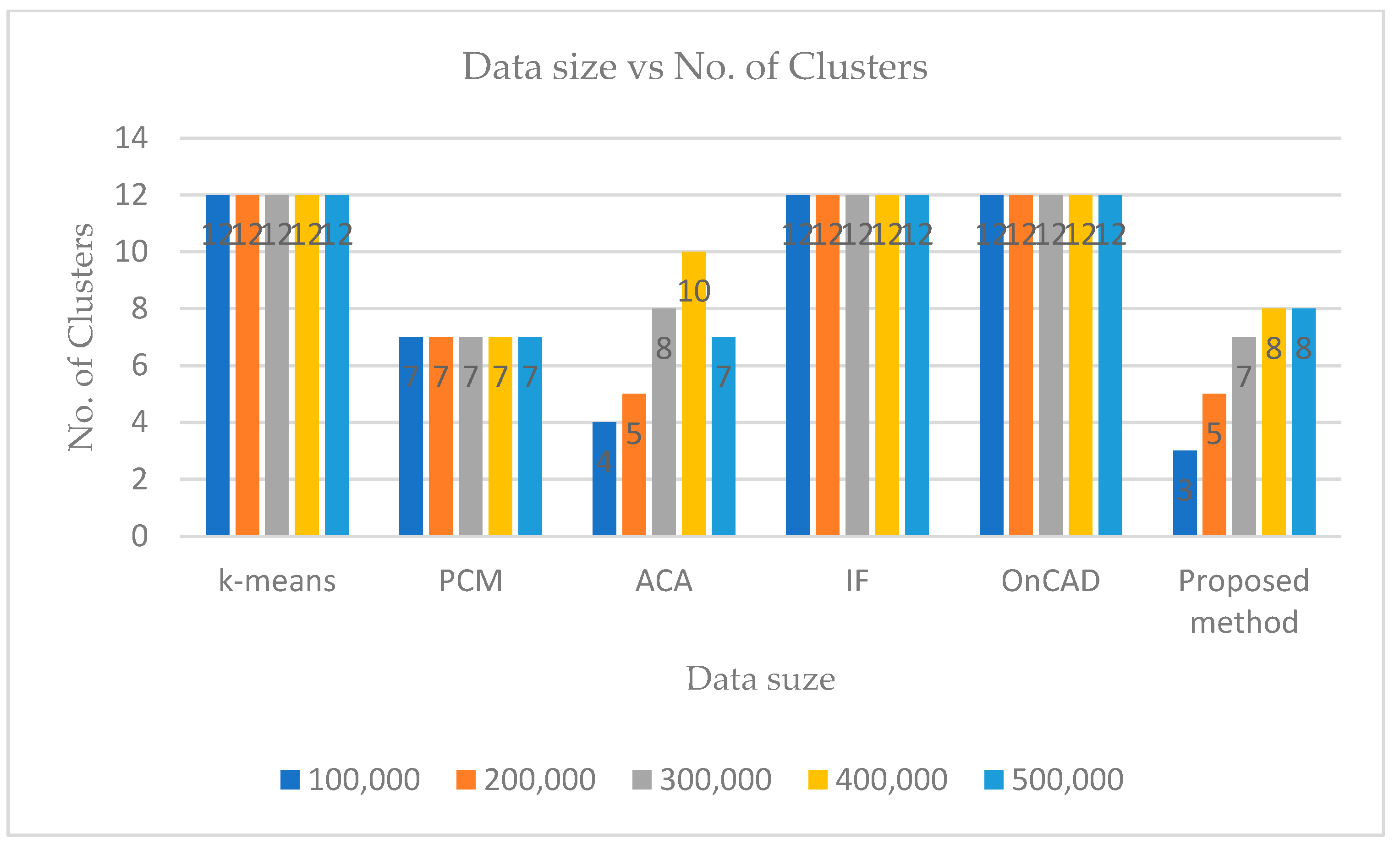
Finally, k-means and IF models give a specified number of clusters depending on the value of k chosen initially, which is not realistic in case of real-time clustering. If the time attribute is ignored or treated like any other attributes, PCM [14] gives better results, ACA does not give a reasonable solution as its output depends on order and number of inputs. OnCAD [31], needs a couple of input parameters to be specified. The proposed algorithm outperforms the aforesaid algorithms in the sense that it can handle higher dimensional data with numeric, categorical and temporal attributes better than others. 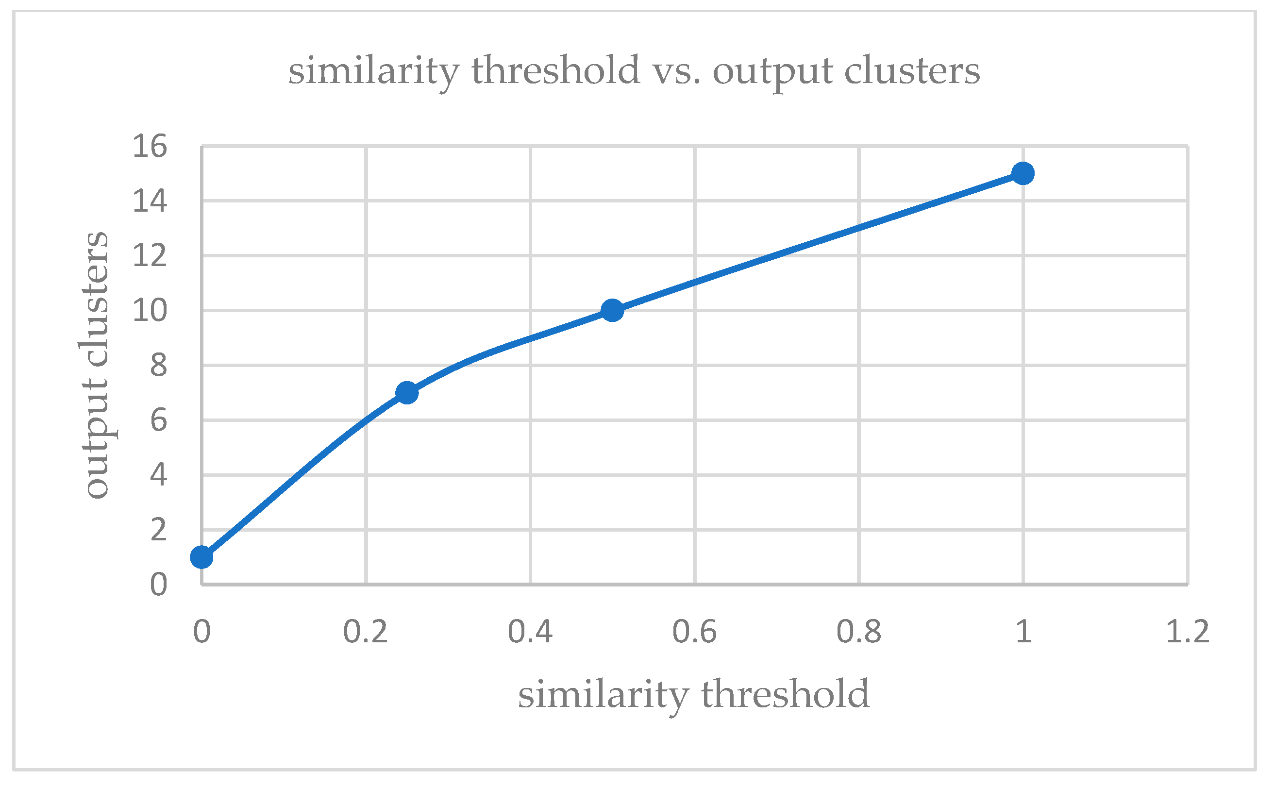Although the number of clusters k has to be specified in the partitioning phase, during phase two, the merge function minimizes the number of clusters. So, even if we start with a different number of input clusters, we arrive at quite a smaller number of stable clusters. For this experiment, the value of k is taken as 12 for KDDCup’99 [44] and 15 for Kitsune [45]. The similarity threshold has to be adjusted accordingly and in this case the values are taken as 0, 0.25, 0.5, 0.75. The obtained results corroborate our claim. Furthermore, the algorithm is scalable with respect to the data sizes. The algorithm’s time complexity is expressed graphically in Figure 8.

7. Conclusions, Limitations and Lines for Future Works

7.1. Conclusions

In this article, a clustering-based anomaly detection algorithm is proposed for real-time data with numeric and categorical attributes. The algorithm follows two-stage approach. Firstly, it follows k-means algorithmic approach and then an agglomerative hierarchical approach. The algorithm also takes into account the time-stamp associated with each data instance (the time of generation or occurrence of data). At the end of phase one, a set of k-clusters along with their lifetimes is found, where each cluster will have a lifetime. In the phase two, the similar clusters are merged depending on the non-empty intersections of their lifetimes. The algorithm stops when no further merger is possible. The proposed algorithm has the following features.

• It supplies a set of clusters, where each cluster will have an associated fuzzy time interval describing its period or lifetime.
• One of the most challenging issues in k-means algorithm is the selection of k. The proposed algorithm has overcome this problem by producing the same number of stable clusters, as the number of clusters reduces due to merging of clusters.
• Obviously, the number of output clusters is less than or equal to that at the beginning.
• The data instance or group of data instances, which does not belong to any of the cluster or belongs to sparse clusters or falling in the lifetime with very low membership values will be treated as anomalies.
• An experimental study with a synthetic dataset and a real world dataset is conducted and comparative analysis is carried out against a couple of clustering-based anomaly detection algorithms namely k-means [5], PCM (Partitioning clustering with merging) [14], ACA (agglomerative clustering algorithm) [39], IF (IsolationForest) [39], and OnCAD [31]. It has been found that our algorithm outperforms others in terms of accuracy, specificity, sensitivity, number of anomalies found, number of clusters generated, execution time and the stability of the output clusters.
• The algorithm is found to be run in cubic time.

7.2. Limitations and Lines for Future Works

Although our algorithm performs well in many cases, it still has some limitations. First of all, it has a limitation in finding anomaly from high-dimensional data with continuous attributes. Secondly, as it is based on k-means algorithm, it faces issues such as the centroid can be dragged by anomalies or anomalies may have their own clusters instead of being ignored. Finally, though it works nicely on time-stamp data, it lacks efficacy in dealing with temporal interval data.

Future works may proceed in the following directions:

• An efficient algorithm can be designed to find real-time anomalies in high-dimensional, heterogeneous data with continuous attributes.
• An efficient algorithm can be designed to find anomaly from temporal interval dataset.
• An approach other than partitioning and hierarchical viz. density based approach can be employed for the real-time anomaly detection.