Application of Discrete-Event Simulation for Truck Fleet Estimation at an Open-Pit Copper Mine in Peru

Abstract

With production expansions, studies related to estimating the number of pieces of hauling equipment to be employed in open-pit mines have to be carried out. One of the main challenges comes from the methodology selected since numerous tools are available, including commercial solutions. However, given that some methodologies were complex or required an advanced understanding of programming languages and that, in the case study, the mining company was applying a deterministic approach, a stochastic methodology that involves a discrete-event simulation (DES) was proposed. Such an approach aimed to develop a calibration model whose inputs incorporated random variables, such as fixed times and tonnages loaded to hauling equipment. This model supported the replication of the yearly production plan for an open-pit copper mine in Peru located at 4500 masl that is expanding its operations in 2023 from 100,000 tons per day to 140,000. The results obtained from the stochastic methodology were compared with the deterministic approach, which showed that the stochastic model required additional trucks and that longer cycle times were generated from such an approach. Such outputs are now supporting engineers in anticipating future problems in the mine due to the generation of longer queues.

1. Introduction

The loading and hauling process in a mining operation is one of the most important stages, as it represents around 50% to 60% of the total operating cost in an open-pit mine [1,2]. On the other hand, due to the variability in the nature of the variables that make up a shovel-truck system, the application of DES is feasible because it satisfactorily allows the recreation and estimation of system performance through time by means of the development of a simulation model [3,4]. Furthermore, there is a wide range in the application areas of the simulation because the consulted works addressed problems, such as minimization of maintenance cost and maximization of shovel availabilities, estimation of the haul truck fleet productivity, mining cost reduction, modeling and optimization of fuel consumption, and the optimization of the truck fleet size in an open-pit mine [5,6,7,8,9]. Nonetheless, regarding the truck fleet size estimation in open-pit mines, numerous studies employed complex methodologies, though innovative and effective, that involved an advanced understanding of programming languages, the development of neural network algorithms, or deterministic approaches [10,11,12,13,14,15,16,17,18,19,20,21]. For example, Tan & Takakuwa [19] developed an algorithm with VBA that included allocation planning—which found the maximum mining capacity and optimal truck fleet size—and dynamic allocation to find the best allocation scheduler. Ghaziani et al. [13] compared a flexible dispatching system to a Firefly Metaheuristic Algorithm using ARENA and MATLAB; the latter method increased production and reduced costs in an Iranian mine. Moradi Afrapoli et al. [10] developed a multiple-objective model with IBM CPLEX, ARENA, and MS Excel, maintaining the number of shovels during the simulation for one year, and the results showed a decrease in the required fleet size by 16% compared to a deterministic fleet size.

Moreover, commercial software packages addressing this problem are available in the market, including HaulSim, Talpac, and Haulage [22,23,24]. Some relevant features of these packages are that Talpac only works with a single loading unit at the time, Haulage can connect the cuts obtained from a mine plan through haul road profiles, and HaulSim allows the users to model bunching [3]. Because these solutions were designed exclusively for shovel-truck systems, they are closed-source simulation software.

Nowadays, given the presence of tools that enable the modeling of any process through the development of DES for free, such as Arena Software [25], and the extended literature covering this topic, the present work attempts to develop a non-dispatch methodology easy to understand for any user, new or experienced, in which having advanced programming language skills is not mandatory, but that allows the quick identification of possible errors during the simulation of truck-shovel systems. In addition, such an approach can be applied to other industries, such as manufacturing, shipping, and transport. In this work, the deterministic methodology employed in the case study was compared with the stochastic approach applied to a mine located at 4500 masl where scarce works have been developed. It was demonstrated that the former approach replicated the variability of the operating conditions, such as the fixed times and loaded tonnages by hauling equipment in an expanding open-pit copper mine located in Peru.

Thus, to solve the truck fleet estimation problem, probability distribution functions (PDF) and deviations from the random variables were collected as input, and from these distributions, the stochastic simulation developed different scenarios. Additionally, the Dijkstra algorithm was employed to solve the shortest path problem between origins and destinations [26]. On the other hand, the time required by loaded or unloaded trucks to travel was calculated with the different velocities by gradient. However, the present study differs from other works that aimed to optimize the haul truck fleet size by incorporating programming languages [27,28]. In this work, optimization was not the main goal. Instead, a non-dispatch solution was developed in which a specific number of trucks was assigned to certain loading equipment, and that number was varied until the planned production was reached for a certain simulation period. As a consequence, it was not necessary to calculate other factors, such as the match factor, which is helpful when seeking truck fleet productivity optimization.

This work first developed a calibrated model that was effective at replicating a yearly plan and demonstrated that stochastic models differed from deterministic approaches in the number of trucks required each month and other indicators, such as the number of hours worked by truck fleet, truck productivity, and the overall cycle time. The application of that methodology was tested in a Peruvian mining operation that produces copper concentrates and is going to expand its processing operations in 2023 from 100,000 tons to an estimated 140,000 tons per day during that year. Moreover, the company estimated its truck fleet size employing the traditional deterministic approach. It should be noted that another challenge came from the fact that research on the Peruvian mining industry is scarce, so this work also attempted to break with that history.

2. Methodology

This study aimed to calculate the necessary truck fleet size to fulfill the annual copper production of a mine using a discrete-event simulation methodology. This methodology was later compared with the deterministic approach to measure the impact on the truck fleet size between them. First, to achieve this goal, a 1-day operation model had to be calibrated because the main purpose of this was to recreate the existing operative conditions in the mine following step 2.1. After this process, the yearly plan was carried out, as shown in step 2.2.

2.1. Development of the Calibration Model

The methodology proposed by numerous authors recommends following the next steps [29,30,31].

Step 1. Gathering existing information and generation of probabilistic distribution functions.

Enough information related to the variables that intervene in the loading and hauling processes had to be gathered. Those variables included the tonnages loaded by existing equipment in the mine, fixed times of the cycle time, topographies, haul roads, and operating delays in the operation. Part of the previous information was obtained from a report generated by the CAT MineStar System. With the gathered information loaded in text (txt) format, the probabilistic distribution functions (PDF), density functions of the fixed times, and loaded tonnages were generated through Arena Input Analyzer, which helped to obtain distributions that fit the sample data. Anani & Awuah-Offei [29] and Owusu-Tweneboah et al. [4] described the analysis and modeling of the collected information in detail. The distributions were evaluated based on the Chi-square and Kolmogorov-Smirnov tests (KS) since Arena works with those tests to measure the goodness of the fit [2,10]. Regarding the variable times, mean values were chosen and obtained from the truck velocities according to the road grade and from the traveled distances. The traveled distances were calculated with the Dijkstra algorithm, whose objective is to obtain the shortest distance between two points.

Step 2. Creation and calibration of the model.

With the distribution functions of the fixed times and tonnages and the mean values of the variable times, processes and entities were created in the calibration model in Arena software. Furthermore, the target tonnages for the daily model were introduced as inputs. The steps taken to create the calibration model are presented in the following flowchart (Figure 1). In the loading and hauling process, trucks arrive at the loading areas where a shovel or FEL is rehandling either ore, stock, or waste material. These trucks are configured in Arena Software as entities, and they are assigned in groups to a fixed piece of loading equipment. Furthermore, each of the processes shown in Figure 1 is created in Arena following the order mentioned in the flowchart. At the beginning of the haul cycle, trucks might be queuing at the loading front or spotting if no other truck is present. Once the truck has spotted, the shovel or FEL might be ready to release the material onto the truck bed, which will depend on the available material. Depending on the loaded material, trucks might travel to the crusher, stockpile, or waste dump. After the loaded trucks arrive at their destination, they might queue or spot to finally release their material. Later, the haul cycle comes to an end, with the empty truck returning to the fixed loading front. At the end of the cycle, a delay time is added, which replicates operating stoppages happening in the mine. Arena Software allows the user to save the results from each process in a txt format, which is later processed through an Excel spreadsheet.

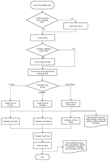
Figure 1. Calibration model flowchart.

Moreover, the calibration model did not consider truck stoppages for corrective maintenance or preventive maintenance; consequently, the entire truck fleet was always available. Other activities that did not factor into the calibration model were no operators available, limitations in the crushing rates, and lack of trucks. Finally, loading equipment applied the FIFO rule— first in, first out—which meant that the first truck arriving at the loading zone was given priority.

Step 3. Validation of results.

After the creation of the calibration model in Arena, the model was run, and the results obtained from it were compared with the real values from the Operations Team. The evaluated parameters were loaded tonnages by loading equipment, and total production. Based on the research conducted by Anani & Awuah-Offei [29], the number of replications for the calibration model was selected based on the half-width indicator in such a way that the difference between this indicator for each of the selected parameters and its mean values was less than 1%.

2.2. Yearly Plan Development

After the development and verification of the calibration model, deterministic and stochastic models were carried out for the 2023 yearly plan.

Step 1. Creation of the yearly model.

After verification of results produced by the calibration model in Arena, each of the 12 months from the 2023 yearly plan was modeled under the deterministic and stochastic approach. On the one hand, the probability distribution functions from the calibration model were maintained for the stochastic models, whereas mean values were utilized for the deterministic approach. On the other hand, target tonnages were modified according to the requirements of the yearly plan for each of the months to be simulated. Furthermore, variable and fixed times were calculated based on the new haul roads. It is worth noting that an additional front-end loader (FEL) was introduced around April of the next year, so a new cycle had to be modeled in Arena. Finally, the number of hours to simulate for each month was based on the planification of the yearly plan.

Step 2. Analysis of results.

After the creation and running of stochastic and deterministic models, the results produced were transformed into five indicators in order to explain the behavior of those developed models.

Truck productivity: Indicator measured in tons per hour and obtained as follows:

$$\mathrm{Productivity} (\mathrm{t}/\mathrm{h})=\frac{\mathrm{Tonnages} \mathrm{moved} \left(\mathrm{t}\right)}{(\mathrm{Total} \mathrm{Cycle} \mathrm{Time} (\min ) /60)}$$

(1)

Number of hours worked by truck fleet: Indicator calculated through the following expression.

$$\mathrm{Worked} \mathrm{hours}=\sum \frac{\mathrm{Tonnages} \mathrm{moved}}{\mathrm{Productivity}}$$

(2)

Overall cycle time: Calculated through the following expression.

$$\mathrm{Overall} \mathrm{Cycle} \mathrm{Time}=\frac{\sum \mathrm{Tonnages} \mathrm{moved}\times \mathrm{Total} \mathrm{Cycle} \mathrm{Time}}{\sum \mathrm{Tonnages} \mathrm{moved}}$$

(3)

Overall haul distance: Indicator measured in kilometers and obtained with the following formula.

$$\mathrm{Overall} \mathrm{Haul} \mathrm{Distance}=\frac{\sum \mathrm{Tonnages} \mathrm{moved}\times \mathrm{Traveled} \mathrm{Distance}}{\sum \mathrm{Tonnages} \mathrm{moved}}$$

(4)

Number of trucks: Obtained as the number of available trucks in the Arena model and divided by the mechanical availability planned in the month, and calculated as follows:

$$\mathrm{Required} \mathrm{Trucks}=\frac{\mathrm{Available} \mathrm{Trucks}}{\mathrm{Mechanical} \mathrm{Availability} (\%)}$$

(5)

3. Case Study

The study area covered an open-pit mine in Peru (Figure 2) that produces copper concentrates and is developing the expansion of its operations from 100,000 to 14,000 tons per day. The equipment present at the mine is made up of 29 CAT 797F haul trucks, 3 CAT 7495 rope shovels, and 2 LT-2350 FEL. Moreover, all the moved material goes to five destinations, including two waste dumps, a crusher, and three stockpiles.

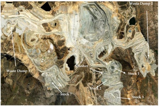
Figure 2. Layout of the Operations Area.

3.1. Calculations

First, the model was calibrated, and the above-mentioned steps were carried out in order to develop stochastic and deterministic models.

3.1.1. Development of the Calibration Model

Step 1. Gathering of existing information and generation of probabilistic distribution functions.

From a MineStar report, all the data were reviewed to later generate the probabilistic distribution functions and density functions of the fixed times and loaded tonnages through Arena Input Analyzer. Those results are presented in Tables 2 and 3. The functions employed by Arena Software were the normal distribution (NORM) and the beta distribution (BETA). It should be noted that Arena Input Analyzer recommends employing the function with the lowest square error after performing two goodness-of-fit tests. Those functions included Normal, Weibull, Beta, Triangular, Erlang, Gamma, Lognormal, Uniform, and Exponential. Furthermore, the information gathered from the MineStar report includes the results obtained in the operation, so it also involves the operator factor as their work affects the operating times and payloads. In addition, the attitude factor is implicit in the velocities employed for this work.

A demonstration of the Arena Input Analyzer to estimate the best distribution that fits the material loaded from the shovel 1 sample is shown next in Table 1. With 267 samples, the errors obtained from all the distributions available are as follows:

Table 1. Shovel 1 payload square errors for the functions tested with Arena Input Analyzer.

Function	Square Error
Normal	0.00211
Weibull	0.00301
Beta	0.00355
Triangular	0.00414
Erlang	0.00924
Gamma	0.00946
Lognormal	0.0192
Uniform	0.0311
Exponential	0.0582

Furthermore, Table 2 sums up the payload distribution, number of samples and errors obtained from the Kolmogorov-Smirnov and Chi-Square tests from all the loading equipment, whereas Table 3 shows the information related to the fixed times for trucks.

Table 2. PDF of the loaded tonnages for rope shovels and FEL.

Loading Equipment	Distribution	Expression	Sample Size	p-Value KS	Error
Shovel 1	Normal	NORM(375, 18.9)	267 samples	>0.15	0.002106
Shovel 2	Normal	NORM(370, 16.1)	240 samples	>0.15	0.006607
Shovel 3	Normal	NORM(376, 15.7)	256 samples	>0.15	0.003483
Front End Loader 3	Beta	321 + 96 × BETA(1.82, 2.96)	96 samples	>0.15	0.007573
Front End Loader 1	Normal	NORM(357, 13.9)	75 samples	>0.15	0.007145

Table 2. PDF of the loaded tonnages for rope shovels and FEL.

Loading Equipment	Distribution	Expression	Sample Size	p-Value KS	Error
Shovel 1	Normal	NORM(375, 18.9)	267 samples	>0.15	0.002106
Shovel 2	Normal	NORM(370, 16.1)	240 samples	>0.15	0.006607
Shovel 3	Normal	NORM(376, 15.7)	256 samples	>0.15	0.003483
Front End Loader 3	Beta	321 + 96 × BETA(1.82, 2.96)	96 samples	>0.15	0.007573
Front End Loader 1	Normal	NORM(357, 13.9)	75 samples	>0.15	0.007145

Table 3. PDF of the fixed times for trucks.

Type Time	Distribution	Expression	Sample Size	p-Value KS	Error
Truck arrival	Normal	NORM(4.18, 1.03)	128 samples	>0.15	0.016269
Spotting at Shovel 1	Beta	0.73 + 0.84 × BETA(1.37, 1.46)	267 samples	>0.15	0.003612
Waiting for load at Shovel 1	Beta	0.01 + 0.87 × BETA(8.67, 12.5)	267 samples	>0.15	0.003061
Loading time at Shovel 1	Beta	1.76 + 1.24 × BETA(3.3, 3.31)	267 samples	>0.15	0.002285
Spotting at Shovel 2	Beta	0.73 + 0.83 × BETA(1.21, 1.68)	240 samples	>0.15	0.006755
Waiting for load at Shovel 2	Beta	0.01 + 0.87 × BETA(6.96, 7.49)	240 samples	>0.15	0.00519
Loading time at Shovel 2	Normal	NORM(2.32, 0.164)	240 samples	>0.15	0.004032
Spotting at Shovel 3	Normal	NORM(1.09, 0.136)	256 samples	>0.15	0.017094
Waiting for load at Shovel 3	Beta	0.03 + 0.85 × BETA(6.54, 10.1)	256 samples	>0.15	0.002007
Loading time at Shovel 3	Beta	1.78 + 1.35 × BETA(5.66, 9.83)	256 samples	0.0518	0.009006
Spotting at FEL 3	Beta	0.75 + 0.8 × BETA(4.75, 6.34)	96 samples	>0.15	0.011225
Waiting for load at FEL 3	Beta	0.07 + 1.07 × BETA(0.917, 1.4)	96 samples	>0.15	0.033927
Loading time at FEL 3	Beta	4.52 + 2.15 × BETA(7.7, 7.97)	96 samples	>0.15	0.003864
Spotting at FEL 1	Normal	NORM(1.08, 0.0938)	75 samples	>0.15	0.000836
Waiting for load at FEL 1	Beta	0.15 + 0.69 × BETA(3.27, 3.12)	75 samples	>0.15	0.008227
Loading time at FEL 1	Normal	NORM(5.62, 0.248)	75 samples	>0.15	0.005183
Spotting at Crusher	Normal	NORM(1.55, 0.0621)	150 samples	>0.15	0.002465
Unloading time at Crusher	Normal	NORM(0.882, 0.0271)	150 samples	>0.15	0.003761
Spotting at Stockpile	Beta	0.88 + 0.17 × BETA(5.42, 5.89)	160 samples	>0.15	0.002049
Unloading time at Stockpile	Normal	NORM(0.912, 0.021)	160 samples	>0.15	0.005051
Spotting at Waste Dump	Normal	NORM(0.945, 0.0264)	148 samples	>0.15	0.002304
Unloading time at Waste Dump	Normal	NORM(0.911, 0.0266)	148 samples	>0.15	0.00675

Table 3. PDF of the fixed times for trucks.

Type Time	Distribution	Expression	Sample Size	p-Value KS	Error
Truck arrival	Normal	NORM(4.18, 1.03)	128 samples	>0.15	0.016269
Spotting at Shovel 1	Beta	0.73 + 0.84 × BETA(1.37, 1.46)	267 samples	>0.15	0.003612
Waiting for load at Shovel 1	Beta	0.01 + 0.87 × BETA(8.67, 12.5)	267 samples	>0.15	0.003061
Loading time at Shovel 1	Beta	1.76 + 1.24 × BETA(3.3, 3.31)	267 samples	>0.15	0.002285
Spotting at Shovel 2	Beta	0.73 + 0.83 × BETA(1.21, 1.68)	240 samples	>0.15	0.006755
Waiting for load at Shovel 2	Beta	0.01 + 0.87 × BETA(6.96, 7.49)	240 samples	>0.15	0.00519
Loading time at Shovel 2	Normal	NORM(2.32, 0.164)	240 samples	>0.15	0.004032
Spotting at Shovel 3	Normal	NORM(1.09, 0.136)	256 samples	>0.15	0.017094
Waiting for load at Shovel 3	Beta	0.03 + 0.85 × BETA(6.54, 10.1)	256 samples	>0.15	0.002007
Loading time at Shovel 3	Beta	1.78 + 1.35 × BETA(5.66, 9.83)	256 samples	0.0518	0.009006
Spotting at FEL 3	Beta	0.75 + 0.8 × BETA(4.75, 6.34)	96 samples	>0.15	0.011225
Waiting for load at FEL 3	Beta	0.07 + 1.07 × BETA(0.917, 1.4)	96 samples	>0.15	0.033927
Loading time at FEL 3	Beta	4.52 + 2.15 × BETA(7.7, 7.97)	96 samples	>0.15	0.003864
Spotting at FEL 1	Normal	NORM(1.08, 0.0938)	75 samples	>0.15	0.000836
Waiting for load at FEL 1	Beta	0.15 + 0.69 × BETA(3.27, 3.12)	75 samples	>0.15	0.008227
Loading time at FEL 1	Normal	NORM(5.62, 0.248)	75 samples	>0.15	0.005183
Spotting at Crusher	Normal	NORM(1.55, 0.0621)	150 samples	>0.15	0.002465
Unloading time at Crusher	Normal	NORM(0.882, 0.0271)	150 samples	>0.15	0.003761
Spotting at Stockpile	Beta	0.88 + 0.17 × BETA(5.42, 5.89)	160 samples	>0.15	0.002049
Unloading time at Stockpile	Normal	NORM(0.912, 0.021)	160 samples	>0.15	0.005051
Spotting at Waste Dump	Normal	NORM(0.945, 0.0264)	148 samples	>0.15	0.002304
Unloading time at Waste Dump	Normal	NORM(0.911, 0.0266)	148 samples	>0.15	0.00675

Next, the velocities employed along with the Dijkstra algorithms are presented in Table 4.

Table 4. Velocities reached by trucks according to road grade.

Grade (%)	Velocity When Loaded (km/h)	Velocity When Empty (km/h)	Grade (%)	Velocity When Loaded (km/h)	Velocity When Empty (km/h)
−12	14.3	30.8	12	10.5	12.7
−11	14.3	30.8	11	10.5	12.7
−10	14.3	30.8	10	10.5	12.7
−9	16.9	32.3	9	12.0	15.2
−8	19.6	33.8	8	13.4	17.6
−7	22.2	35.3	7	14.9	20.0
−6	24.9	36.8	6	16.3	22.4
−5	27.5	38.3	5	17.8	24.8
−4	29.0	39.8	4	21.2	29.0
−3	30.4	41.4	3	24.6	33.3
−2	31.9	42.9	2	28.0	37.5
−1	33.3	44.4	1	31.4	41.7
0	34.8	45

Step 2. Creation and calibration of the model.

On the day to be simulated, there were five pieces of loading equipment, including three rope shovels and two FELs. Moreover, trucks operated under a mechanical availability of 83.43%, and at the end of the day, approximately 330,000 tons were moved. Table 5 shows the moved material and the material and destinations reached that day.

Table 5. Results to replicate by the simulation.

Equipment/Destination	Crusher	Stock 1	Stock 2	Stock 3	Waste Dump 2
Shovel 1	58,762		39,558	10,400
Shovel 2	42,276	36,962		13,500	766
Shovel 3		13,443		38,987	43,776
FEL 3					17,257
FEL 1					17,066
Total Tonnage	101,038	50,405	39,558	62,887	78,865

From the gathered information, it was determined that trucks worked 10-h shifts a day with 2 h corresponding to operating delays as a result of shift change, equipment check, blasting, or lunch breaks.

Step 3. Validation of results

There were 100 simulations considered fulfilling a difference of less than 1% between the half-width indicators of the loaded tonnages using loading equipment and total production and those indicators’ mean values. Thus, the following results (Table 6) from the calibration model were obtained:

Table 6. Validation of the calibration model.

Parameters	Real	Simulation		Error
		Mean	Half-Width
Total Production	332,752.3	334,780.1	107.1	0.61%
Moved Tons Shovel 1	108,720.0	109,236.0	56.8	0.47%
Moved Tons Shovel 2	93,503.3	94,376.5	52.3	0.93%
Moved Tons Shovel 3	96,206.0	96,474.6	86.5	0.28%
Moved Tons FEL 3	17,257.0	17,457.7	23.3	1.15%
Moved Tons FEL 1	17,066.0	17,235.3	24.0	0.98%

From Table 6, the maximum prediction error for all the parameters was 1.15%. Having small error values is critical, considering that the more time is simulated, the more the deviation from the simulated output values.

After 100 simulations for a 20-h day, all the information from the Arena model was processed, and the following results were obtained (Figure 3).

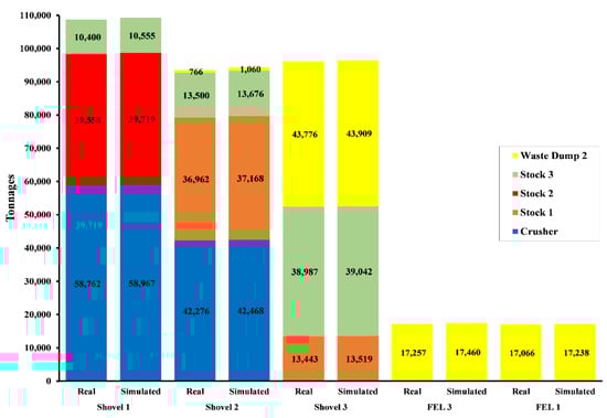
Figure 3. Real tonnages versus simulated results.

In Figure 3, it can be observed that real tonnages moved during the chosen day were almost similar to the results obtained from the simulation. This difference could be reduced even more if the bucket payload was added, as this restriction would limit the total tonnage to load, and the result would be closer to the real tonnage.

Regarding the number of trucks employed by the simulation for each piece of loading equipment, the simulation required 24 trucks in total during that day, as shown in Table 7.

Table 7. Truck distribution for each piece of loading equipment.

Equipment	Number of Trucks
Shovel 1	6
Shovel 2	7
Shovel 3	7
FEL 3	2
FEL 1	2

Considering that the mechanical availability that day was 83.43%, and the number of trucks required by the model was 24, then by applying Equation (5), the number of trucks in the truck fleet was 29. This figure was equal to the number of trucks used in the operation. On the other hand, the behavior of the overall cycle time reflected the times at the mine operation. These values are shown in Figure 4.

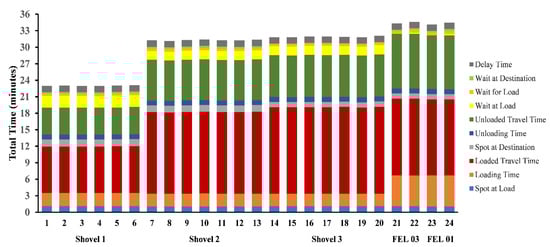
Figure 4. Truck cycle time for each loading equipment.

These truck cycle times were reviewed for each destination to check whether they reflected the real cycle times at the mine or not. Otherwise, the velocities, road grades, or PDF would have been reviewed. Figure 5, Figure 6, Figure 7 and Figure 8 show the behavior of these cycle times.

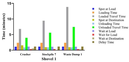
Figure 5. Total cycle time for trucks assigned to shovel 1.

Figure 6. Total cycle time for trucks assigned to shovel 2.

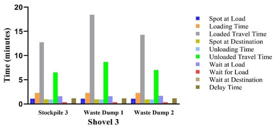
Figure 7. Total cycle time for trucks assigned to shovel 3.

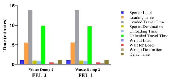
Figure 8. Total cycle time for trucks assigned to FELs.

After having reviewed the results generated by the simulation, the yearly plan was developed.

3.1.2. Yearly Plan Development

Having developed the calibration model, a model was created for each of the months within the yearly plan, applying first a stochastic methodology. Among the information given with the yearly plan, the different destinations could be found where the tonnages would end up, the number of days for each month, and the planned mechanical availability for the truck fleet. Additionally, due to a change in the material handling, stockpiles 1 and 2 stopped receiving trucks, and stockpiles 3 and 7 were deposited with ore as new designs allowed the expansion of those piles, thus increasing their total capacity.

Step 1. Creation of the yearly model

The month-to-month planned tonnages varied, as shown in Figure 9. Furthermore, the overall daily tons moved month-to-month was increased from 325,000 tons in January to 386,000 tons in December, maintaining this value consistently since July.

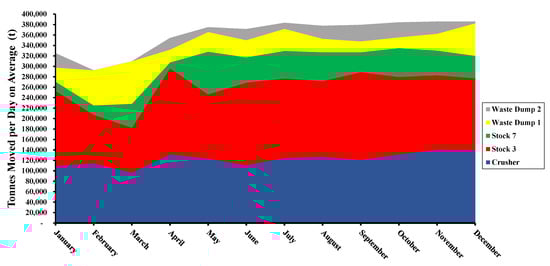
Figure 9. Tons moved per day on average during 2023.

It is worth noting that the number of days in the plan for each month was based on the Asiatic calendar, which is different from the Gregorian calendar, as the number of days per month is not regular, see Table 8.

Table 8. Number of days per month in the Asiatic calendar.

Month	Number of Days	Month	Number of Days
January	25	July	30
February	31	August	31
March	29	September	31
April	31	October	30
May	30	November	31
June	31	December	36

Moreover, the month-to-month mechanical availability for the truck fleet varied, as shown in Table 9.

Table 9. Fleet mechanical availability planned for the year.

Month	Mechanical Availability (%)	Month	Mechanical Availability (%)
January	80.55	July	81.82
February	80.35	August	82.06
March	82.08	September	81.94
April	81.92	October	81.84
May	81.9	November	81.82
June	81.96	December	82.99

Step 2. Analysis of results

In the simulation for each of the models, there were variations in the truck fleet numbers in certain months. However, these changes did not vary that much at first sight, so several indicators were analyzed to explain these variations between the stochastic and deterministic models.

-

Number of hours worked by truck fleet: In Figure 10, the number of hours required between these two models is shown.

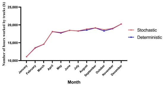Figure 10. Number of hours worked by truck fleet in the deterministic and stochastic models.

-

Truck productivity: By increasing the overall cycle time, the truck productivity was then reduced. In Figure 11, the results obtained from these models are compared.

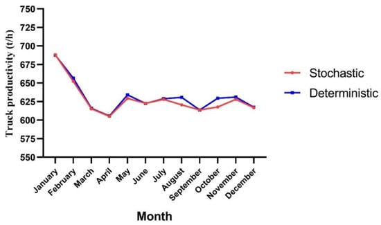Figure 11. Truck productivity in the stochastic and deterministic models.

-

Overall cycle time: The results obtained are shown in Figure 12.

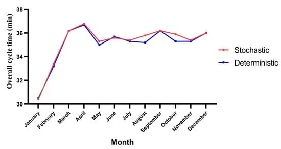Figure 12. Overall cycle time in the stochastic and deterministic models.

-

Overall haul distance: In Figure 13, the overall haul distance traveled by trucks over twelve months can be seen.

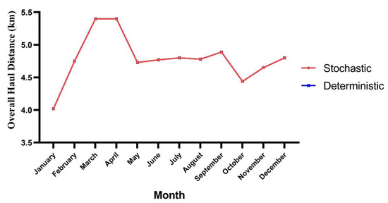Figure 13. Overall haul distance in the stochastic and deterministic models.

-

Number of trucks: Clearly, in Figure 14, the results produced by the models estimated an increase in the number of trucks starting from 30 up to 42 by the end of 2023.

Figure 14. Number of required trucks in the stochastic and deterministic models.

4. Results and Discussion

Regarding the results of the main indicators generated for the yearly plan in Figure 10, Figure 11, Figure 12, Figure 13 and Figure 14, the following explanations were given.

4.1. Number of Hours Worked by Truck Fleet

From Figure 10, it was found that there was a similar requirement between both models in the number of hours. However, more hours were demanded by the stochastic model, in general. Further, analyzing the hours month to month, in Figure 10, there was a greater number of hours required in December, as the number of days during that month was 36, and the overall cycle time increased compared with the 31 days from November. On the other hand, the most visible variations between both models occurred in August and October as the cycle times in the stochastic model for those months increased, given the longer queues at the loading equipment. More of these queue times are mentioned in Section 4.3. Finally, that increment subsequently affected the truck fleet productivity during those months for the stochastic model.

4.2. Truck Productivity

As mentioned in Equation (1), truck productivity will rely on the tonnages moved and the overall cycle time. From Figure 11, the fall in productivity between January and April occurred as a consequence of the increment in the overall cycle time by six minutes. Moreover, the tonnages moved in the months after April were maintained almost at a constant rate with minimal variation in the overall cycle time. Consequently, the truck productivity behaved similarly during those months.

4.3. Overall Cycle Time

Given the mine expansion in 2023, it was observed in Figure 12 that the overall cycle time increased from 30.4 min in January to 36 min in December. Another variation came from the months of August and October, which was the result of an increase of 30 s in the waiting time at the loading equipment and destinations assigned during those months. On the one hand, for the stochastic model in August, the queues generated at the loading equipment were 25 s longer compared with the deterministic model, and 10 additional seconds were added to the overall cycle time in that month for the stochastic model compared with the deterministic model. On the other hand, the queues at the loading fronts in October were 34 s longer for the stochastic model, and 6 additional seconds were added to the cycle time at the destination points for the stochastic model during that period. In both cases, the increments were the result of the bunching of trucks due to shorter distances to travel and the fall in planned tonnages.

4.4. Overall Haul Distance

As mining engineers set a plan to reach the desired copper production established by the company in 2023, the exploitation of benches in lower levels made haul road distances increase from 4 km in January up to 4.8 km in December and reached a peak of 5.4 km in March and April due to the longer travel distances to dump waste material. Moreover, trucks from both models traveled the same distance, as shown in Figure 13.

4.5. Number of Trucks

It was noted that the results produced by the models, shown in Figure 14, estimated an increase in the number of trucks starting from 30 up to 42 by the end of 2023. Nonetheless, this month-to-month increment varied according to the selected model. This difference came from the overall cycle time, overall haul distance, and tonnage to move. Moreover, the most noticeable difference between the models came from February, whereas in the rest of the months, the variation was one truck or none. Although the number of hours worked by the truck fleet and the overall cycle time from the deterministic and stochastic models were almost similar in February, when the mechanical availability was applied, the initial variation from those models increased from one up to two.

Then, the results are discussed as follows:

First, the results produced from the methodology showed that stochastic models differed from deterministic models in the longer queues at loading points, which were, in the end, translated as an increment in the number of required trucks for the yearly plan in almost every month. Additionally, the longer queues were generated as a consequence of the variability of the fixed times, and that effect had an impact on the other indicators reviewed, such as longer haul cycles and lower productivities and working hours. A great benefit produced from the proposed methodology is the simplicity in recreating the variability of the parameters present at the mining operation, which allowed the saving of time. Moreover, those parameters could be modified as many times as required.

On the other hand, the queues generated at the mining fronts have to be reduced as a next step. However, the present work did not intend to optimize the haul fleet size or to increase truck productivity, and there are numerous studies that have covered these fields with a strong mathematical framework. In the study developed by Moradi Afrapoli et al. [10], researchers worked with a multiple-objective model capable of meeting the production requirement in an open-pit iron mine, requiring 85% of the fleet size of a deterministic model. Furthermore, Ozdemir & Kumral [2] were able to increase the productivity of truck and shovel systems by employing the match factor along with the dispatching system while reducing the truck queues and shovel idle times.

5. Conclusions

This study determined that 13 additional haul trucks were required for the case study by developing either a stochastic or a deterministic approach. Nonetheless, the number of trucks required from a stochastic approach differed from the results produced by a deterministic model in certain months.

On the other hand, a DES methodology was developed in this work, which showed clear evidence of the impact produced by the variability of the parameters from the loading and hauling processes on the truck fleet size obtained from these models. That impact was reflected in each of the indicators studied in the present study, such as the number of hours worked by the truck fleet, truck productivity, and overall cycle times.

Finally, in order to continue improving the stochastic model, future work will focus on the reduction in the queue times and the increment of productivity by working with simulation optimization tools.

References

- Ahumada, G.I.; Herzog, O. Application of multiagent system and tabu search for truck dispatching in open-pit mines. In Proceedings of the ICAART 2021—Proceedings of the 13th International Conference on Agents and Artificial Intelligence, Vienna, Austria, 4–6 February 2021; Volume 1, pp. 160–172. [Google Scholar] [CrossRef]
- Ozdemir, B.; Kumral, M. Simulation-based optimization of truck-shovel material handling systems in multi-pit surface mines. Simul. Model. Pract. Theory 2019, 95, 36–48. [Google Scholar] [CrossRef]
- Baafi, E.Y.; Zeng, W. A discrete-event simulation for a truck-shovel system. In Proceedings of the 27th International Symposium on Mine Planning and Equipment Selection—MPES 2018; Springer International Publishing: Berlin/Heidelberg, Germany, 2019. [Google Scholar] [CrossRef]
- Owusu-Tweneboah, M.; Temeng, V.A.; Awuah-Offei, K. Agent-based optimization for truck dispatching in open-pit mines. In Proceedings of the 2019 SME Annual Conference and Expo and CMA 121st National Western Mining Conference, Denver, CO, USA, 24–27 February 2019; pp. 1–4. [Google Scholar]
- Gao, Y.; Ai, Y.; Tian, B.; Chen, L.; Wang, J.; Cao, D.; Wang, F.Y. Parallel end-to-end autonomous mining: An IoT-oriented approach. IEEE Internet Things J. 2020, 7, 1011–1023. [Google Scholar] [CrossRef]
- Golbasi, O.; Kina, E. Haul truck fuel consumption modeling under random operating conditions: A case study. Transp. Res. Part D Transp. Environ. 2022, 102, 103135. [Google Scholar] [CrossRef]
- Golbasi, O.; Turan, M.O. A discrete-event simulation algorithm for the optimization of multi-scenario maintenance policies. Comput. Ind. Eng. 2020, 145, 106514. [Google Scholar] [CrossRef]
- Moradi Afrapoli, A.; Tabesh, M.; Askari-Nasab, H. A stochastic hybrid simulation-optimization approach towards haul fleet sizing in surface mines. Min. Technol. Trans. Inst. Min. Metall. 2019, 128, 9–20. [Google Scholar] [CrossRef]
- Upadhyay, S.; Tabesh, M.; Badiozamani, M.; Askari-Nasab, H. A Simulation Model for Estimation of Mine Haulage Fleet Productivity; Springer: Cham, Switzerland, 2020. [Google Scholar]
- Moradi Afrapoli, A.; Tabesh, M.; Askari-Nasab, H. A multiple objective transportation problem approach to dynamic truck dispatching in surface mines. Eur. J. Oper. Res. 2019, 276, 331–342. [Google Scholar] [CrossRef]
- Bakhtavar, E.; Mahmoudi, H. Development of a scenario-based robust model for the optimal truck-shovel allocation in open-pit mining. Comput. Oper. Res. 2018, 115, 104539. [Google Scholar] [CrossRef]
- Baek, J.; Choi, Y. Deep neural network for predicting ore production by truck-haulage systems in open-pit mines. Appl. Sci. 2020, 10, 1657. [Google Scholar] [CrossRef]
- Ghaziani, H.H.; Monjezi, M.; Mousavi, A.; Dehghani, H.; Bakhtavar, E. Design of loading and transportation fleet in open-pit mines using simulation approach and metaheuristic algorithms. J. Min. Environ. 2021, 12, 1175–1186. [Google Scholar] [CrossRef]
- Both, C.; Dimitrakopoulos, R. Joint stochastic short-term production scheduling and fleet management optimization for mining complexes. Optim. Eng. 2020, 21, 1717–1743. [Google Scholar] [CrossRef]
- Lisboa, A.C.; De Souza, F.H.B.; Ribeiro, C.M.; Maia, C.A.; Saldanha, R.R.; Castro, F.L.B.; Vieira, D.A.G. On modelling and simulating open pit mine through stochastic timed petri nets. IEEE Access 2019, 7, 112821–112835. [Google Scholar] [CrossRef]
- Mohtasham, M.; Mirzaei-Nasirabad, H.; Alizadeh, B. Optimization of truck-shovel allocation in open-pit mines under uncertainty: A chance-constrained goal programming approach. Min. Technol. Trans. Inst. Min. Metall. 2021, 130, 81–100. [Google Scholar] [CrossRef]
- Upadhyay, S.P.; Tabesh, M.; Badiozamani, M.M.; Moradi Afrapoli, A.; Askari-Nasab, H. A simulation-based algorithm for solving surface mines’ equipment selection and sizing problem under uncertainty. CIM J. 2021, 12, 36–46. [Google Scholar] [CrossRef]
- Zhang, S.; Lu, C.; Jiang, S.; Shan, L.; Xiong, N.N. An unmanned intelligent transportation scheduling system for open-pit mine vehicles based on 5G and big data. IEEE Access 2020, 8, 135524–135539. [Google Scholar] [CrossRef]
- Tan, Y.; Takakuwa, S. A practical simulation approach for an effective truck dispatching system of open pit mines using VBA. In Proceedings of the Winter Simulation Conference, Washington, DC, USA, 11–14 December 2016; pp. 2394–2405. [Google Scholar]
- Cox, W.; French, T.; Reynolds, M.; While, L. A genetic algorithm for truck dispatching in mining. GCAI 2018, 50, 93–107. [Google Scholar] [CrossRef]
- Nobahar, P.; Pourrahimian, Y.; Mollaei Koshki, F. Optimum fleet selection using machine learning algorithms—Case study: Zenouz Kaolin mine. Mining 2022, 2, 528–541. [Google Scholar] [CrossRef]
- RPM Global HAULSIM. Available online: https://rpmglobal.com/product/haulsim (accessed on 1 November 2022).
- RPM Global TALPAC-3D. Available online: https://rpmglobal.com/product/talpac-3d (accessed on 1 November 2022).
- HEXAGON HxGN MinePlan OP Short-Term Planning. Available online: https://hexagon.com/products/hxgn-mineplan-open-pit-engineering-short-term (accessed on 1 November 2022).
- Rockwell Automation Arena Simulation Software. Available online: https://www.rockwellautomation.com/en-us/products/software/arena-simulation.html (accessed on 31 August 2022).
- Moradi Afrapoli, A.; Askari-Nasab, H. Mining fleet management systems: A review of models and algorithms. Int. J. Min. Reclam. Environ. 2017, 33, 42–60. [Google Scholar] [CrossRef]
- Guseva, E.; Efimova, I.; Varfolomeyeva, T. Simulation modeling of transport flows of copper deposit. In Proceedings of the 2019 International Science and Technology Conference “EastConf”, Vladivostok, Russia, 1–2 March 2019; pp. 1–4. [Google Scholar] [CrossRef]
- Mohtasham, M.; Mirzaei-Nasirabad, H.; Askari-Nasab, H.; Alizadeh, B. Truck fleet size selection in open-pit mines based on the match factor using a MINLP model. Min. Technol. Trans. Inst. Min. Metall. 2021, 130, 159–175. [Google Scholar] [CrossRef]
- Anani, A.; Awuah-Offei, K. Incorporating changing duty cycles in CM-shuttle car matching using discrete event simulation: A case study. Int. J. Min. Miner. Eng. 2017, 8, 96–112. [Google Scholar] [CrossRef]
- Dumakor-Dupey, N.K.; Temeng, V.A.; Bansah, K.J. Optimising shovel-truck fuel consumption using stochastic simulation. Ghana Min. J. 2017, 17, 39–49. [Google Scholar] [CrossRef]
- Medina, X.; Vásquez, J.; Noriega, R.; Moreno-Chavez, J. Loading-haulage system assessment using discrete event simulation. In Proceedings of the 17th LACCEI International Multi-Conference for Engineering, Education and Technology, Montego Bay, Jamaica, 24–26 July 2019. [Google Scholar] [CrossRef]
Disclaimer/Publisher’s Note: The statements, opinions and data contained in all publications are solely those of the individual author(s) and contributor(s) and not of MDPI and/or the editor(s). MDPI and/or the editor(s) disclaim responsibility for any injury to people or property resulting from any ideas, methods, instructions or products referred to in the content. |
© 2023 by the authors. Licensee MDPI, Basel, Switzerland. This article is an open access article distributed under the terms and conditions of the Creative Commons Attribution (CC BY) license (https://creativecommons.org/licenses/by/4.0/).