Featured Application
Computation of Relaxation Time Maps in Magnetic Resonance Imaging.
Abstract
Magnetic resonance imaging (MRI) is a valuable diagnostic tool that provides detailed information about the structure and function of tissues in the human body. In particular, measuring relaxation times, such as T1 and T2, can provide important insights into the composition and properties of different tissues. Accurate relaxation time mapping is therefore critical for clinical diagnosis and treatment planning, as it can help to identify and characterize pathological conditions, monitor disease progression, and guide interventions. However, the computation of relaxation time maps in MRI is a complex and challenging task that requires sophisticated mathematical algorithms. Thus, there is a need for robust and accurate algorithms that can reliably extract the desired information from MRI data. This article compares the performance of the Reduced Dimension Nonlinear Least Squares (RD-NLS) algorithm versus several widely used algorithms to compute relaxation times in MRI, such as Levenberg-Marquardt and Nelder-Mead. RD-NLS simplifies the search space for the optimum fit by leveraging the partial linear relationship between signal intensity and model parameters. The comparison was performed on several datasets and signal models, resulting in T1 and T2 maps. The algorithms were evaluated based on their fit error, with the RD-NLS algorithm showing a lower error than other fit-ting algorithms. The improvement was particularly notable in T1 maps, with less of a difference in T2 maps. Additionally, the average T1 values computed with different algorithms differed by up to 14 ms, indicating the importance of algorithm selection. These results suggest that the RD-NLS algorithm outperforms other commonly used algorithms for computing relaxation times in MRI.
1. Introduction
Magnetic Resonance Imaging (MRI) uses magnetic fields and radio waves to create detailed body images. The intensity of the signal in an MRI image is influenced by various factors, including relaxation times. These times are constants that indicate the magnetic properties of the tissue being imaged. Images that show the relaxation times for each pixel in the image are called relaxation time maps. Accurate relaxation time mapping in MRI is crucial for clinical diagnosis and treatment planning. T1 and T2 relaxation times are sensitive to tissue composition, microstructure, and other physiological properties. These maps have many uses in both research and clinical settings, such as determining the amount of Myocardial Extracellular Volume (ECV) in the heart [1], detecting edema in cases of acute myocardial infarction [2], identifying early tumor progression in the brain [3], differentiating between healthy and early degenerative cartilage [4], or providing helpful information to classify between normal and pathological brain aging [5]. Accurate relaxation time mapping is, therefore, critical for identifying and characterizing disease, monitoring its progression, and guiding interventions such as radiation therapy or surgical resection. Additionally, there is growing interest in using quantitative MRI for research in other areas, such as food products and processing [6]. Moreover, the choice of the algorithm used for relaxation time mapping can have a significant impact on the accuracy and precision of the resulting maps. To improve the accuracy of MRI data and reduce errors, it is important to continue developing new models and algorithms for processing MRI data, which will reduce variability and facilitate a more accurate diagnosis/classification [7].
Relaxation times that are routinely measured in MR are longitudinal or spin-lattice relaxation time (T1), transversal or spin-spin relaxation time (T2), and apparent transversal relaxation time (T2*) [8,9,10]. In what follows, this will be referred to as “relaxation time” (Trel). The type of pulse sequence and the technical parameters used during the acquisition determine how each time factor affects the final signal intensity. For a detailed description of MR signal formation, the reader is referred to the textbooks on this topic [11,12,13].
Creating relaxation time maps in MRI is a multi-step process because the MR signal is affected by various factors. A group of MR pulse sequences is used to generate the maps, with different techniques listed in Table 1. The basic concept behind most of these methods is to acquire a set of images with similar imaging parameters, except for one, such as repetition time (TR), echo time (TE), inversion time (TI), or saturation time (TS). This parameter is referred to as the “time parameter” (T). Once the images are acquired, a pixel-by-pixel curve fitting analysis is done according to a theoretical equation that describes the physical phenomena behind the process. This analysis produces the desired quantitative maps.

Table 1.
Some MRI signal models can be fitted using the algorithm described in this manuscript. The fit can be partially linearized in all cases, so only one parameter (relaxation time) needs to be varied to find the lowest error.
As it is clear from the formulas in Table 1, nonlinear regression is needed to fit the data to obtain relaxation times. A widely used method to obtain the optimum fit is to minimize the sum of the squares of the differences between predicted and measured signals. In this context, the predicted signal is the value predicted by the mathematical model and varies as the fitting parameters are changed. The measured signal refers to the values measured in the MRI experiment (or simulated if the experiment is a simulation) and does not vary during the fitting process. The goal of the fitting process is to vary the model parameters in a way in which the predicted values are as close as possible to the measured values. The sum of the squares of the differences between predicted and measured values is the error, which is to be minimized. If two algorithms are fitting experimental data to the same model, we consider that the algorithm resulting in the lowest error outperforms the other algorithm.
In addition to the models listed in Table 1, it is also possible to obtain T1 maps using a technique called the “variable flip angle approach” (VFA). This approach involves acquiring several images with different flip angles and then using a linear fit to calculate the T1 values from these images [14,15,16,17]. The advantage of this technique is that it does not require the use of nonlinear regression. It is also possible to use specialized nonlinear algorithms, such as NOVIFAST, specifically tailored to VFA T1 mapping [18]. This approach has been widely used in the medical field for T1 mapping, but it is not the focus of this paper. Instead, this paper will discuss other models that are more complex and require nonlinear regression.
This paper does not aim to study the effect of imaging conditions or mathematical models on relaxation time maps. This paper, given acquired data and a mathematical model, aims to compare how different fitting algorithms perform only in terms of fit error.
Levenberg-Marquardt [19,20] and Nelder-Mead [21] algorithms are frequently used for this purpose. These algorithms, widely used in relaxation time mapping software such as Segment or Matlab [7], implement a search in a two or three-dimensional space.
Since the optimization problem is partly linear, it is possible to split the linear and nonlinear problems. One such approach is the variable projections algorithm (VARPRO) [22], which allows using an algorithm such as Levenberg-Marquardt for the nonlinear part of the problem. It is also possible to apply other search strategies for the nonlinear part of the problem [23].
In 2010, a new algorithm called the Reduced Dimension Nonlinear Least Squares (RD-NLS) [24] was presented as a method to compute relaxation times in MRI. This algorithm is a variation of the traditional nonlinear least squares algorithm. It addresses some of the limitations of the previous methods by splitting the linear and nonlinear problems and then optimizing the remaining nonlinear parameter, relaxation time, using a grid search instead of a local search. The main advantage of this algorithm is that it is more computationally efficient and has the potential to produce more accurate results. This article compares the performance of the RD-NLS algorithm to other existing algorithms in terms of fit error. A lower fit error indicates a better fit and more accurate results. By comparing the RD-NLS algorithm to other algorithms, the authors aim to demonstrate the superiority of this new method in terms of accuracy and efficiency.
2. Materials and Methods
Table 1 lists three distinct MR signal models that can be effectively fitted using the RD-NLS algorithm.
Model I. Inversion Recovery: In this case, , and where . To fit this model, let and . The linear fit is carried out according to: . If the result is , the algorithm lets and repeats the fit according to: .
Model II. Inversion Recovery [11,13] or MOLLI [25]: In this case, (Inversion Recovery) or (MOLLI), and . To fit this model, let and . The linear fit is performed according to . This case is more difficult since the absolute value of is known but its sign is unknown. In principle, with data points, sign combinations are possible. However, since the signal is recovering from inversion, increases as increases, so only sign combinations need to be considered [24,26]. Therefore, linear fits are considered corresponding to the sign of and the one for which the error is lowest is taken.
Model III. Simplified Spin Echo (T2) or Simplified Gradient Echo (T2*): In this case, and for spin-echo or for gradient echo. To fit this model, let and . The linear fit is performed according to:.
For validating purposes, three sets of images were used:
- Inversion recovery (IR) images from a healthy mouse.
- A series of MRI human brain images, simulated using a web-based software available at http://brainweb.bic.mni.mcgill.ca/brainweb (accessed on 10 March 2018) [27,28].
- Multi-slice multi-echo spin-echo images of a phantom consisting of scaffolds in which cells were grown, filled with phosphate-buffered saline.
The first two datasets were used to fit T1 relaxation times, and the third dataset was used to obtain T2 relaxation times.
Imaging: Healthy mouse images were taken using an IR sequence in a Bruker 1T benchtop MRI scanner (ICON 1-T MRI; Burker BioSpin GmbH, Ettlingen, Germany). The main sequence parameters were as follows: TR = 7500 ms; Acquisition matrix = 80 × 80; FOV = 20 × 20 mm2, giving a pixel resolution of 0.25 × 0.25 mm2; Number of Slices = 3; Slice Thickness = 1.25 mm; Slice Gap = 1 mm; TE = 5 ms; TI = 35, 50, 75, 100, 200, 250, 350, 500, 650, 800, 1000, 1500, 2000, 3000, 5000, 7000 ms; flip angle = 90°.
Human brain images were custom simulated with a FOV of 181 × 217 × 181 mm3 and a 181 × 217 × 181 acquisition matrix, giving a voxel resolution of 1 × 1 × 1 mm3. An IR sequence with TR = 10 s was used. Echo time was TE = 10 ms, and inversion times were TI = 35, 50, 75, 100, 200, 250, 350, 500, 650, 800, 1000, 1500, 2000, 3000, 5000, and 7000 ms. Other simulation parameters were flip angle = 90°, INU field = “Field A”, INU level = 20%, and noise level = 10%. For simplicity, only 11 slices in the center were selected for fitting.
Phantom images were taken using an MSME sequence in a 7T Bruker Biospec 70/30 USR MRI system (Bruker Biospin, GmbH, Ettlingen, Germany). Main sequence parameters were as follows: TR = 4000 ms; Acquisition matrix = 256 × 256; FOV = 32 × 32 mm2, giving a pixel resolution of 0.125 × 0.125 mm2; Number of Slices = 5; Number of echoes = 64; Slice Thickness = 1 mm; Slice Gap = 0.25 mm; TE = 7 ms; flip angle = 90°.
Processing: Before fitting, a region of interest (ROI) was selected in the image. Only pixels inside the ROI were fitted. Furthermore, the pixels in which the Trel value obtained in the fit was not in a suitable range were discarded. The range chosen was 100–3000 ms for T1 and 10–500 ms for T2. This range is arbitrary, but it seems appropriate to contain meaningful values.
The RD-NLS algorithm was programmed in C# (Microsoft Corporation, Redmond, WA, USA). It was tested in a MacBook Air (Apple, Cupertino, CA, USA) laptop with an Intel i5 processor (Intel, Santa Clara, CA, USA) clocked at 1.60 GHz and 8 GB of RAM.
The process of analyzing murine, simulated human brain, and phantom image data for this study involved using multiple software and algorithms. First, Bruker software Paravision 6.0.1-Image Sequence Analysis (ISA) Tool (Bruker BioSpin Group, Bruker Corporation, Ettlingen, Germany) was used. This specialized software was used to fit the murine image data to Model I and the phantom image data to Model III on a pixel-by-pixel basis.
In addition, three different algorithms were implemented using Matlab (MATLAB Release 2017b, The MathWorks, Inc., Natick, MA, USA). These algorithms were the Levenberg-Marquardt algorithm implemented using the “fitnlm” function, a Nelder-Mead algorithm implemented using the “fminsearch” function, and a partially linearized algorithm in which linear and nonlinear variables are split, which is implemented using “lsqcurvefit”. Initial values for the parameters were the same for the three algorithms (where applicable) and can be seen in Supporting Tables S1–S3.
Using Matlab and the three algorithms mentioned before, mouse image data, simulated human brain image data, and phantom image data were fitted to Models I, II, and III on a pixel-by-pixel basis. Furthermore, using the RD-NLS algorithm, mouse image data, simulated human brain image data, and phantom image data were also fitted to Models I, II, and III on a pixel-by-pixel basis.
The resulting fit from the RD-NLS algorithm was then compared to the fits obtained using ISA and Matlab. All tests were summarized in Table 2, which provided a comprehensive overview of the results obtained from the different software and algorithms used in the study.
Table 2.
Summary of tests performed in this article. The RD-NLS algorithm has been compared to the reported algorithm in all cases. Inversion-recovery mouse images, inversion-recovery simulated human images, and multi-slice multi-echo images were used to fit T1 and T2 maps.
After fitting, the error was calculated as the sum of the squares of predicted and measured signal differences for each pixel. Then, the following statistics were compiled for each comparison. The name εa refers to the error of the RD-NLS algorithm and εb to which it is compared.
- Multiple minima: number of pixels (as a percentage of total pixels) for which the fitting error as a function of Trel after linear parameters have been fitted shows more than one local minimum.
- Pixels: The number of pixels (as a percentage of total pixels), for which the Trel difference between the two fits is above a threshold and εa < εb. No pixels for which the Trel difference between the two fits is above the threshold and εa > εb or εa = εb were found. Therefore, the remaining pixels (up to 100%) are pixels for which the Trel difference between the two fits is below the threshold. The threshold exists because if it did not exist, it could be possible to conclude that the same solution is two different solutions due only to rounding errors. The threshold must be small enough not to allow two different minima to be confused. For these reasons, it was set arbitrarily as 1 ms.
- Relaxation time: Average Trel value given by fit a (the RD-NLS algorithm) and fit b (the algorithm it is compared to).
Bland-Altman plots [29] were drawn to compare Trel, given by fit a, and Trel, provided by fit b. Comparison is (Trel fit b—Trel fit a) vs. average. Each point in the plot represents the average Trel of 100 randomly selected pixels. Averaging was performed to decrease plot dispersion. In addition, it needs to be noticed that since the plotted values are a small random sample, the plots could vary if they are generated multiple times.
In addition, bias and limits of agreement were computed for these tests. In this case, no average was performed, which resulted in a bigger dispersion. As a difference to the Bland-Altman plots, in this case the results represent all pixels in the image.
3. Results
A summary of the comparisons is presented in Table 3, along with Figure 1, Figure 2 and Supporting Figures S1–S14. According to the results:
Table 3.
Results from the tests. Notice that the T2 fits (Tests 11–14) are much more similar for the compared algorithms than the T1 fits (Tests 1–10). Also, the T2 fits (Tests 11–14) show no multiple minima, whereas multiple minima are common in the T1 fits (Tests 1–10).
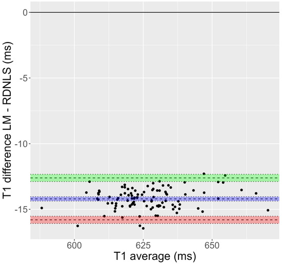
Figure 1.
Bland-Altman plot corresponding to Test 1 (inversion recovery, mouse data). It is evident that the T1 obtained by Bruker’s fit is greater than that derived from RD-NLS.
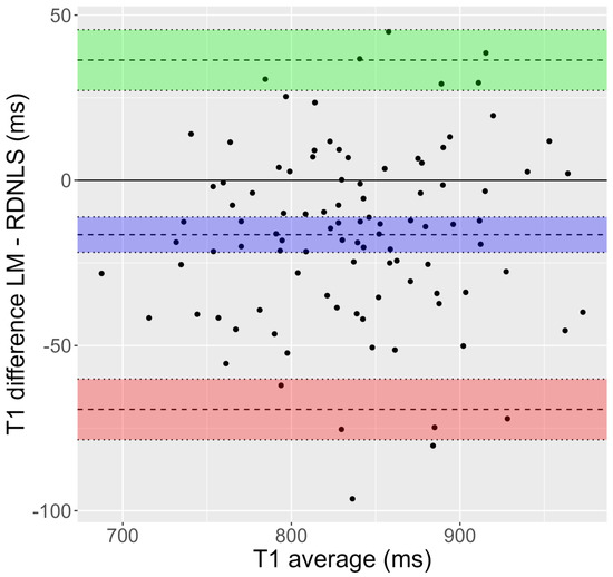
Figure 2.
Bland-Altman plot corresponding to Test 8 (inversion recovery, simulated human data). T1 values show a significant dispersion. Moreover, T1 obtained by Matlab’s fit (Lebenberg-Marquardt) is greater than the one attained by RD-NLS.
- The T1 fits (Tests 1–10) show many pixels in which error vs. T1 has more than one local minimum, in the 9–70% range. Having more than one local minimum means that a local search algorithm could get trapped in a local minimum which is not a global minimum (see Figure 3). This is not the case for the T2 fits (Tests 11–14), where error vs. T2 has only one local minimum.
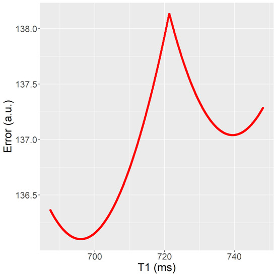 Figure 3. Fitting error (y) as a T1 (x) function after parameters A and B have been fitted. The T1 value obtained in fit (RD-NLS) was T1 = 696 ms, whereas the T1 value obtained in fit b (Matlab, Levenberg-Marquardt) was T1 = 740 ms. It corresponds to Test 2 (mouse data).
 - The Trel value obtained by the RD-NLS algorithm always corresponds to the global optimum.
- Comparing Bruker and Matlab fit versus RD-NLS for the T1 maps (Tests 1–10), the fit is different in a significant number of pixels, in the range of 5–97%. However, this is not true for the T2 maps (Tests 11–14).
Figure 1 and Figure 2 show Bland-Altman plots for Tests 1 and 8. Supporting Figures S1–S14 also show Bland-Altman plots for these tests. In addition, Table 4 shows bias and limits of agreement for all tests. In all cases, the differences refer to the relaxation time obtained using the algorithm used as a comparison minus the relaxation time obtained using the RD-NLS algorithm. As it is obvious from the results of these plots, the T1 values obtained in mouse data fitted with Matlab versus RD-NLS are quite similar for Tests 2–7. For Tests 8–10, the T1 values obtained in simulated data fitted with Matlab and RD-NLS show much more dispersion than in Tests 2–7. Besides, in Tests 8 and 9, Levenberg-Marquardt and Nelder-Mead fit gives a higher T1 value than RD-NLS fit, whereas no such difference appears in Test 10 (Split versus RD-NLS). Test 1 (mouse data) shows a clear distinction, with ISA fit giving a higher T1 value than RD-NLS fit. However, T2 values obtained in both fits are very similar for Tests 11–14 (phantom data).
Table 4.
Bias and limits of agreement from the tests. Bland-Altman plots corresponding to this table are given in Figure 1 and Figure 2, and in Figures S1–S14 in the supplementary materials.
Figure 3 illustrates an example of the fitting results for a specific pixel from Test 2, which involves using the Inversion Recovery technique to analyze mouse data. The plot in the figure represents the fitting error as a function of Trel after the linear parameters have been fitted. The plot shows two different fits, labeled as fit a and fit b, obtained using two different methods.
Fit a, obtained using the RD-NLS algorithm, corresponds to the global minimum, meaning it has the lowest fitting error among all the possible fits.
On the other hand, fit b, obtained using Matlab, reached a local minimum, meaning that the fitting error is greater than that of the global minimum. This indicates that the Matlab algorithm did not perform as well as the RD-NLS algorithm in fitting the data to the model. The local minimum could be caused by the algorithm getting stuck in a suboptimal solution rather than finding the global solution.
4. Discussion
A critical aspect of assessing the performance of a relaxation time fitting algorithm is the accuracy of its predictions, which can be quantified using the error between predicted and measured signal values. All fitting algorithms aim to minimize this error to achieve accurate and reliable relaxation time maps. Our results demonstrate that the RD-NLS algorithm outperforms the comparison algorithms regarding fit error, although the magnitude of improvement varies depending on the specific MRI dataset and signal model. It is noteworthy that we did not observe any instances where the RD-NLS algorithm was outperformed by the comparison algorithms. As shown in Figure 1, the difference in relaxation time values between algorithms can have a significant impact on tissue characterization. Therefore, the bias introduced by inaccurate relaxation time mapping could have implications for clinical diagnosis and treatment planning, underscoring the importance of developing and validating robust algorithms such as RD-NLS for accurate and reliable relaxation time mapping in MRI.
Figure 3 provides insight into the superior performance of the RD-NLS algorithm over the other tested algorithms and highlights the issue of bias in Trel values obtained from the fit. The “W” shape of the fitting error vs. Trel curve with multiple local minima can be observed for some pixels, as shown in Figure 3. The RD-NLS algorithm can find all such minima and choose the one that leads to the lowest error. In contrast, a local search algorithm may get stuck in a local minimum, depending on the starting conditions, which are known to be a critical issue when using this type of algorithm. In fairness, the authors attempted to find good starting conditions, but it is not always an easy task. For example, Figure 3 illustrates that for a particular pixel, the region between 680–760 ms is a good starting point for parameter T1. If the starting point is inappropriate, a local search algorithm may converge to a suboptimal solution and overestimate or underestimate T1. For example, if the starting point is T1 = 730 ms, a local search algorithm will converge to T1 = 740 ms, and this local search algorithm will, in this case, overestimate T1. However, if the starting point is T1 = 710 ms, a local search algorithm will converge to T1 = 696 ms, and this local search algorithm will find the correct T1 value. This example illustrates the importance of using appropriate algorithms and techniques in fitting image data to models, as the choice of algorithm can greatly impact the accuracy of the results. The RD-NLS algorithm provided a more accurate estimate of the relaxation time, while the Matlab algorithm reached a suboptimal solution. The choice of algorithm can greatly impact the accuracy of the results, and the RD-NLS algorithm eliminates the risk of failure to find the global optimum. Although the running time was not measured in this paper, high-speed implementations of the RD-NLS algorithm are available [30].
5. Conclusions
The examples presented in the study demonstrate that the RD-NLS algorithm outperforms other commonly used algorithms, such as Levenberg-Marquardt or Nelder-Mead, in fitting relaxation time maps. The study’s results suggest that the RD-NLS algorithm can provide a more accurate estimate of the relaxation time, resulting in a higher degree of accuracy in the relaxation time maps.
As seen in test 1, T1 maps fitted using different algorithms show differences in average T1, which can be as large as 14 ms. This shows that the choice of fitting algorithm can potentially affect T1 quantification.
The study’s authors recommend using the RD-NLS algorithm for obtaining relaxation time maps, as it is more effective than other algorithms in fitting image data to models. This algorithm can lead to more precise and accurate results, which is particularly important in medical imaging, where precise measurements are critical to the diagnosis and treatment of various conditions.
Additionally, the authors highlight that the RD-NLS algorithm has several advantages, such as that it is relatively simple to use, can provide solutions even in cases where the cost function has multiple local minima, and does not require initial estimates.
In conclusion, the use of the RD-NLS algorithm for obtaining relaxation time maps is highly recommended by the authors due to its superior performance in fitting image data to models.
Supplementary Materials
The following supporting information can be downloaded at: https://www.mdpi.com/article/10.3390/app13074083/s1, Figure S1: Bland-Altman plot corresponding to Test 1. It is evident that the T1 obtained by Bruker’s fit is greater than that obtained by RD-NLS. Figure S2: Bland-Altman plot corresponding to Test 2. T1 obtained by Matlab’s fit is slightly greater than the one attained by RD-NLS. Figure S3: Bland-Altman plot corresponding to Test 3. T1 obtained by Matlab’s fit is similar to the one obtained by RD-NLS. Figure S4: Bland-Altman plot corresponding to Test 4. T1 obtained by Matlab’s fit is similar to the one obtained by RD-NLS. Figure S5: Bland-Altman plot corresponding to Test 5. Note that the T1 obtained by Matlab’s fit is lower than the one obtained by RD-NLS. Figure S6: Bland-Altman plot corresponding to Test 6. T1 obtained by Matlab’s fit is similar to the one obtained by RD-NLS. Figure S7: Bland-Altman plot corresponding to Test 7. Note that the T1 obtained by Matlab’s fit is lower than the one obtained by RD-NLS. Figure S8: Bland-Altman plot corresponding to Test 8. The T1 values show an important dispersion. The results show that the T1 obtained by Matlab’s fit is greater than the one obtained by RD-NLS. Figure S9: Bland-Altman plot corresponding to Test 9. T1 values show an important dispersion. The figure shows that the T1 obtained by Matlab’s fit is greater than the one obtained by RD-NLS. Figure S10: Bland-Altman plot corresponding to Test 10. T1 values show an important dispersion. The T1 obtained by Matlab’s fit is similar to the one computed by RD-NLS. Figure S11: Bland-Altman plot corresponding to Test 11. T2 values show a very low dispersion, except for two outlier points. Note that the T2 calculated by Bruker’s fit is similar to the one determined by RD-NLS. Figure S12: Bland-Altman plot corresponding to Test 12. T2 values show a very low dispersion, except for one outlier point. The T2 attained by Matlab’s fit is almost similar to the one obtained by RD-NLS. Figure S13: Bland-Altman plot corresponding to Test 13. T2 values show a very low dispersion. The T2 calculated by Matlab’s fit is almost the same as the one determined by RD-NLS. Figure S14: Bland-Altman plot corresponding to Test 14. T2 values show a very low dispersion. Note the similarity between the T2 values obtained by Matlab’s and RD-NLS fits. Table S1: Summary of parameters used for Model I. They include parameters used in the RD-NLS algorithm, other algorithms, and the comparison of algorithms. Table S2: Summary of parameters used for Model II. They include parameters used in the RD-NLS algorithm, other algorithms, and the comparison of algorithms. Table S3: Summary of parameters used for Model III. They include parameters used in the RD-NLS algorithm, other algorithms, and the comparison of algorithms.
Author Contributions
Conceptualization, I.R., E.Y. and J.R.-C.; methodology, I.R., J.L.I.-G., E.Y., D.C. and J.R.-C.; software, I.R.; validation, I.R., J.L.I.-G., E.Y. and J.R.-C.; formal analysis, I.R. and J.L.I.-G.; investigation, I.R., J.L.I.-G., E.Y. and D.C.; resources, I.R. and D.C.; data curation, I.R. and D.C.; writing—original draft preparation, I.R. and J.L.I.-G.; writing—review and editing, I.R., J.L.I.-G., E.Y., D.C. and J.R.-C.; visualization, I.R. and J.L.I.-G.; supervision, I.R. and J.R.-C.; project administration, I.R.; funding acquisition, I.R., J.L.I.-G. and J.R.-C. All authors have read and agreed to the published version of the manuscript.
Funding
This work was supported by grants from Comunidad de Madrid (Grant S2017/BMD-3875), the Spanish Ministry of Science and Innovation (Grant PID2019-10656RJ-I00, PID2021-123238OB-I00 and PDC2021-121696-I00) and the European Union’s Horizon 2020 Research and Innovation Program, under the Marie Skłodowska-Curie grant agreement no. 823854 (INNOVA4TB). JRC received funding from the BBVA Foundation (Ayudas a Equipos de investigación científica Biomedicina 2018) and LaCaixa Foundation (HR20-00075). JRC received a grant from the Fundación contra la Hipertensión Pulmonar (2018).
Institutional Review Board Statement
The animal study protocol was approved by the Ethics Committee of Centro Nacional de Investigaciones Cardiovasculares (protocol code PA-60/12 and date of approval 8 January 2013).
Data Availability Statement
All the software and data, along with the instructions to run the tests, can be downloaded from https://github.com/ignrodri/rdnls (accessed on 15 March 2023) and is available for the general public. In addition, brain image data (mouse and human simulated) is available at openneuro.org.
Acknowledgments
The authors acknowledge Daniel Padro for providing some of the data used in this work and for helpful discussions. Part of the MRI studies was performed at the BioImaC (Centro de BioImagen Complutense) node of the ICTS (Infraestructuras Científicas y Técnicas Singulares) ReDIB.
Conflicts of Interest
The authors declare no conflict of interest.
References
- Kellman, P.; Hansen, M.S. T1-Mapping in the Heart: Accuracy and Precision. J. Cardiovasc. Magn. Reson. Off. J. Soc. Cardiovasc. Magn. Reson. 2014, 16, 2. [Google Scholar] [CrossRef]
- Ugander, M.; Bagi, P.S.; Oki, A.J.; Chen, B.; Hsu, L.-Y.; Aletras, A.H.; Shah, S.; Greiser, A.; Kellman, P.; Arai, A.E. Myocardial Edema as Detected by Pre-Contrast T1 and T2 CMR Delineates Area at Risk Associated with Acute Myocardial Infarction. JACC Cardiovasc. Imaging 2012, 5, 596–603. [Google Scholar] [CrossRef] [PubMed]
- Lescher, S.; Jurcoane, A.; Veit, A.; Bähr, O.; Deichmann, R.; Hattingen, E. Quantitative T1 and T2 Mapping in Recurrent Glioblastomas under Bevacizumab: Earlier Detection of Tumor Progression Compared to Conventional MRI. Neuroradiology 2015, 57, 11–20. [Google Scholar] [CrossRef]
- Truhn, D.; Sondern, B.; Oehrl, S.; Tingart, M.; Knobe, M.; Merhof, D.; Kuhl, C.; Thüring, J.; Nebelung, S. Differentiation of Human Cartilage Degeneration by Functional MRI Mapping-an Ex Vivo Study. Eur. Radiol. 2019, 29, 6671–6681. [Google Scholar] [CrossRef]
- Gracien, R.-M.; Nürnberger, L.; Hok, P.; Hof, S.-M.; Reitz, S.C.; Rüb, U.; Steinmetz, H.; Hilker-Roggendorf, R.; Klein, J.C.; Deichmann, R.; et al. Evaluation of Brain Ageing: A Quantitative Longitudinal MRI Study over 7 Years. Eur. Radiol. 2017, 27, 1568–1576. [Google Scholar] [CrossRef]
- Mariette, F.; Collewet, G.; Davenel, A.; Lucas, T.; Musse, M. Quantitative MRI in Food Science & Food Engineering. In Encyclopedia of Magnetic Resonance; Harris, R.K., Ed.; John Wiley & Sons, Ltd: Chichester, UK, 2012; p. emrstm1272. ISBN 978-0-470-03459-0. [Google Scholar]
- Bidhult, S.; Kantasis, G.; Aletras, A.H.; Arheden, H.; Heiberg, E.; Hedström, E. Validation of T1 and T2 Algorithms for Quantitative MRI: Performance by a Vendor-Independent Software. BMC Med. Imaging 2016, 16, 46. [Google Scholar] [CrossRef]
- Messroghli, D.R.; Moon, J.C.; Ferreira, V.M.; Grosse-Wortmann, L.; He, T.; Kellman, P.; Mascherbauer, J.; Nezafat, R.; Salerno, M.; Schelbert, E.B.; et al. Clinical Recommendations for Cardiovascular Magnetic Resonance Mapping of T1, T2, T2* and Extracellular Volume: A Consensus Statement by the Society for Cardiovascular Magnetic Resonance (SCMR) Endorsed by the European Association for Cardiovascular Imaging (EACVI). J. Cardiovasc. Magn. Reson. Off. J. Soc. Cardiovasc. Magn. Reson. 2017, 19, 75. [Google Scholar] [CrossRef]
- Salerno, M.; Kramer, C.M. Advances in Parametric Mapping with CMR Imaging. JACC Cardiovasc. Imaging 2013, 6, 806–822. [Google Scholar] [CrossRef]
- Taylor, A.J.; Salerno, M.; Dharmakumar, R.; Jerosch-Herold, M. T1 Mapping: Basic Techniques and Clinical Applications. JACC Cardiovasc. Imaging 2016, 9, 67–81. [Google Scholar] [CrossRef]
- Brown, R.W.; Cheng, Y.-C.N.; Haacke, E.M.; Thompson, M.R.; Venkatesan, R. Magnetic Resonance Imaging: Physical Principles and Sequence Design, 2nd ed.; John Wiley & Sons, Inc.: Hoboken, NJ, USA, 2014; ISBN 978-0-471-72085-0. [Google Scholar]
- Vlaardingerbroek, M.T.; den Boer, J.A.; Luiten, A. Magnetic Resonance Imaging: Theory and Practice; with a Historical Introduction by André Luiten; with 57 Image Sets; Physics and Astronomy online Library, 3rd ed.; Springer: Berlin/Heidelberg, Germany, 2010; ISBN 978-3-642-07823-1. [Google Scholar]
- Bernstein, M.A.; King, K.F.; Zhou, X.J. Handbook of MRI Pulse Sequences; Elsevier Academic Press: Amsterdam, The Netherlands, 2004; ISBN 978-0-12-092861-3. [Google Scholar]
- Deoni, S.C.L.; Rutt, B.K.; Peters, T.M. Rapid Combined T1 and T2 Mapping Using Gradient Recalled Acquisition in the Steady State. Magn. Reson. Med. 2003, 49, 515–526. [Google Scholar] [CrossRef]
- Deoni, S.C.L.; Peters, T.M.; Rutt, B.K. Determination of Optimal Angles for Variable Nutation Proton Magnetic Spin-Lattice, T1, and Spin-Spin, T2, Relaxation Times Measurement. Magn. Reson. Med. 2004, 51, 194–199. [Google Scholar] [CrossRef] [PubMed]
- Pirastru, A.; Chen, Y.; Pelizzari, L.; Baglio, F.; Clerici, M.; Haacke, E.M.; Laganà, M.M. Quantitative MRI Using STrategically Acquired Gradient Echo (STAGE): Optimization for 1.5 T Scanners and T1 Relaxation Map Validation. Eur. Radiol. 2021, 31, 4504–4513. [Google Scholar] [CrossRef] [PubMed]
- Haacke, E.M.; Chen, Y.; Utriainen, D.; Wu, B.; Wang, Y.; Xia, S.; He, N.; Zhang, C.; Wang, X.; Lagana, M.M.; et al. STrategically Acquired Gradient Echo (STAGE) Imaging, Part III: Technical Advances and Clinical Applications of a Rapid Multi-Contrast Multi-Parametric Brain Imaging Method. Magn. Reson. Imaging 2020, 65, 15–26. [Google Scholar] [CrossRef] [PubMed]
- Ramos-Llorden, G.; Vegas-Sanchez-Ferrero, G.; Bjork, M.; Vanhevel, F.; Parizel, P.M.; San Jose Estepar, R.; den Dekker, A.J.; Sijbers, J. NOVIFAST: A Fast Algorithm for Accurate and Precise VFA MRI Mapping. IEEE Trans. Med. Imaging 2018, 37, 2414–2427. [Google Scholar] [CrossRef] [PubMed]
- Levenberg, K. A Method for the Solution of Certain Non-Linear Problems in Least Squares. Q. Appl. Math. 1944, 2, 164–168. [Google Scholar] [CrossRef]
- Marquardt, D. An Algorithm for Least-Squares Estimation of Nonlinear Parameters. SIAM J. Appl. Math. 1963, 11, 431–441. [Google Scholar] [CrossRef]
- Nelder, J.A.; Mead, R. A Simplex Method for Function Minimization. Comput. J. 1965, 7, 308–313. [Google Scholar] [CrossRef]
- Golub, G.H.; Pereyra, V. The Differentiation of Pseudo-Inverses and Nonlinear Least Squares Problems Whose Variables Separate. SIAM J. Numer. Anal. 1973, 10, 413–432. [Google Scholar] [CrossRef]
- Nonlinear Data-Fitting—MATLAB & Simulink—MathWorks. Available online: https://www.mathworks.com/help/optim/ug/nonlinear-data-fitting-example.html#datdemo-4 (accessed on 6 November 2020).
- Barral, J.K.; Gudmundson, E.; Stikov, N.; Etezadi-Amoli, M.; Stoica, P.; Nishimura, D.G. A Robust Methodology for in Vivo T1 Mapping. Magn. Reson. Med. 2010, 64, 1057–1067. [Google Scholar] [CrossRef]
- Messroghli, D.R.; Radjenovic, A.; Kozerke, S.; Higgins, D.M.; Sivananthan, M.U.; Ridgway, J.P. Modified Look-Locker Inversion Recovery (MOLLI) for High-Resolution T1 Mapping of the Heart. Magn. Reson. Med. 2004, 52, 141–146. [Google Scholar] [CrossRef]
- Nekolla, S.; Gneiting, T.; Syha, J.; Deichmann, R.; Haase, A. T1 Maps by K-Space Reduced Snapshot-FLASH MRI. J. Comput. Assist. Tomogr. 1992, 16, 327–332. [Google Scholar] [PubMed]
- Kwan, R.K.; Evans, A.C.; Pike, G.B. MRI Simulation-Based Evaluation of Image-Processing and Classification Methods. IEEE Trans. Med. Imaging 1999, 18, 1085–1097. [Google Scholar] [CrossRef] [PubMed]
- Collins, D.L.; Zijdenbos, A.P.; Kollokian, V.; Sled, J.G.; Kabani, N.J.; Holmes, C.J.; Evans, A.C. Design and Construction of a Realistic Digital Brain Phantom. IEEE Trans. Med. Imaging 1998, 17, 463–468. [Google Scholar] [CrossRef] [PubMed]
- Bland, J.M.; Altman, D.G. Statistical Methods for Assessing Agreement between Two Methods of Clinical Measurement. Lancet Lond. Engl. 1986, 1, 307–310. [Google Scholar]
- Kim, Y.-C.; Kim, K.R.; Lee, H.; Choe, Y.H. Fast Calculation Software for Modified Look-Locker Inversion Recovery (MOLLI) T1 Mapping. BMC Med. Imaging 2021, 21, 26. [Google Scholar] [CrossRef]


Disclaimer/Publisher’s Note: The statements, opinions and data contained in all publications are solely those of the individual author(s) and contributor(s) and not of MDPI and/or the editor(s). MDPI and/or the editor(s) disclaim responsibility for any injury to people or property resulting from any ideas, methods, instructions or products referred to in the content. |
© 2023 by the authors. Licensee MDPI, Basel, Switzerland. This article is an open access article distributed under the terms and conditions of the Creative Commons Attribution (CC BY) license (https://creativecommons.org/licenses/by/4.0/).