Abstract
The use of boundary elements in the analysis of exterior acoustic problems poses challenges at specific frequencies, since fictitious eigenfrequencies may arise at the internal resonances of cavities, leading to inaccurate results or even unstable behavior. To filter out these fictitious eigenfrequencies, a scheme based on the combined Helmholtz integral equation formulation (CHIEF) can be used to prevent the so-called non-uniqueness problem, although it requires additional equations and points. The BEM formulation final accuracy will, however, depend on the correct choice of these points. Here, a strategy to help in defining good approximations for the position and number of such points is proposed, based on an optimization process which maximizes the system matrix’s smallest singular value. The accuracy of the method for exterior radiation problems is investigated using different examples. With low computational cost and simple implementation, the two proposed algorithms automatically circumvent the non-uniqueness problem, aiding the implementation of more stable BEM codes.
1. Introduction
The boundary-element method (BEM) can be used to analyze and solve dynamic acoustic problems both in the frequency domain (FD) and in the time domain (TD). Both the BEM-FD and the BEM-TD suffer from numerical instabilities related to the (numerical) resolution of both the Kirchhoff–Helmholtz integral boundary equation and its normal derivative [1]. Investigations into the cause of such instabilities can be found in [2,3]. In general, it can be understood as an oscillation generated by the numerical solution procedure, where the coupling between the incident field and the internal resonance modes does not entirely vanish [4]. In this case (i.e., by understanding it as an eigenvalue boundary problem), fictitious eigen-frequencies arise due to the problem’s resonant frequencies, resulting in spurious oscillations that generate unreliable results. Many publications have addressed the described problem, and some recent works mention different alternatives to circumvent the problem, for example the recent review paper by Kirkup [5] or the overview presented by Marburg [6], which identify the relevant problem of irregular frequencies in external BEM models and refer to the main alternatives to address and solve that issue.
One of the first approaches to deal with this problem in the frequency domain was presented by Schenck [5], who proposed the combined Helmholtz integral equation formulation (CHIEF), consisting of using the Helmholtz integral equation in the boundary combined with additional compatible equations, formulated from the integral equation for some internal points, external to the infinite domain and conveniently located to improve the conditioning of the final matrix. A popular alternative strategy is the Burton and Miller approach, initially formulated in [7], which combines the classical BEM integral equation and its normal derivative and, when coupled together by a specific coefficient, allows the definition of stable solutions at the fictitious frequencies. Although this is a well-accepted method, there are still discussions regarding its application, such as in [6] and [8]. Some authors [6] even mention that half of the references on the method are incorrect due to an erroneous coupling coefficient. In other works [9], complementary strategies have been devised to improve the behavior of the method.
Alternative works can be found in the literature addressing the stability of the BEM for external problems using other techniques. Engleder and Steinbach [10], for instance, formulated and analyzed a modified boundary-element method for Dirichlet conditions, showing that it was stable for all wave numbers, thus avoiding the unstable behavior at irregular frequencies. In contrast to other existing approaches, the proposed method relies on the use of boundary integral operators which are already available in standard boundary-element methods. Therefore, the additional effort in the implementation is neglectable. Mingsong et al. [11] addressed the problem using the so-called Closed Virtual Impedance Surface Method (CVIS), and stated that the technique allowed the virtual elimination of the effects of these fictitious frequencies. Klaseboer et al. [12] proposed the use of a modified Green’s function and presented results showing that it can indeed remove certain fictitious frequencies. However, the authors indicated that their results were an initial proof of concept for the method, requiring further developments.
In spite of existing alternatives, due to its simplicity, the CHIEF method is still one of the most widely used techniques to circumvent non-uniqueness problems at irregular frequencies of BEM models and also has the potential to be applied to other techniques. Indeed, recent works confirm its use and effectiveness. Panagiotopoulos et al. [13] used CHIEF points to stabilize a BEM formulation with Krylov subspace recycling to improve efficiency, indicating a rule of thumb for using a number of CHIEF points which is about 5% of the total number of nodes. Barbarino and Bianco [14] used a fast multipole BEM for aero-acoustic problems, using the CHIEF method to avoid irregular frequencies. In their proposal, the CHIEF point selection for 3D problems is automatized while still random, being linked to a multi-level octree decomposition, together with a point-in-polyhedron algorithm; the thumb rule of 5% of CHIEF points is also mentioned in this work. In a very recent paper, Wu et al. [15] also showed the applicability of the CHIEF method to recent meshless techniques, particularly to the singular boundary method (SBM). In this work, the so-called modified SBM is indeed an extension of the method by incorporating CHIEF points to avoid unstable results at specific frequencies, using a so-called self-regularization technique. These authors also compared their technique with a Burton–Miller SBM and indicated that the CHIEF method can lead to more accurate results in the tested problem.
Following the given references, the classic CHIEF method is not only a relevant technique for the BEM itself but is also useful as a complement in more recent methods. For the latter, the principle of application is exactly the same as for the BEM, and so the same exact problems are expected to occur, in particular the definition of convenient location and number of CHIEF points for each problem. This so-called “convenient location” of CHIEF points is not easily established, and a bad selection of these point locations may cause the procedure to fail or lead to less accurate results. Wu et al. [16] proposed a CHIEF-block idea to enforce constraints in a weighted residual sense over a small region. However, if the CHIEF point is located over or near the nodal line of its corresponding mode, it may not provide a valid constraint [17,18]. To overcome this problem, Chen et al. [8,9] presented an analytical study to select a valid number of CHIEF points and their positions for circular cavities by using circulants. However, their discussions were limited to circular configurations, and its extension to general geometrical formats is not trivial. After that, Chen et al. [19] proposed a criterion in selecting the minimum number of CHIEF points and their positions by testing the orthogonal condition between the influence row vector and the right unitary vector, proving a further advancement on the topic. On the other hand, Bartolozzi et al. [20] suggested that the best efficiency was achieved by the random selection of CHIEF points.
In this paper, a method based on an optimization process, which maximizes the smallest singular value of the system matrix, is considered to formulate a criterion for selecting the number of CHIEF points as well as their locations. The method is here applied to 2D problems, although its extension to higher dimensional problems should not pose any difficulties. The paper is organized as follows: first, the general formulation of the BEM is given for acoustic problems; there follows a brief description of the CHIEF method; next, the algorithms that are proposed and analyzed in this paper are described; and, finally, numerical examples are presented and discussed.
2. Materials and Methods
2.1. The Boundary-Element Method
Consider an infinite 2D acoustic domain Ω, containing an inclusion with a regular and smooth boundary defined as . Externally to this inclusion, there is the domain where the acoustic field exists, defined as , while the interior of the inclusion is defined as . This scenario is represented in Figure 1.
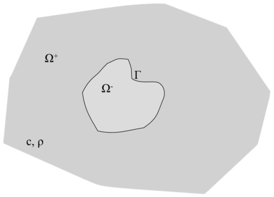
Figure 1.
General scheme of the analyzed problem with a cavity inside an infinite homogeneous acoustic medium.
Assuming that in there is a compressible and homogeneous medium with sound velocity , the linearized wave equation in the time domain in terms of acoustic pressure is written through:
Considering that the waves are produced by harmonic periodic vibrations in time, the response will also be periodic through the propagation domain of the fluid; thus, the acoustic pressure can be written as:
where is the angular frequency of vibration and response, is the representation of the imaginary part of the complex number and t is the time of analysis. Coupling Equation (1) to Equation (2), the differential equation that governs the steady state of linear acoustics can be obtained. This is defined by the Helmholtz equation, which may be written as:
where is the wave pressure at point x in the exterior acoustic field, is the Laplacian operator, and is the wave number. The boundary value problem (BVP) is defined by Dirichlet and Neumann conditions, respectively:
where is the normal unitary vector at defined as , pointing outwards of the domain, is the acoustic flow, and is the acoustic pressure, both prescribed at .
Rewriting Equation (3) as the Kirchhoff–Helmholtz boundary integral equation, the following is obtained:
where is the fundamental solution for the Helmholtz equation and stands for its normal derivative, defined as:
where , and e are the Hankel functions of the second type and order zero and one, respectively.
This work uses constant elements, so in Equation (6), is a constant that can be defined as:
By discretizing Equation (6) through boundary collocation points, it is possible to generate a system of algebraic equations, where, for each collocation point, the integration of all the boundary elements (NE) is carried out, generating NE linearly independent equations:
where:
The solution of this system of equations, for each wave number (), presents, in general, a unique acoustic pressure and flow response.
2.2. The CHIEF Method
It is known that the application of the described BEM technique for solving external acoustic problems (infinite media) may produce a non-unique response [4]. The resonance modes observed within the domain are on the imaginary axis and, theoretically, would never be excited by the external incident field [21]. However, it has been observed that the internal resonance modes do not vanish completely, in such a way that numerical error occurs when the vibration frequencies of the infinite domain approach the natural frequencies of the internal body .
By analyzing the boundary eigenvalue problem, if the resonance modes inside the domain are within the analyzed frequency range, it can be noticed that spurious or fictitious eigenfrequencies arise. In case of instability, the results for high frequencies begin to oscillate with exponentially increasing amplitude [21]. In order to solve this problem and to “filter” such eigenfrequencies, the combined Helmholtz integral equation formulation (CHIEF) technique can be used, which is the focus of this paper.
The purpose of the CHIEF formulation is to minimize the error by enforcing additional constrains. The technique consists of adding collocation points outside the domain of analysis (the so-called CHIEF points), and through these new points adding new equations to the algebraic system. If the BEM collocation points are on the body boundary, the idea is that the CHIEF points are outside the body of analysis, in the internal domain itself. Thus, each additional equation has the form:
which corresponds to enforcing null p values at specific points in . Thus, by defining , the system defined by Equation (10), in matrix form, would result in:
The final non-square system of equations can then be solved using a least-squares technique.
2.3. Proposal for the Location of the CHIEF Points
Although, in principle, the proposed strategy is very simple to implement (and may be very efficient), defining where to place CHIEF additional points is not a trivial task, especially if complex geometries are regarded.
To help define the location of these points, it is important to understand that non-unique responses of the system occur due to its ill-conditioning. An indicator of this behavior is the occurrence of small singular values (or a large relationship between the largest and the smallest singular values) or a large condition number of the matrix. Taking this into account, a strategy based on the addition of CHIEF points within , which allows for this ill-conditioning to be reduced, can be developed by optimizing the location of these points based on a parameter that allows this behavior to be represented.
The proposed strategy consists of first computing the system matrix using the standard BEM formulation, without any CHIEF points. The possibility of ill-conditioning is then evaluated by means of the evaluation of the smallest singular value (SV) of the matrix and comparing it with a given limit. If this smallest SV is below the specified limit, a CHIEF point is added at a random location, and after this an optimization routine is applied, finding the position of the CHIEF point which maximizes the smallest SV. It should be noted that inside the optimization algorithm only an update of a very limited number of lines (equal to the number of CHIEF points) in the system matrix is required, and the rest of the matrix remains unchanged. After optimization, if the SV limit has been reached, the procedure stops; otherwise, optimization is performed once again with one additional point, and the process goes on until either the SV limit has been reached or a maximum number of CHIEF points has been added. Figure 2 presents a flowchart illustrating this procedure.
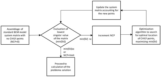
Figure 2.
Flowchart of the proposed algorithm.
In the present work, the implementation of the whole process is performed using MATLAB R2022b, and the optimization algorithm makes use of the “fmincon” function from the Optimization Toolbox, choosing the “interior point” with a maximum of 100 iterations. Two different implementations of the algorithm have been tested:
- ALG1—For each new set of CHIEF points, all the points are optimized simultaneously (e.g., if a 2nd point needs to be added, a new optimization is performed for both points together);
- ALG2—After each optimization, the new optimized point position is fixed and kept for the next step (e.g., if a 2nd point needs to be added, only the new point’s position is optimized, and the first point is kept at the previously determined position).
It should be noted that, for both algorithms, and according to Figure 2, the inclusion of CHIEF points only occurs when the smallest SV is below a given threshold, which allows for the original BEM response (i.e., with no CHIEF points) to be kept in all other situations. In addition, the number of CHIEF points is increased by one at a time, thus keeping the number of additional constraints to a minimum level. It will be shown later in this work that the smallest SV of the matrix has a relationship with the error of the calculated solution, and the higher its value, the lower the global error.
3. Numerical Experiments
3.1. Case 1—Radiating Circular Cavity
The first test case analyzed here (which is illustrated in Figure 3) corresponds to a circular cavity with a unit radius, embedded within a homogeneous acoustic medium.
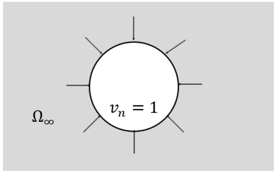
Figure 3.
Schematic representation of the first test case, with a circular cavity subject to a unit particle velocity throughout its boundary.
The host medium allows a propagation velocity of 340 m/s and has a density of 1.21 kg/m3. Along the boundary, a unit particle velocity is imposed as , and for this case an analytical solution can be derived, assuming the form:
where
and is the unitary particle velocity imposed at , with being the cylinder radius. In addition, and stand for the first kind Bessel function of zero and first order, respectively, whereas and are the second kind Bessel function of zero and first order, respectively, and stands for the distance of the point of analysis to the center of the cavity. In this case, the acoustic response is computed at a distance of 1.8 m from the center of the cavity, for frequencies between 5 and 500 Hz, and its real and imaginary parts are depicted in Figure 4b. In Figure 4c, the absolute pressure value, analytically calculated and using the BEM, is displayed, using a discretization with 63 boundary elements for the mesh (see Figure 4a for this adopted discretization). From these results, it is clear that a good match is obtained throughout the referred frequency range, except for some specific frequencies, in which it is possible to observe large deviations.
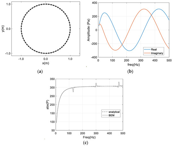
Figure 4.
Test case with a circular cavity with prescribed particle velocity: (a) BEM discretization with 63 constant elements; (b) real and imaginary parts of the analytical solution; (c) absolute value of the pressure solution considering analytically and numerically (with the BEM) computed responses.
Figure 5a illustrates the relative errors of the BEM results, together with the smallest SV of the BEM matrix, and Figure 5b shows the reciprocal of the matrix condition number (computed using MATLAB’s “rcond” command). Observing these plots, the three error peaks are quite evident, occurring at frequencies around 130, 300 and 470 Hz, for which relative errors reaching 10% can be seen. In both Figure 5a,b, it can be seen that these frequencies coincide with those describing dips in the smallest SV and “rcond” curves, indicating that these errors are associated with the ill-conditioning of the system. However, it should be noted that such dips also occur at other frequencies, for which no error increase is registered. The conventional approach of adding CHIEF points to stabilize the response that has been initially used by introducing one, two or three CHIEF points located randomly inside the cavity.
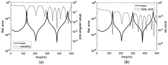
Figure 5.
BEM relative error and (a) smallest singular value of the BEM matrix; (b) reciprocal of the condition number of the BEM matrix.
Results for those cases are represented in Figure 6a–c, in which it is possible to observe that a significant improvement of the error is attained at the previously mentioned frequencies. The error improvement is, however, non-uniform throughout the frequency domain, and significant oscillations occur from frequency to frequency. Indeed, at some points the CHIEF points seem to originate a small degradation of the response, even when three points are used. The smallest SV is also represented in each plot, and it can be seen that the addition of the first CHIEF point significantly improves the first dip in that curve but only slightly affects the remaining ones. In particular, the error peak at 470 Hz still occurs, although slightly attenuated. As more points are added, the smallest SV curve improves, but dips are still clearly visible, indicating that a more stable matrix is obtained, in particular at higher frequencies.
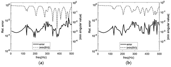
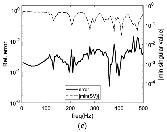
Figure 6.
BEM relative error with one (a), two (b) and three (c) CHIEF points. The smallest singular value for each case is also plotted.
To better understand the influence of the CHIEF point position, the colormaps in Figure 7 illustrate the smallest SV computed for the matrix as a function of the position of one CHIEF point. Results for six frequencies are illustrated, including those where error peaks have been identified and other frequencies for which a dip in the smallest SV curve occurs but is not associated with any error. It is interesting to note that for the first three presented plots (see Figure 7a–c), there is a strong dependence of the smallest SV on the position of the CHIEF point. Moreover, for the two higher frequencies (i.e., 300 and 470 Hz), there are regions where the collocation of one CHIEF point can be totally ineffective (keeping a very small value of the SV). It is also interesting to note that for the other three illustrated frequencies (see Figure 7d–f), a completely different behavior occurs, and there is almost no dependence of the smallest SV on the position of the CHIEF point. Indeed, these results are in line with the expected behavior, with the first three frequencies corresponding to fictitious eigenvalues of the problem, for which non-unique responses are obtained, and the other three just being associated with a more regular behavior of the BEM and not specifically with that same type of non-unique response.
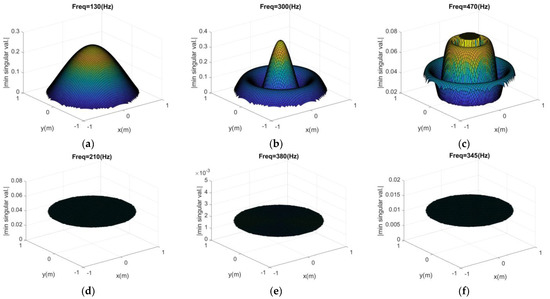
Figure 7.
Smallest singular value of the BEM matrix as a function of the position of one CHIEF point: (a–c) correspond to frequencies where simultaneously an error peak in the BEM model and a minimum in the singular value curve occur (see Figure 4a); (d–f) correspond to frequencies where no error peak occurs in the BEM model, but a minimum in the singular value curve occurs.
The proposed optimization algorithms have been applied to this test case, and the corresponding results are depicted in Figure 8a–d, considering a threshold of min(SV) > 0.1 for both algorithms. Figure 8a,c illustrate the relative error and the smallest SV curve registered for ALG1 and ALG2, while Figure 8b,d show the number of CHIEF points added during the optimization process. In both cases, min(SV) > 0.1 was attained with a small number of points, and the smallest SV curves are clearly more regular than when random points are used, without evident dips. The global error level is well controlled, particularly at higher frequencies, and no relevant peaks are observed. It is important to emphasize that CHIEF points are only used in a very limited number of frequencies (only when min(SV) > 0.1), and the used number of points depends on the specific frequency being analyzed. For the lower frequencies, typically one or two points are sufficient for both algorithms, while some of the higher frequencies require three or even four optimized CHIEF points. ALG2 seems to have a trend of requiring more points than ALG1 at the higher frequencies, which is in accordance with the expected behavior for these algorithms. Indeed, ALG2 independently optimizes one point at a time (point 2 is optimized only after point 1 is fixed, and so on), and as so its final point distribution is sub-optimal by nature. ALG1, on the other hand, optimizes the position of all points simultaneously, allowing a more effective search for the optimal distribution. However, ALG1 typically has a larger number of variables involved in the optimization, rendering a slower process. For example, considering the frequency of 470 Hz, both ALG1 and ALG2 require three CHIEF points for reaching the target smallest SV, but the computational effort time required by ALG1 is around 3.5 times higher. Even for 415 Hz, for which ALG1 only needs two points and ALG2 requires four points, ALG2 is 2 times faster. Importantly, the optimization process requires estimation of derivatives with respect to each variable at each iterative step until optimality is reached, so its computational effort is heavily dependent on the number of variables involved. Indeed, since only the x and y position of the additional CHIEF point are involved at each iteration of ALG2, the required computations are significantly reduced, and the algorithm reaches the optimal position of each additional point much quicker.
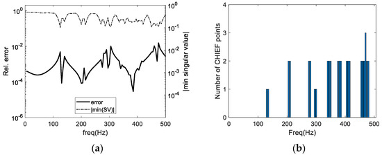
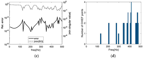
Figure 8.
Results computed using the proposed algorithms: (a,c) show the relative error and smallest singular value and (b,d) show the number of CHIEF points used at each frequency. (a,b) refer to algorithm ALG1, and (c,d) to algorithm ALG2.
Figure 9 illustrates results from both algorithms when different target values are set for the smallest SV, namely 0.05, 0.10, 0.20 and 0.30, considering a maximum of 10 CHIEF points, in terms of relative errors (Figure 9a1,b1) and of the smallest SV (Figure 9a2,b2). It is clear from these plots that limiting the value of the smallest SV has the effect of better controlling the registered error peaks, which tend to decrease when this limit is set to higher values. This occurs for both algorithms and gives a good indication about the interest of this approach in tackling the non-uniqueness problem occurring when the BEM is used for external problems. A sample point distribution for both algorithms and for a frequency of 470 Hz is shown in Figure 10, with six points being used in ALG1 to attain min(SV) > 0.3 and 10 points being required in ALG2 for the same purpose. Notably, in the case of ALG1, the locations of all point positions are optimized simultaneously, and so a more efficient control of the smallest SV is attained with far fewer points although at the expense of a higher computational cost than for ALG2.

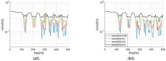
Figure 9.
Relative error (a1,b1) and smallest singular value (a2,b2) computed for the two algorithms ALG1 (a1,a2) and ALG2 (b1,b2), considering different acceptable values for min(SV) of 0.05, 0.1, 0.2 and 0.3. The same color pattern is used for all figures.
Figure 10.
Final position of the CHIEF points after the optimization procedure considering min (SV) > 0.3: (a) ALG1, requiring six points; (b) ALG2, requiring 10 points.
3.2. Case 2—Radiating Irregular Body
A second test case has been set up with the geometry depicted in Figure 11. For this case, an irregular boundary has been defined, following Equation (17):
where (r, θ) refers to the coordinates of the boundary points in cylindrical coordinates. Along this boundary, a unit particle velocity is imposed. The system is discretized using 100 constant boundary elements.
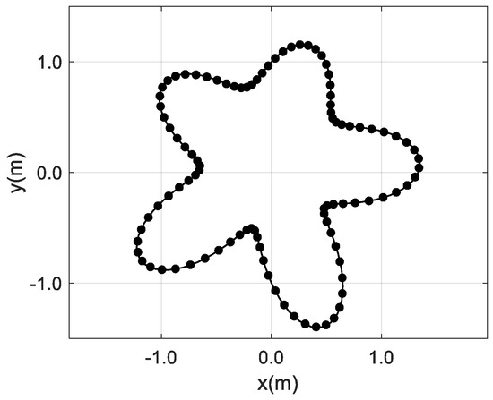
Figure 11.
Geometry of the second test problem, considering a flower-shaped domain with unit particle velocity along its boundary.
In Figure 12a, the computed solution using the standard BEM formulation shows the calculated absolute acoustic pressure, together with the smallest SV of the BEM matrix. As in the previous test case, the pressure curve exhibits a very irregular shape, with sharp peaks and dips that indicate an irregular behavior of the BEM that may be associated with non-unique solutions of the system of equations. The smallest SV curve also exhibits pronounced dips at almost all of those frequencies, a behavior indicating that, once more, a relationship between the occurrence of very low SVs and non-unique solutions of the BEM system exists, even in a stronger form than in the previous example.
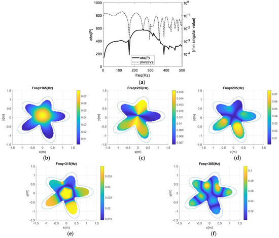
Figure 12.
(a) BEM response for the second test case, and (b–f) color maps of the minimum singular value of the system matrix when one CHIEF point is considered for different frequencies.
To assess the method’s behavior with the addition of a CHIEF point at some of these irregular frequencies, calculations were performed to observe the smallest SV of the system as a function of the position of this CHIEF point. Figure 12b–f illustrate this behavior for frequencies of 165, 255, 295, 315 and 385 Hz (for which an irregular behavior is observed), in the form of color maps, where lighter (yellow) shades indicate positions for which the existence of a CHIEF point will lead to higher values of the smallest SV (i.e., better conditioning), while blue shades indicate the opposite behavior. It is clear from these figures that there is a very strong dependence of the smallest SV from the position of the CHIEF point, a fact that has also been observed in the first test case but that is even more evident here. Indeed, for each analyzed frequency, there are significant parts of the analyzed space for which the collocation of a CHIEF point will have a very limited effect, an observation that indicates that the use of an optimization algorithm to assist the selection of the position of this point may be of great interest. At some specific positions, the effect of the introduction of an internal CHIEF point may be almost negligible, as is the case of the darker shades of blue in all the five figures.
In Figure 13, results are presented for this test case considering different situations. In the left column, results considering one, two or three randomly positioned points are illustrated, and, in the right column, the corresponding results considering the proposed algorithm are presented. In this last case, the number of used CHIEF points may vary between 0 and the maximum number allowed during the optimization process, which can be one (Figure 13b1), two (Figure 13b2) or three (Figure 13b3). To avoid a lengthy presentation of results, only ALG1 will be addressed here, but similar findings are also seen for ALG2.
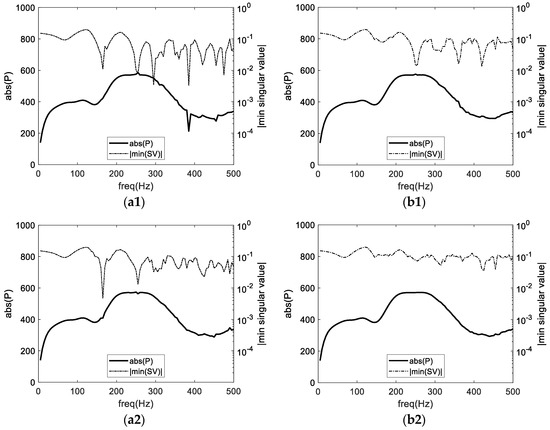
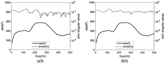
Figure 13.
Response computed for the second test problem, considering either (a1–a3) fixed or (b1–b3) optimized CHIEF point positions, for one (a1,b1), two (a2,b2) or three (a3,b3) points. For the optimized case, this number of points is the maximum considered in the optimization process.
By observing the presented results, it becomes quite clear that, in all cases, the use of the proposed optimization algorithm leads to a smoother solution curve than the use of random points. As a matter of fact, the results show that with just one CHIEF point, the irregular character of the solution curve is still very clear if a random CHIEF point is considered, with some spikes still being observable in many of the frequencies previously identified for the BEM solution, although with smaller amplitudes (for the frequency of 385 Hz, this spike is still quite pronounced, and almost no difference can be seen in relation to that of the classical BEM solution). As for the smallest SV curve, pronounced dips are still visible at many of those frequencies, further indicating that the addition of a randomly located CHIEF point may not be very effective. On the other hand, when the position of the CHIEF point is optimized, a smoother curve is obtained, and most of the spikes appear to be filtered by the optimization of that point’s location. Nevertheless, at high frequencies some irregularity is still observed and can be associated with lower values of the smallest SV, as seen in the same plot. By adding an additional point, the behavior seems to improve both for the optimized and for the non-optimized case, although it is clear that the optimization of these positions leads to an even smoother curve than before, with the smallest SV curve being shifted up at higher frequencies as well. Finally, by optimizing considering a maximum of three points, a very good response is registered. Figure 14 shows the number of points used at each frequency, revealing that indeed three points were required just at higher frequencies to control the system’s conditioning to a desired level. When no optimization is performed, even considering three randomly distributed CHIEF points, significant and visible irregularities may still be evident in the curve, mostly at high frequencies. Indeed, this second test case clearly shows that it can be quite challenging to choose good positions for the CHIEF points when a complex geometry is analyzed.
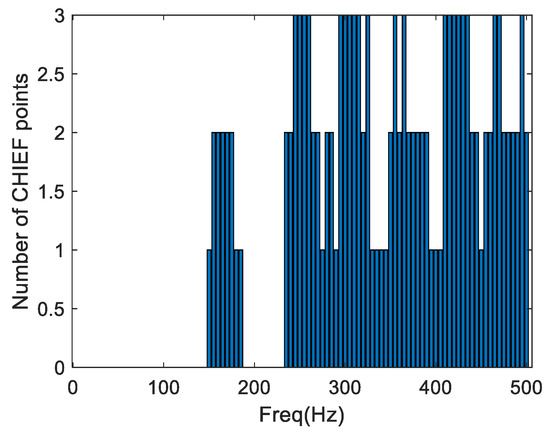
Figure 14.
Number of CHIEF points considered for each frequency, when the optimization was performed for a maximum of three CHIEF points.
For some additional insights regarding the effect of the random and optimized approaches, Figure 15 presents a detailed view of the response around one of the irregular frequencies (i.e., 255 Hz), considering the classical BEM, a random CHIEF point generation and the proposed optimization approach. It is evident that the classical BEM result has a dip and a peak around 253 Hz, diverging from the smooth trend of the response. Using one or two random CHIEF points may help to reduce this behavior, but it may still be not sufficient to provide appropriate results. Optimizing the position of these points, on the other hand, turns the curve quite smooth, correcting the non-uniqueness of the response.
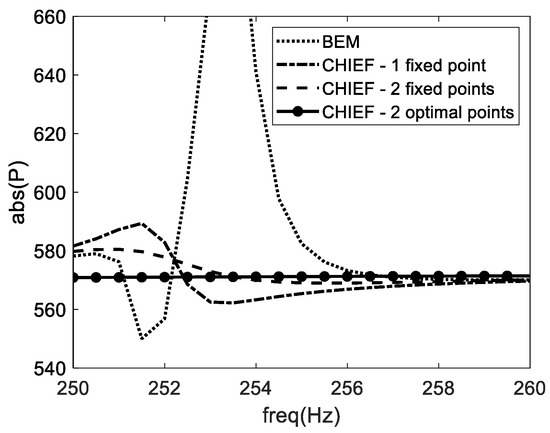
Figure 15.
Detail of the response at frequencies around 255 Hz, considering the BEM, one fixed CHIEF point, two fixed CHIEF points and two optimized CHIEF points.
Finally, Figure 16 presents the response at the frequency of 253 Hz, where the higher error peak was observed in Figure 15, computed using both ALG1 and with random point generation. The real and imaginary parts of the response are shown for different numbers of CHIEF points, ranging from 0 to 10. In both parts of the response, the results computed using ALG1 are clearly more stable, and the algorithm seems to be able to select a good position of the CHIEF points that minimizes oscillations of the response. This is particularly true for the real part of the response, which seems to stabilize after one point is introduced. Figure 16c1–c4 shows the distribution of optimal points for one, two, three and six CHIEF points, for the same frequency of 253 Hz. Since the algorithm optimizes all points simultaneously, different points are obtained for each case, and no common positions can be identified between the presented cases; additionally, the points seem to be placed mostly at positions where higher values of the smallest SV for one point were registered in Figure 12c (yellow shades). Observing Figure 16a,b, it can be seen that when random points are used, both the real and the imaginary parts of the response seem to be much less stable and tend to vary more significantly with the variation of the number of points, and even after introducing six CHIEF points there still seems to be some visible change of the imaginary part of the response. It should be noted that this response is for a single randomization of points and so will change from case to case. This contrasts with the case in which optimized positions of the CHIEF points are chosen, for which almost stable responses are seen with just two points, even for the imaginary part.
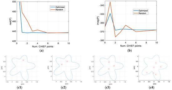
Figure 16.
Real (a) and imaginary (b) parts of the response calculated for different numbers of CHIED points using ALG1 and random point generation and positions of the CHIEF points (c1–c4) for one, two, three and six points after optimizations are represented.
To conclude this section, it is important to emphasize that the presented results indicate a good behavior of the proposed strategy, both in terms of the identification of the need for using CHIEF points and for the definition of their optimal locations. Even for the more complex shape of Case 2, smooth and stable results were reached with a limited number of CHIEF points, which were adaptively chosen for each tested frequency; in many cases, since the smallest SV was large enough, the algorithm introduced no CHIEF point at all, and this option proved to be adequate, still providing good results. These observations can be quite useful in the context of engineering applications, for which complex shapes are frequently used and for which the good choice of CHIEF point position can be a non-trivial task. The authors stress that the introduction of the algorithm in existing codes can be simple, and this can be a helpful addition for the users of BEM codes in engineering applications.
4. Final Remarks
The present paper revisits the topic of irregular frequencies that occur in exterior acoustic problems using the boundary-element method, proposing a strategy for the iterative definition of the number and position of CHIEF points in an effective manner. The proposed method is based on the analysis of the singular values of the system matrix, selecting the lowest one and choosing the best position for the CHIEF points that maximizes this parameter. It is known, and it is also shown here, that very low singular values are an indicator of ill-conditioning, and thus the authors have described that the maximization of this value is a possible criterion in selecting the number of CHIEF points and their locations. Two algorithms have been proposed, both leading to good results for the test cases that are discussed in this manuscript. By following these algorithms, the number of CHIEF points is defined incrementally, but without solving the system at each incremental step. Indeed, since only a few lines are added to the initial BEM matrix, the method is not computationally demanding, and by design it is simple to implement and allows existing codes to be reused without very significant changes. Additionally, it also removes the necessity of a preliminary study by the user for each specific problem in order to determine the adequate placement and number of CHIEF points. However, the use of the proposed techniques involves an additional computational overhead due to the optimization algorithm, but in the view of the authors the advantages clearly outweigh the disadvantages. The authors believe that this strategy can aid the implementation of more stable BEM codes that can automatically circumvent non-uniqueness problems.
It is important to note that the devised strategy is here described for the specific case of 2D problems, but its extension to 2.5D problems or 3D problems should not pose any challenges. Even the application of the technique to complement other numerical formulations, such as the singular boundary method, can be envisaged without significant additional complexity. Therefore, the application in more realistic engineering scenarios can be viable and allow for reliable yet compact (minimizing the number of CHIEF points) implementations, with a systematic approach for the definition of the position and number of additional points to be used instead of the empirical rules which are used in most of the publications in the scientific community dealing with this approach.
Author Contributions
Conceptualization, K.d.A.G. and L.G.; methodology, K.d.A.G., D.S.S. and L.G.; software, K.d.A.G. and L.G.; formal analysis, K.d.A.G., D.S.S., D.S., P.A.C. and L.G.; writing—original draft preparation, K.d.A.G. and L.G.; writing—review and editing, D.S. and P.A.C.; funding acquisition: P.A.C. and L.G. All authors have read and agreed to the published version of the manuscript.
Funding
This research was partially funded by FCT—Fundação para a Ciência e a Tecnologia, I.P., by Base Funding (UIDB/04029/2020) and Programmatic Funding (UIDP/04029/2020) of the research unit “Institute for sustainability and innovation in structural engineering—ISISE”, and by Base Funding (UIDB/04708/2020) and Programmatic Funding (UIDP/04708/2020) of the research unit “CONSTRUCT—Instituto de ID em Estruturas e Construções”. This work was also funded by FEDER funds through the COMPETE 2020, Portugal 2020, under the projects POCI-01-0247-FEDER-033990 (iNBrail) and POCI-01-0247-FEDER-046111 (FERROVIA 4.0), and by national funds (PIDDAC) through FCT/MCTES under the project PTDC/ECI-EGC/3352/2021 (IntRAIL). It was also partially funded by “Conselho Nacional de Desenvolvimento Científico e Tecnológico” (CNPq) and “Fundação de Amparo à Pesquisa do Estado de Minas Gerais” (FAPEMIG).
Institutional Review Board Statement
Not applicable.
Informed Consent Statement
Not applicable.
Data Availability Statement
Not applicable.
Conflicts of Interest
The authors declare no conflict of interests.
References
- Wan, C.; Zheng, C.-J.; Wang, S.; Bi, C.-X. Acoustic Resonance Analysis of Open Cavities with the Boundary Element Method. In Proceedings of the 48th International Congress and Exposition on Noise Control Engineering (INTERNOISE 2019), Madrid, Spain, 16–19 June 2019; Spanish Acoustical Society: Madrid, Spain, 2019; Volume 259, pp. 2908–2915. [Google Scholar]
- Smith, P.D. Instabilities in Time Marching Methods for Scattering: Cause and Rectification. Electromagnetics 1990, 10, 439–451. [Google Scholar]
- Rynne, B.P.; Smith, P.D. Stability of Time Marching Algorithms for the Electric Field Integral Equation. J. Electromagn. Waves Appl. 1990, 4, 1181–1205. [Google Scholar] [CrossRef]
- Ergin, A.A.; Shanker, B.; Michielssen, E. Analysis of Transient Wave Scattering from Rigid Bodies Using a Burton–Miller Approach. J. Acoust. Soc. Am. 1999, 106, 2396–2404. [Google Scholar] [CrossRef]
- Kirkup, S. The boundary element method in acoustics: A survey. Appl. Sci. 2019, 9, 1642. [Google Scholar]
- Marburg, S. Conventional boundary element techniques: Recent developments and opportunities. In Proceedings of the 46th International Congress and Exposition on Noise Control Engineering, Hong Kong, China, 27–30 August 2017; pp. 27–30. [Google Scholar]
- Burton, A.J.; Miller, G. The application of integral equation methods to the numerical solution of some exterior boundary-value problems. Proc. R. Soc. Lond. A Math. Phys. Sci. 1971, 323, 201–210. [Google Scholar]
- Zheng, C.J.; Chen, H.B.; Gao, H.F.; Du, L. Is the Burton–Miller formulation really free of fictitious eigenfrequencies? Eng. Anal. Bound. Elem. 2015, 59, 43–51. [Google Scholar]
- Fu, Z.-J.; Chen, W.; Gu, Y. Burton-Miller-type singular boundary method for acoustic radiation and scattering. J. Sound Vib. 2014, 333, 3776–3793. [Google Scholar] [CrossRef]
- Engleder, S.; Steinbach, O. Stabilized boundary element methods for exterior Helmholtz problems. Numer. Math. 2008, 110, 145–160. [Google Scholar] [CrossRef]
- Mingsong, Z.; Lingwen, J.; Shuxiao, L. A transformation of the CVIS method to eliminate the irregular frequency. Eng. Anal. Bound. Elem. 2018, 91, 7–13. [Google Scholar] [CrossRef]
- Klaseboer, E.; Charlet, F.D.; Khoo, B.C.; Sun, Q.; Chan, D.Y. Eliminating the fictitious frequency problem in BEM solutions of the external Helmholtz equation. Eng. Anal. Bound. Elem. 2019, 109, 106–116. [Google Scholar] [CrossRef]
- Panagiotopoulos, D.; Deckers, E.; Desmet, W. Krylov subspaces recycling based model order reduction for acoustic BEM systems and an error estimator. Comput. Methods Appl. Mech. Eng. 2020, 359, 112755. [Google Scholar] [CrossRef]
- Barbarino, M.; Bianco, D. A BEM–FMM approach applied to the combined convected Helmholtz integral formulation for the solution of aeroacoustic problems. Comput. Methods Appl. Mech. Eng. 2018, 342, 585–603. [Google Scholar] [CrossRef]
- Wu, Y.; Fu, Z.; Min, J. A Modified Formulation of Singular Boundary Method for Exterior Acoustics. Comput. Model. Eng. Sci. 2023, 135, 377–393. [Google Scholar] [CrossRef]
- Wu, T.W.; Lobitz, D.W. SuperCHIEF: A Modified CHIEF Method. SANDIA Labs Rep. SAND-90-1266 1991; Sandia National Laboratories: Albuquerque, NM, USA, 1991. [Google Scholar]
- Chen, I.L.; Chen, J.-T.; Kuo, S.R.; Liang, M.T. A New Method for True and Spurious Eigensolutions of Arbitrary Cavities Using the Combined Helmholtz Exterior Integral Equation Formulation Method. J. Acoust. Soc. Am. 2001, 109, 982–998. [Google Scholar] [CrossRef] [PubMed]
- Chen, I.L.; Chen, J.-T.; Liang, M.T. Analytical Study and Numerical Experiments for Radiation and Scattering Problems Using the CHIEF Method. J. Sound Vib. 2001, 248, 809–828. [Google Scholar] [CrossRef]
- Chen, J.-T.; Lin, S.R.; Tsai, J.J. Fictitious Frequency Revisited. Eng. Anal. Bound. Elem. 2009, 33, 1289–1301. [Google Scholar] [CrossRef]
- Bartolozzi, G.; D’Amico, R.; Pratellesi, A.; Pierini, M. An Efficient Method for Selecting CHIEF Points. In Proceedings of the 8th International Conference on Structural Dynamics, Leuven, Belgium, 4–6 July 2011. [Google Scholar]
- Stütz, M.; Ochmann, M.; Möser, M. Improving Stability of the Transient Boundary Element Method Using the CHIEF-Method. In Proceedings of the 1st EAA–EuroRegio Congress on Sound and Vibration on the (CD-ROM), Ljubljana, Slovenia, 13–15 September 2010. [Google Scholar]
Disclaimer/Publisher’s Note: The statements, opinions and data contained in all publications are solely those of the individual author(s) and contributor(s) and not of MDPI and/or the editor(s). MDPI and/or the editor(s) disclaim responsibility for any injury to people or property resulting from any ideas, methods, instructions or products referred to in the content. |
© 2023 by the authors. Licensee MDPI, Basel, Switzerland. This article is an open access article distributed under the terms and conditions of the Creative Commons Attribution (CC BY) license (https://creativecommons.org/licenses/by/4.0/).