Abstract
Three numerical methods, including element instantaneous failure, continuum damage mechanics, and extended finite element methods, are mainly used to simulate the fracture in cortical bone structure. Although many simulations focus on the cortical bone fracture, few have investigated the differences in prediction accuracy among the three numerical methods. The purpose of this study was to evaluate the prediction accuracy and applicability of the three numerical methods in simulating cortical bone fracture under bending load. The rat femur samples were first used to perform the three-point bending experiment. Then, the three numerical methods were respectively used to conduct fracture simulation on the femoral finite element models. Each result was compared with the experimental data to determine the prediction accuracy. The results showed that fracture simulation based on the continuum damage mechanics method was in better agreement with the experimental results, and observable differences in the failure processes could be seen in the same model under the three simulations due to various element failure strategies. The numerical method that was suitable for simulating cortical bone fracture under bending load was determined; meanwhile, the variations in the failure simulations were observed, and the cause of the variations in the predicted results using different numerical methods was also discussed, which may have potential to improve the prediction accuracy of cortical bone fracture.
1. Introduction
Cortical bone is regarded as a load-bearing material, and its fracture performance directly determines the mechanical properties of bone structure and the fracture risk [1]. Therefore, the premise for exploration of the methods to prevent and treat fracture is a thorough understanding of the failure process in cortical bone structure under different loading conditions [2]. Many experimental studies have focused on the cortical bone failure process in the past. They observed the entire process from elastic deformation to fracture and depicted the load–displacement curve in the cortical bone structure, and calculated the fracture parameters based on the mathematical methods, which assisted in the investigation of the cortical bone fracture performance [3,4].
The cortical bone sample is relatively difficult to obtain, and the experimental research has the inconvenience of not being able to observe the internal mechanical state of the structure in real-time [5]. With the development of fracture mechanics and finite element (FE) method, the number of fracture simulation studies for cortical bone increased gradually. The linear elastic fracture model based on the virtual crack closure technique was used to simulate in the early stage, and the model was suitable for brittle fracture simulation, but the fracture path needed to be defined [6,7,8]. Because the damage and failure process in cortical bone structure is difficult to determine in advance, this poses a certain obstacle to practical application. Current fracture simulations for cortical bone structure are mainly based on three numerical methods. The first is the element instantaneous failure (EIF) method. This method directly reduces the stiffness of the element to zero when it reaches the failure condition, and simulates the apparent fracture in bone structure through the accumulation of the failed elements; it is easy to implement and reach convergence [9,10]. The second is the continuum damage mechanics (CDM) method. This method allows the stiffness to gradually decrease in the damaged element and simulates the apparent fracture in bone structure through the accumulation of the failed elements, but the damage evolution law in the damaged element is difficult to determine [11,12]. The third is the extended finite element method (XFEM). This method extends the degrees of freedom by using a special displacement function to allow the existence of discontinuous fields within the damaged element, and the crack can be arbitrarily extended along the damage evolution law which is based on the traction–separation mechanical behavior, but the computational cost of this method is greater than the other methods [13,14].
In summary, each numerical method has its own mechanical characteristics for predicting cortical bone fracture, so the simulation application field under various loading conditions may be different [15]. However, few studies have investigated the differences in prediction accuracy under the three numerical methods. This study aimed to evaluate the accuracy and applicability of the three numerical methods in simulating cortical bone fracture under three-point bending load. The rat femur samples were first obtained and used in the three-point bending experiment. Then, the rat femur FE models were established on the basis of the femoral micro images, and the three fracture simulations under three-point bending were performed. The predicted results in each simulation were compared with the experimental data to determine the prediction accuracy. Meanwhile, the fracture parameters and fracture patterns among the three simulations were compared and analyzed to reveal the reason for the differences in the predicted results. Finally, the numerical method that was suitable for simulating cortical bone fracture under three-point bending load was determined.
2. Materials and Methods
2.1. Three-Point Bending
Four three-month-old male Wistar rats were purchased from the Animal Experimental Center. Four left femur samples were obtained and micro-CT scanning was conducted. Then, three-point bending experiment was performed on the femur samples. The experimental bending span was set to 20 mm, and the pressing head of the testing machine was loaded downward at 0.5 mm/min until the apparent fracture occurred [16]. The load–displacement curves in each sample were recorded. The loading schematic in the experiment was shown in Figure 1a.
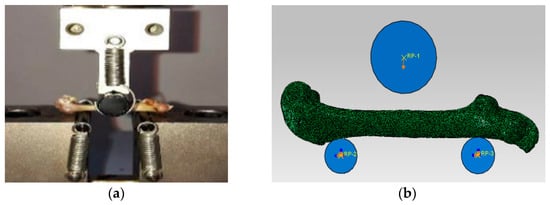
Figure 1.
The schematic diagrams of the experiment on the rat femur and the simulation on the FE model: (a) Three-point bending experiment. (b) Three-point bending simulation.
2.2. Establishment of the Femoral Finite Element Model
Four groups of femoral micro images were respectively imported into the MIMICS software to reconstruct four geometric femoral models, and then the four geometric models were optimized and respectively imported into the ABAQUS software to establish four femoral finite element (FE) models using the C3D8 element, as shown in Figure 1b [17]. Since the apparent fracture of the rat femur under three-point bending load occurred in the middle cortical bone region, as shown in Figure 2, the fracture simulation object in this study is the cortical bone structure. To simulate the experimental boundary conditions, rigid columns were established above and below the femur model, where the relative positions between the three rigid columns and the femur were consistent with the experiment. The interaction between the upper rigid column and the femur was set to frictionless contact, and the interaction between the lower rigid column and the femur was set to TIE contact [18]. The compressive displacement load was applied to the upper rigid column while constraining all the degrees of freedom of the lower rigid columns to achieve the bending condition. Because the static FE analysis was conducted in this simulation, the compressive displacement was the static load, and the maximum displacement load was set to 1 mm. The schematic diagram of the boundary condition in the simulation can be seen in Figure 1b.
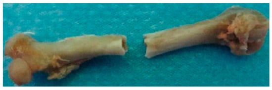
Figure 2.
The schematic diagrams of the apparent fracture of the rat femur under three-point bending load.
The elastic moduli of the cortical bone tissue in the three-month-old Wistar rat femur have been measured by our previous nanoindentation test, where the average value of the transverse elastic modulus is 8769 MPa and the longitudinal elastic modulus is 10,383 MPa [19]. The Poisson’s ratio was set to 0.3 according to the literature [20]. Meanwhile, the critical failure strain and critical energy release rate in the three-month-old Wistar rat femoral cortical bone material had also been obtained from previous studies, where the critical failure strain in compression was 4.35%, in tension was 2.61%, and the critical energy release rate was 0.16 N/mm [10,21,22]. Therefore, all the material input parameters required to perform the fracture simulation using the three numerical methods were known.
2.3. Fracture Simulation Based on the EIF Method
The fracture simulation based on the EIF method is implemented by the subroutine USDFLD in the ABAQUS software. First, a special variable associated with the element stiffness is set up in the subroutine, and the initial value of the special variable is set to 0. At the initial loading, both the maximum and minimum principal strains in the element are low, and the damage initiation has not occurred. Therefore, the value of the special variable is not changed. Then, when the maximum or minimum principal strain in the element reaches the critical tensile or compressive failure strain of the cortical bone material with bending load, the element damage initiates, and the special variable will change to 1. Because the special variable is associated with the element stiffness, the stiffness in the element will drop to zero, and the element will enter the failure stage and loss carrying capacity [9,10]. Finally, as the bending load continues to increase, an apparent fracture will occur in the cortical bone structure when the failed elements reach a certain percentage.
2.4. Fracture Simulation Based on the CDM Method
The fracture simulation based on the CDM method is implemented by the subroutine UMAT in the ABAQUS software. A damage variable is first set up in the program. The stress–strain relationship based on the damage variable for cortical bone structure under quasi-static loading can be expressed as Equations (1) and (2) [23]. When the principal strain in the element reaches the critical failure strain of the cortical bone material, the element will enter the damage initiation stage, and the damage variable will increase with Equation (3) [24]. The element may enter the failure stage as the damage variable reaches to nearly 1. When the failed elements accumulate to a certain level, the cortical bone structure could no longer effectively carry, resulting in an apparent fracture.
where σ is the stress tensor in the element of the finite element model, is the damage elasticity matrix tensor in the element of the finite element model, ε is the strain tensor in the element of the finite element model, D is the damage variable in the element of the finite element model, C is the elasticity matrix tensor in the element of the finite element model, ε is the maximum or minimum principle strain in the element of the finite element model, and εf is the critical tensile or compressive failure strain in the cortical bone material.
2.5. Fracture Simulation Based on the XFEM
All the elements in the FE model are set to the enriched regions in the fracture simulation based on the XFEM. The subroutine UDMIGINI in the ABAQUS software is initially programmed to determine the element damage initiation in compression or tension [25]. The damage initiation criterion is that the maximum or minimum principal strain in the element reaches the critical tensile or compressive failure strain of cortical bone material. The damage evolution law describes the rate at which the element stiffness is degraded once the corresponding damage initiation criterion is reached. The damage evolution law in the element is based on the traction-separation criterion that is embedded in the ABAQUS software. The available traction-separation model in Abaqus assumes initially linear elastic behavior followed by the initiation and evolution of damage. The elastic behavior is written in terms of an elastic constitutive matrix that relates the nominal stresses to the nominal strains across the crack interface, as shown in Equation (4). With crack propagation, the cohesive stiffness of the damaged element at the crack interface gradually decreases, leading to the reduced traction. When the cohesive stiffness degrades to 0, the traction would thoroughly disappear, which results in the apparent fracture [26].
where is the nominal traction stress vector in the element of the finite element model, consists of three components, represents the normal traction, and represent the shear tractions. is the elasticity matrix tensor in the element of the finite element model. represents the normal strain, and and represent the shear strains.
3. Results
Mesh sensitivity analysis was performed to determine the suitable element size for the femoral FE model. Based on the femoral micro images, different element sizes (20, 30, 40, 50, and 60 μm) were selected to establish the femoral FE models. The fracture simulations for the five FE models were all performed based on the CDM method. The load-displacement curves predicted in the simulations with the five FE models were shown in Figure 3. The shape of the curve was similar when the material input parameters were the same. However, certain differences existed in the fracture load and time. The FE model with coarse element underwent complete fracture early because the damage variable rose faster for the large element size, resulting in a faster decrease in the structural stiffness. The predicted three curves had no obvious differences in the fracture parameters when the element size was in the range of 20–40 μm. Therefore, the element size of the femoral FE models established in this study was set to 30 μm considering the prediction accuracy.
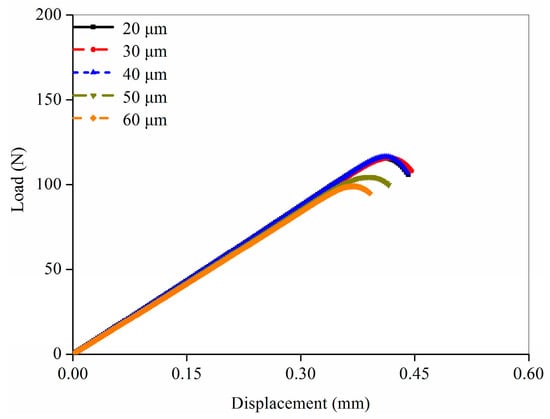
Figure 3.
Mesh sensitivity analysis for the rat femoral FE models with different mesh size.
The load-displacement curves predicted by the three numerical methods expressed different shapes even though the simulated object was the same FE model, as shown in Figure 4. The elastic stage in the curves from the EIF and XFEM simulations nearly coincided, and the apparent stiffness in the elastic stage from the CDM simulation curves gradually decreased. The CDM simulation curves showed a brief yielding phase after the elastic stage, followed by the apparent failure, whereas the EIF and XFEM simulation curves went straight from the elastic stage to the failure stage.
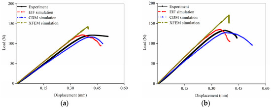
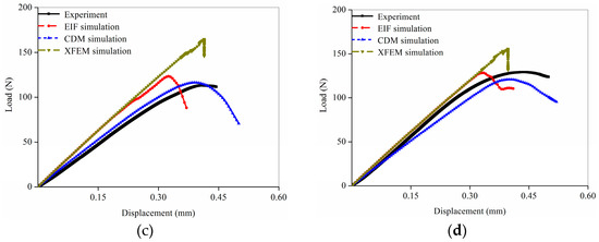
Figure 4.
Comparison of the load-displacement curves obtained from the experiments and three different fracture simulations: (a) Sample 1; (b) Sample 2; (c) Sample 3; (d) Sample 4.
The comparison of the predicted fracture parameters showed different simulation accuracy in the three numerical methods. In the EIF simulation, the apparent failure appeared first compared with other numerical methods; however, the fracture load was not significantly lower than the experimental result because the apparent stiffness in the load-displacement curve was not reduced during the elastic phase. The fracture time obtained from the XFEM simulation was similar to the experimental data, and the fracture load was significantly greater than the experimental results because the apparent stiffness in the curve during the elastic phase was also not reduced. In contrast, the fracture time and fracture load obtained from the CDM simulations were both in better agreement with the experimental results.
Figure 5 shows the comparison of the fracture pattern in the FE model and femur sample under various numerical simulations and experiments. Figure 5a shows the fracture pattern in the EFI simulation. The main crack primarily appeared on the upper side of the middle femur and gradually propagated from the upper to lower sides until it penetrated the outer section of the cortical bone structure, finally leading to the apparent failure. The fracture patterns in the XFEM and CDM simulations were similar, but differed with the EFI simulation, as shown in Figure 5b,c. A few damaged elements first appeared in the upper side of the middle femur close to the rigid column, and then the majority of damaged elements appeared in the lower side of the middle femur with bending load. In the late stage of the loading, the failed elements and the main crack gradually propagated from the lower to upper sides of the middle femur until they penetrated the cortical bone section. This fracture pattern was more similar to the experimental fracture pattern, as shown in Figure 5d. The differences between the fracture patterns predicted by the XFEM and CDM simulations lay in the number of damaged elements. In the CDM simulation, damage occurred as soon as the condition was satisfied, so a certain number of green damaged elements appeared in the constrained and loaded regions. In the XFEM simulation, the entire femoral FE model was set as an enrich region, and the damaged element only appeared in the region where the damage initiation criteria was initially satisfied. Thus, a small number of damaged elements initially appeared on the upper side of the middle femur. However, as these damaged elements could not satisfy the failure condition, many damaged elements reappeared on the lower side of the middle femur. The apparent failure was eventually caused by these damaged elements progressively propagating into failed elements under bending load.
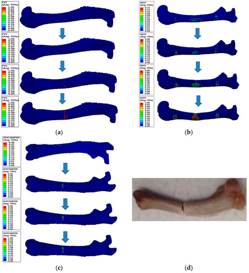
Figure 5.
Comparison of the fracture patterns predicted in the three numerical method simulations and performed in the experiment: (a) fracture simulation based on the EIF method; (b) fracture simulation based on CDM method; (c) fracture simulation based on XFEM; (d) experiment.
4. Discussion
This paper aimed to evaluate the prediction accuracy and applicability of cortical bone fracture in the three different numerical methods. The simulation results predicted by different numerical methods were compared with the experimental data to determine the respective prediction accuracy on the basis of the same material parameters and FE model. The fracture parameters and fracture patterns obtained from the three simulations were compared and analyzed to reveal the cause of the variations in the predicted results and to find a suitable numerical method for simulating cortical bone fracture.
The simulation results showed visible differences in the failure processes, fracture parameters, and fracture patterns predicted by the three simulation methods for the same FE model. First, the cause of the variations in the elastic stage of the load-displacement curves was discussed. The slope of the curve in the elastic stage in the EIF and XFEM simulations was the same and almost did not drop, but the CDM simulation displayed a decreasing trend. This phenomenon was mainly related to the different element failure strategies in the numerical simulation methods. In the EIF simulation, the element included two states, i.e., the elastic and failure states. As the principal strain in the element reached the material failure strain, the element stiffness immediately dropped to 0. The element did not go through the damage evolution process and failure occurred directly. Thus, the apparent stiffness in the elastic stage was not decreased. Though the element would experience the damage initiation and propagation stages in the XFEM simulation, the traction-separation behavior followed by the crack extension is customized in the ABAQUS software to describe the intrinsic matrix of the normal and tangential stresses at the crack interface associated with the normal and tangential separation by elastic relations, resulting in the linear stiffness degradation behavior during the damage evolution stage [26,27]. Thus, the apparent stiffness in the curve was also not decreased in the elastic phase. In the CDM simulation, the element also included the damage initiation and propagation stages. However, the elements follow the nonlinear stiffness degradation criterion during the damage evolution, unlike XFEM. In the elastic phase, a few damaged elements appeared, and the element stiffness gradually decreased with the increasing damage variable, resulting in a slightly dropping trend in the slope of the curve. Because the bending moment was not great at the beginning of the loading, the number of damaged elements was small, and the damaged elements had not yet entered the failure stage and still had the bearing capacity, the dropping trend in the slope was not obvious. The number of the damaged and failed elements gradually increased with bending load, so the slope of the curve in the later elastic stage fell more visibly, which was different from the results obtained by the other two numerical methods. Additionally, Figure 4 demonstrated that the slope displayed a tendency of slowly dropping at the beginning and obviously decreasing at the middle and end of loading in the experimental load-displacement curves. This phenomenon indicated that despite the mechanical behavior in the cortical bone structure and general lack of a visible yielding phase, the osteon in cortical bone may nevertheless exhibit plastic mechanical properties, which is why the quasi-brittle fracture occurred in the cortical bone structure under three-point bending load [28,29].
Second, the causes of the variations in fracture time predicted by the three numerical methods were discussed. The fracture time in the XFEM and CDM simulations was consistent with the experimental results, but in the EIF simulation was earlier than the experimental fracture time. This phenomenon was mainly caused by the element in the EIF simulation lacking a damage evolution process, namely the stiffness changed instantly from its initial value to zero when it reached the damage initiation criterion. In actuality, the osteon still has a certain load-bearing capacity even damage occurs in cortical bone structure [30]. The EIF method directly specified the damage element as failure, which weakened the structural load-bearing capacity and caused the apparent failure to occur earlier than expected. Meanwhile, the causes of the variations in the fracture load predicted by the three numerical methods were also discussed. The fracture load predicted by the EIF and CDM simulations was comparable to the experimental results but considerably less than the value in the XFEM simulation. This phenomenon was caused by the fact that the slope of the load-displacement curve in the XFEM simulation was not dropped before the apparent failure occurred. The predicted fracture load in EIF simulation should express an excessive value because the slope of the curve in the elastic stage was also not decreased; however, the fracture load was lower than the experimental result. This phenomenon was caused by the fact that the load-bearing ability in the cortical bone structure was weakened due to the absence of damage evolution stage in the element in the EIF simulation process, which led to the premature occurrence of the apparent failure.
The differences in the fracture patterns predicted by the three numerical methods can be seen in Figure 5. The reason for the differences in the fracture patterns was mainly related to the various criteria in the element damage and failure processes. The principal strain was high near the indenter at the initial loading, so all three simulations demonstrated that a limited number of damaged elements appeared in the upper side of the middle femur near the indenter. Because the damaged element lost its load-bearing capacity in the EIF simulation, the complete elements near the failed elements must bear more load, which could cause these complete elements to go into failure state quickly due to overload. Therefore, the crack propagated from the upper to lower sides of the middle femur in the EIF simulation. In the CDM and XFEM simulations, at the beginning of loading, the damaged elements in the upper side of the middle femur did not fail and still retained carrying capacity, so the complete elements close to the damaged elements were not overloaded and did not fail. In the middle of loading, the bending moment was transferred from the constraint location to the lower side of the middle femur, and the bending was sufficient to lead to failure in the damaged elements. Therefore, the crack propagated from the lower to upper sides of the middle femur. Furthermore, it has been reported that the femur fracture under three-point bending load is mainly because the continuous propagation of the lower surface crack in the transverse and longitudinal directions cut off the central section of the femoral shaft, which is consistent with the failure processes in the CDM and XFEM simulations [31,32].
The above discussion concluded that the EIF numerical method was more suitable for simulating the brittle fracture because the damage evolution process in the element was not set up and the apparent stiffness was not decreased in the load-displacement curve. Though the damage evolution process was set in the XFEM simulation, the available traction-separation model in the ABAQUS assumes the linear stiffness degradation behavior during the damage evolution in the element, so the apparent stiffness was also not decreased in the elastic stage, which caused the excessive fracture load. Therefore, the XFEM simulation may also be more suitable for simulating the brittle fracture. By contrast, the failure process in the femur under three-point bending was accurately simulated using the CDM method because the slight yielding phase can be predicted. Therefore, the predicted load-displacement curves and fracture patterns in the CDM simulation were consistent with the experimental results.
This paper has several drawbacks in terms of performing the experiment and fracture simulation. First, the loading condition was single because only the three-point bending load was considered. The femur may experience compression, torsion, and impact loads in real life. Second, the three numerical methods were not considered the time-related mechanical properties, resulting in the inability to observe the relationship between the fracture parameters and the loading time. Third, only four femur samples were used to conduct the three-point bending experiment and fracture simulation, which cannot perform the data statistics for the experimental and simulated results. Although the above limitations exist, the main purpose of this study was to investigate the prediction accuracy in the different numerical methods. The numerical method that was suitable for simulating cortical bone fracture under bending load had been determined, and the reason for the differences in the results among the three numerical methods had also been discussed, which assisted in improving the prediction accuracy in cortical bone fracture simulation.
5. Conclusions
Fracture simulations based on the three numerical methods were performed on the same femoral FE model. The fracture simulation based on the CDM method was more consistent with the experimental results. The results showed obvious differences in the fracture parameters and patterns among different simulations. The reason may relate to the different element failure strategies. The elements directly entered the failure state from the elastic state, and the yielding phase could not be reflected in the EIF simulation, so the predicted results were not consistent with the experimental data. The available traction-separation model that is currently supported by ABAQUS assumes the linear stiffness degradation behavior during the damage evolution in the element in the XFEM simulation; consequently, the apparent stiffness was not decreased in the elastic stage, which resulted in an excessive fracture load.
Author Contributions
R.F. implemented the material model in the finite element code and simulated the failure process. J.L. and Z.J. developed models, assisted in data analysis, and generated figures for the manuscript. All authors contributed to this manuscript and approved the submitted version. All authors have read and agreed to the published version of the manuscript.
Funding
The research was funded by the Natural Science Foundation of Jilin Province (YDZJ202301ZYTS250).
Institutional Review Board Statement
This study was approved by the Medical Ethics Committee of the First Hospital of Jilin University (No. 2018-238). This study was in strict accordance with the requirement of the Laboratory Animal Standardization Committee.
Informed Consent Statement
Informed consent was obtained from all subjects involved in the study.
Data Availability Statement
The data used to support the findings of this study are available from the corresponding author upon request.
Conflicts of Interest
The authors declare no conflict of interest.
References
- Li, J.; Gong, H. Fatigue behavior of cortical bone: A review. Acta Mech. Sin. 2020, 37, 516–526. [Google Scholar] [CrossRef]
- Bala, Y.; Zebaze, R.; Seeman, E. Role of cortical bone in bone fragility. Curr. Opin. Rheumatol. 2015, 27, 406–413. [Google Scholar] [CrossRef] [PubMed]
- Sharma, N.K.; Sharma, S.; Rathi, A.; Kumar, A.; Saini, K.V.; Sarker, M.D.; Naghieh, S.; Ning, L.; Chen, D.X. Micromechanisms of Cortical Bone Failure Under Different Loading Conditions. J. Biomech. Eng. 2020, 142, 8. [Google Scholar] [CrossRef] [PubMed]
- Zimmermann, E.A.; Launey, M.E.; Barth, H.D.; Ritchie, R.O. Mixed-mode fracture of human cortical bone. Biomaterials. 2009, 30, 5877–5884. [Google Scholar] [CrossRef]
- Chappard, D.; Baslé, M.; Legrand, E.; Audran, M. New laboratory tools in the assessment of bone quality. Osteoporos. Int. 2011, 22, 2225–2240. [Google Scholar] [CrossRef] [PubMed]
- An, B.; Liu, Y.; Arola, D.; Zhang, D. Fracture toughening mechanism of cortical bone: An experimental and numerical approach. J. Mech. Behav. Biomed. Mater. 2011, 4, 983–992. [Google Scholar] [CrossRef]
- Ural, A.; Vashishth, D. Cohesive finite element modeling of age-related toughness loss in human cortical bone. J. Biomech. 2006, 39, 2974–2982. [Google Scholar] [CrossRef]
- Ural, A.; Bruno, P.; Zhou, B.; Shi, X.T.; Guo, X.E. A new fracture assessment approach coupling HR-pQCT imaging and fracture mechanics-based finite element modeling. J. Biomech. 2013, 46, 1305–1311. [Google Scholar] [CrossRef]
- MacNeil, J.A.; Boyd, S.K. Bone strength at the distal radius can be estimated from high-resolution peripheral quantitative computed tomography and the finite element method. Bone 2008, 42, 1203–1213. [Google Scholar] [CrossRef]
- Fan, R.; Gong, H.; Zhang, R.; Gao, J.; Jia, Z.; Hu, Y. Quantification of Age-Related Tissue-Level Failure Strains of Rat Femoral Cortical Bones Using an Approach Combining Macrocompressive Test and Microfinite Element Analysis. J. Biomech. Eng. 2016, 138, 041006. [Google Scholar] [CrossRef]
- Hambli, R.; Bettamer, A.; Allaoui, S. Finite element prediction of proximal femur fracture pattern based on orthotropic behavior law coupled to quasi-brittle damage. Med. Eng. Phys. 2012, 34, 202–210. [Google Scholar] [CrossRef] [PubMed]
- Kraiem, T.; Barkaoui, A.; Merzouki, T.; Chafra, M. Computational approach of the cortical bone mechanical behavior based on an elastic viscoplastic damageable constitutive model. Int. J. Appl. Mech. 2020, 12, 2050081. [Google Scholar] [CrossRef]
- Salem, M.; Westover, L.; Adeeb, S.; Duke, K. Prediction of fracture initiation and propagation in pelvic bones. Comput. Methods Biomech. Biomed. Eng. 2021, 25, 808–820. [Google Scholar] [CrossRef]
- Feerick, E.M.; Liu, X.; McGarry, P. Anisotropic mode-dependent damage of cortical bone using the extended finite element method (XFEM). J. Mech. Behav. Biomed. Mater. 2013, 20, 77–89. [Google Scholar] [CrossRef] [PubMed]
- Kumar, A.; Ghosh, R. A review on experimental and numerical investigations of cortical bone fracture. Proc. Inst. Mech. Eng. Part H J. Eng. Med. 2022, 236, 297–319. [Google Scholar] [CrossRef] [PubMed]
- Fang, J.; Gao, J.; Gong, H.; Zhang, T.; Zhang, R.; Zhan, B. Multiscale experimental study on the effects of different weight-bearing levels during moderate treadmill exercise on bone quality in growing female rats. Biomed. Eng. Online 2019, 18, 33. [Google Scholar] [CrossRef]
- Fan, R.X.; Liu, J.; Liu, J. Prediction of the natural frequencies of different degrees of degenerated human lumbar segments L2-L3 using dynamic finite element analysis. Comput. Methods Programs Biomed. 2022, 209, 106352. [Google Scholar] [CrossRef]
- Ridha, H.; Thurner, P.J. Finite element prediction with experimental validation of damage distribution in single trabeculae during three-point bending tests. J. Mech. Behav. Biomed. Mater. 2013, 27, 94–106. [Google Scholar] [CrossRef]
- Zhang, R.; Gong, H.; Zhu, D.; Ma, R.; Fang, J.; Fan, Y. Multi-level femoral morphology and mechanical properties of rats of different ages. Bone. 2015, 76, 76–87. [Google Scholar] [CrossRef]
- Osuna, L.G.G.; Soares, C.J.; Vilela, A.B.F.; Irie, M.S.; Versluis, A.; Soares, P.B.F. Influence of bone defect position and span in 3-point bending tests: Experimental and finite element analysis. Braz. Oral Res. 2021, 35, e001. [Google Scholar] [CrossRef]
- Kumar, A.; Shitole, P.; Ghosh, R.; Kumar, R.; Gupta, A. Experimental and numerical comparisons between finite element method, element-free Galerkin method, and extended finite element method predicted stress intensity factor and energy release rate of cortical bone considering anisotropic bone modelling. Proc. Inst. Mech. Eng. Part H: J. Eng. Med. 2019, 233, 823–838. [Google Scholar] [CrossRef] [PubMed]
- Giner, E.; Belda, R.; Arango, C.; Vercher-Martínez, A.; Tarancón, J.E.; Fuenmayor, F.J. Calculation of the critical energy release rate Gc of the cement line in cortical bone combining experimental tests and finite element models. Eng. Fract. Mech. 2017, 184, 168–182. [Google Scholar] [CrossRef]
- Hambli, R.; Allaoui, S. A Robust 3D Finite Element Simulation of Human Proximal Femur Progressive Fracture Under Stance Load with Experimental Validation. Ann. Biomed. Eng. 2013, 41, 2515–2527. [Google Scholar] [CrossRef] [PubMed]
- Gaziano, P.; Falcinelli, C.; Vairo, G. A computational insight on damage-based constitutive modelling in femur mechanics. Eur. J. Mech. A/Solids 2022, 93, 104538. [Google Scholar] [CrossRef]
- Fan, R.; Gong, H.; Zhang, X.; Liu, J.; Jia, Z.; Zhu, D. Modeling the Mechanical Consequences of Age-Related Trabecular Bone Loss by XFEM Simulation. Comput. Math. Methods Med. 2016, 2016, 3495152. [Google Scholar] [CrossRef]
- Gustafsson, A.; Wallin, M.; Khayyeri, H.; Isaksson, H. Crack propagation in cortical bone is affected by the characteristics of the cement line: A parameter study using an XFEM interface damage model. Biomech. Model. Mechanobiol. 2019, 18, 1247–1261. [Google Scholar] [CrossRef]
- Salem, M.; Westover, L.M.; Adeeb, S.M.; Duke, K. An Equivalent Constitutive Model of Cancellous Bone With Fracture Prediction. J. Biomech. Eng. 2020, 142, 121004. [Google Scholar] [CrossRef]
- Ng, T.P.; Koloor, S.S.R.; Djuansjah, J.R.P.; Kadir, M.A. Assessment of compressive failure process of cortical bone materials using damage-based model. J. Mech. Behav. Biomed. Mater. 2017, 66, 1–11. [Google Scholar] [CrossRef]
- Hambli, R. A quasi-brittle continuum damage finite element model of the human proximal femur based on element deletion. Med. Biol. Eng. Comput. 2012, 51, 219–231. [Google Scholar] [CrossRef]
- Yadav, R.N.; Uniyal, P.; Sihota, P.; Kumar, S.; Dhiman, V.; Goni, V.G.; Sahni, D.; Bhadada, S.K.; Kumar, N. Effect of ageing on microstructure and fracture behavior of cortical bone as determined by experiment and Extended Finite Element Method (XFEM). Med. Eng. Phys. 2021, 93, 100–112. [Google Scholar] [CrossRef]
- Khor, F.; Cronin, D.; Watson, B.; Gierczycka, D.; Malcolm, S. Importance of asymmetry and anisotropy in predicting cortical bone response and fracture using human body model femur in three-point bending and axial rotation. J. Mech. Behav. Biomed. Mater. 2018, 87, 213–229. [Google Scholar] [CrossRef] [PubMed]
- Laurent, C.; Bohme, B.; Mengoni, M.; Otreppe, V.; Balligand, M.; Ponthot, J.P. Prediction of the mechanical response of canine humerus to three-point bending using subject-specific finite element modelling. Proc. Inst. Mech. Eng. H 2016, 230, 639–649. [Google Scholar] [CrossRef] [PubMed]
Disclaimer/Publisher’s Note: The statements, opinions and data contained in all publications are solely those of the individual author(s) and contributor(s) and not of MDPI and/or the editor(s). MDPI and/or the editor(s) disclaim responsibility for any injury to people or property resulting from any ideas, methods, instructions or products referred to in the content. |
© 2023 by the authors. Licensee MDPI, Basel, Switzerland. This article is an open access article distributed under the terms and conditions of the Creative Commons Attribution (CC BY) license (https://creativecommons.org/licenses/by/4.0/).