

Implicit Bias of Deep Learning in the Large Learning Rate Phase: A Data Separability Perspective

Abstract
1. Introduction
- According to the separation conditions of the data, we characterize the dynamics of gradient descent with logistic and exponential loss corresponding to the learning rate. We find that the gradient descent iterates converge to a flatter minimum in the catapult phase when the data is non-separable. The above three learning rate phases do not apply to the linearly separable data since the optimum is towards infinity.
- Our theoretical analysis ranges from a linear predictor to a one-hidden-layer network. By comparing the convex optimization characterized by Theorem 1 and non-convex optimization characterized by Theorem A2 in terms of the learning rate, we show that the catapult phase is a unique phenomenon for non-convex optimizations.
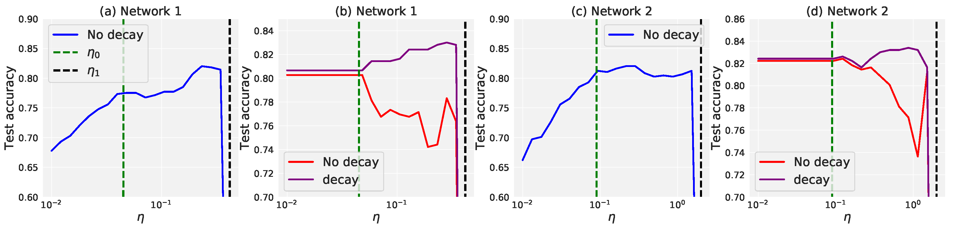
- We find that in practical classification tasks, the best generalization results tend to occur in the catapult phase. Given the fact that the infinite-width analysis (lazy training) does not fully explain the empirical power of deep learning, our results can be used to partially fill this gap.
2. Related Work
2.1. Implicit Bias of Gradient Methods
2.2. Data Separability
2.3. Neural Tangent Kernel
2.4. Large Learning Rate and Logistic Loss
3. Background
3.1. Setup
3.2. Separation Conditions of Dataset
- 1
- Under Assumption 1, the empirical loss is β-smooth. Then the gradient descent with constant learning rate never increases the risk, and empirical loss will converge to zero:
- 2
- Under Assumption 2, the empirical loss is β-smooth and α-strongly convex, where . Then the gradient descent with a constant learning rate never increases the risk, and empirical loss will converge to a global minimum. On the other hand, the gradient descent with a constant learning rate never decreases the risk, and empirical loss will explode or saturate:where is the value of a global minimum while for exploding situation or when saturating.
4. Theoretical Results
4.1. Convex Optimization
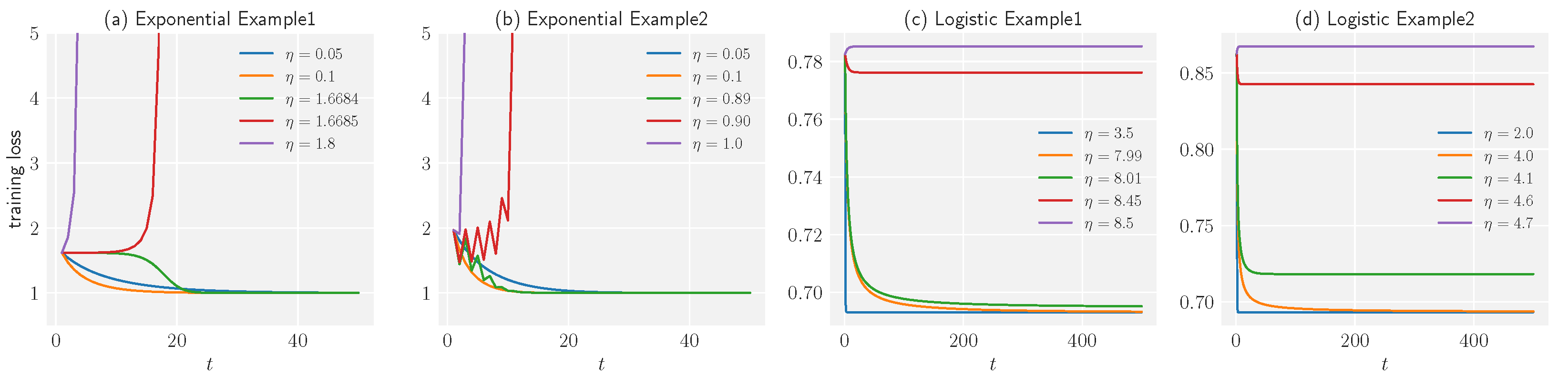
- 1
- For exponential loss, the gradient descent with a constant learning rate never increases loss, and the empirical loss converges to the global minimum. On the other hand, the gradient descent with learning rate oscillates. Finally, when the learning rate , the training process never decreases the loss and the empirical loss will explode to infinity:
- 2
- For logistic loss, the critical learning rate satisfies the condition: . The gradient descent with a constant learning rate never increases the loss, and the loss converges to the global minimum. On the other hand, the loss along with a learning rate does not converge to the global minimum but oscillates. Finally, when the learning rate , gradient descent never decreases the loss, and the loss saturates:where satisfies .
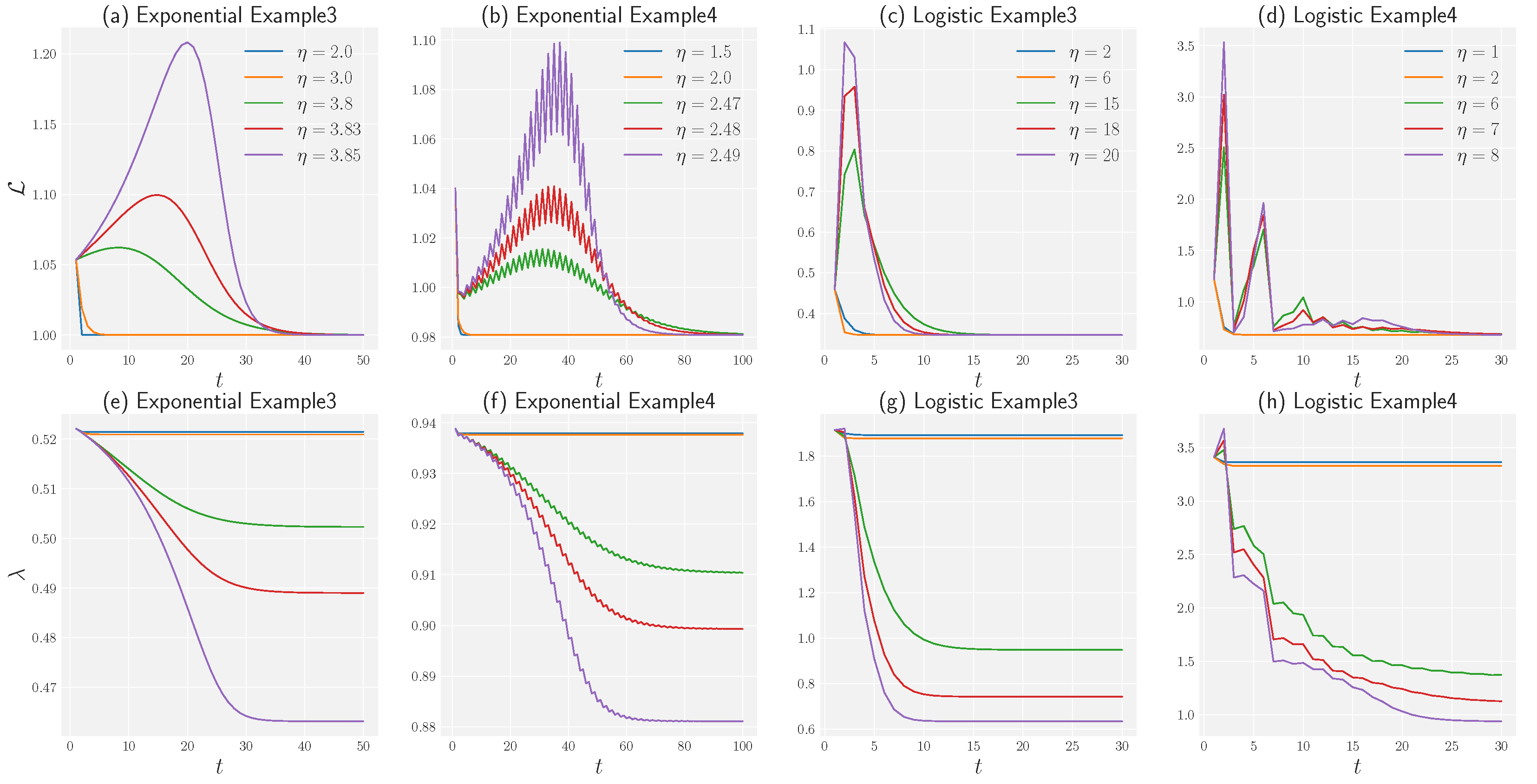
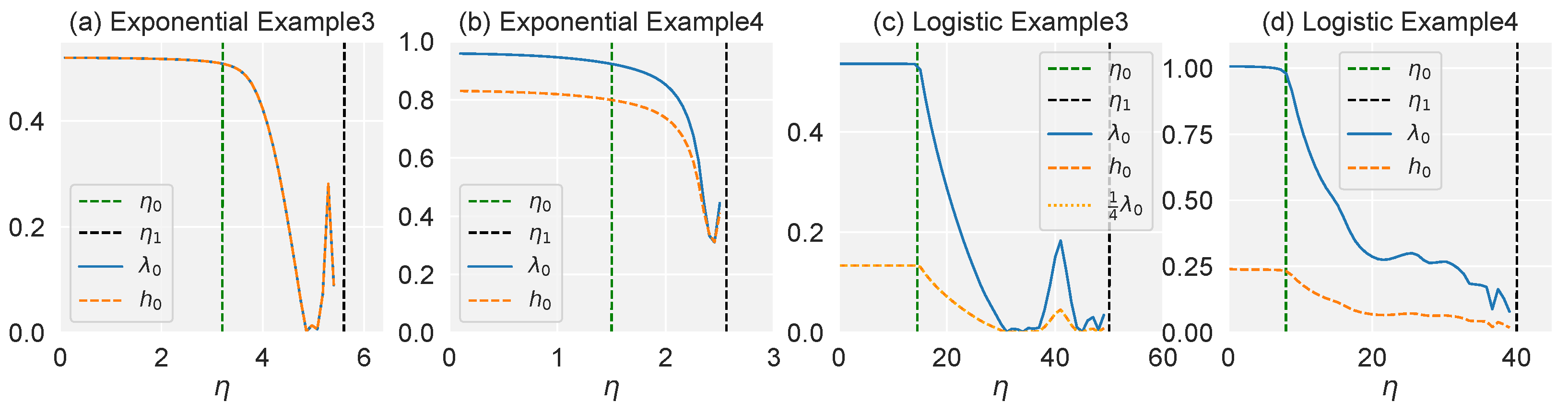
4.2. Non-Convex Optimization
- 1.
- keeps increasing when .
- 2.
- After the T step and its successors, the loss decreases, which is equivalent to:
- 3.
- The eigenvalue of NTK keeps dropping after the T steps:
5. Experiment
5.1. Experimental Results
5.2. Effectiveness on Synthetic and Real-World Datasets
6. Discussion
Author Contributions
Funding
Institutional Review Board Statement
Informed Consent Statement
Data Availability Statement
Conflicts of Interest
Appendix A
- 1
- Under Assumption 1, the empirical loss is β-smooth. Then the gradient descent with constant learning rate never increases the risk, and empirical loss will converge to zero:
- 2
- Under Assumption 2, the empirical loss is β-smooth and α-strongly convex, where . Then the gradient descent with a constant learning rate never increases the risk, and empirical loss will converge to a global minimum. On the other hand, the gradient descent with a constant learning rate never decreases the risk, and empirical loss will explode or saturate:where is the value of a global minimum while for exploding situation or when saturating.
- 1
- We first prove that empirical loss regrading data-scaled weight for the linearly separable dataset is smooth. The empirical loss can be written as , then the second derivatives of logistic and exponential loss are,when is limited, there will be a such that . Furthermore, because there exists a separator such that , the second derivative of empirical loss can be arbitrarily close to zero. This implies that the empirical loss function is not strongly convex.Recalling a property of the -smooth function f [60],Taking the gradient descent into consideration,when , that is , we have,We now prove that empirical loss will converge to zero with learning rate . We changing the form of the above inequality,this implies,therefore, we have .
- 2
- When the data is not linear separable, there is no such that . Thus, at least one is negative when the other terms are positive. This implies that the solution of the loss function is finite and the empirical loss is both -strongly convex and -smooth.Taking the gradient descent into consideration,when , that is , we have,
- 1
- For exponential loss, the gradient descent with a constant learning rate never increases loss, and the empirical loss will converge to the global minimum. On the other hand, the gradient descent with learning rate will oscillate. Finally, when the learning rate , the training process never decreases the loss and the empirical loss will explode to infinity:
- 2
- For logistic loss, the critical learning rate satisfies a condition: . The gradient descent with a constant learning rate never increases the loss, and the loss will converge to the global minimum. On the other hand, the loss along with a learning rate will not converge to the global minimum but oscillate. Finally, when the learning rate , gradient descent never decreases the loss, and the loss will saturate:where satisfies .
- 1
- Under the degeneracy assumption, the risk is given by the hyperbolic function . The update function for the single weight is,To compare the norm of the gradient and the norm of loss, we introduce the following function:Then it is easy to see thatIn this way, we have transformed the problem into studying the iso-surface of . Define byLet be the complementary set of in . Since is monotonically increasing, we know that is connected and contains .Suppose , then , which implies thatThus, the first step becomes trapped in :By induction, we can prove that for arbitrary , which is equivalent toSimilarly, we can prove the theorem under another toe initial conditions: and .
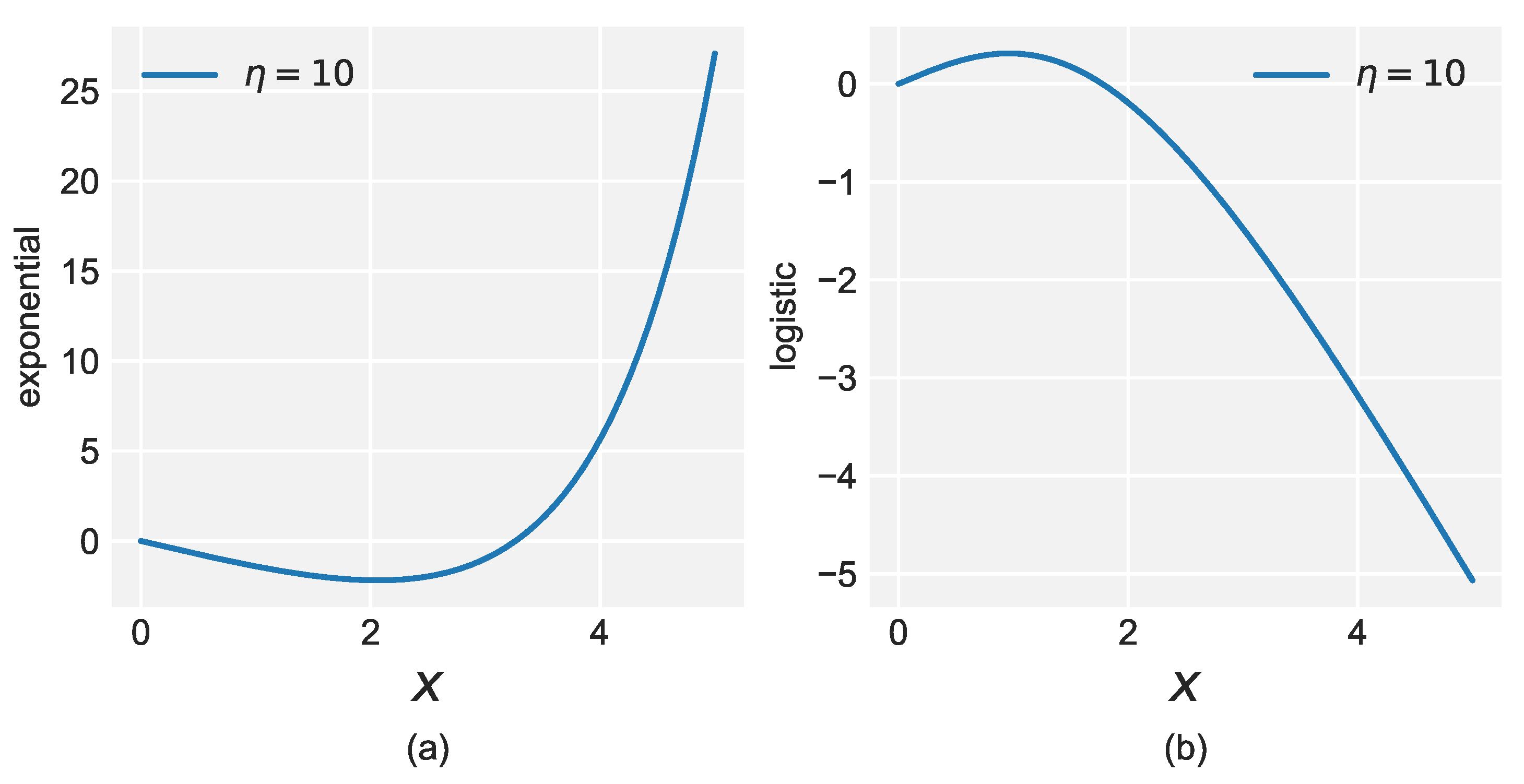
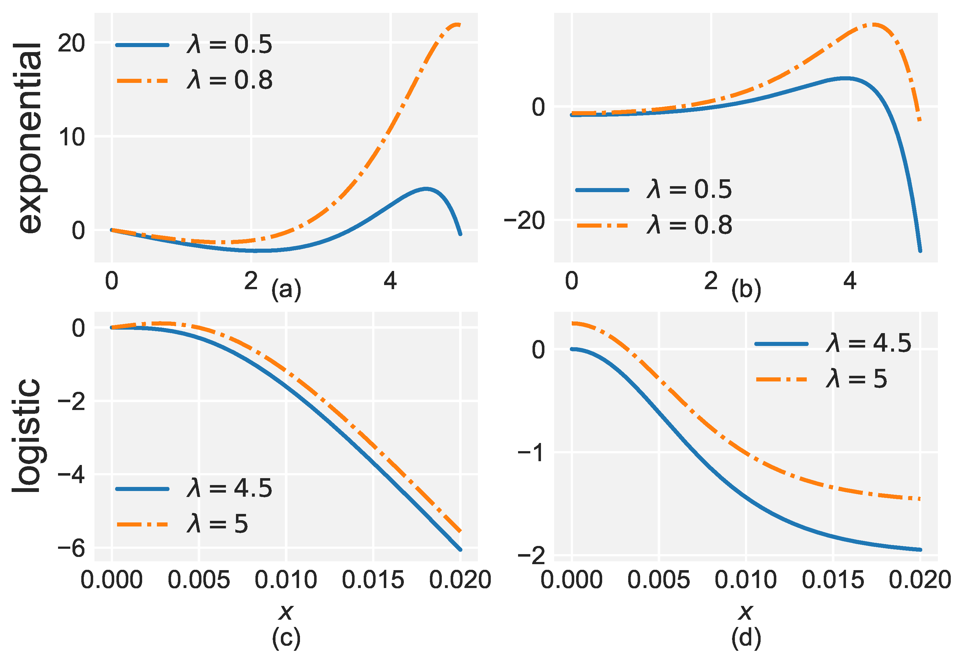
- 2
- Under the degeneracy assumption, the risk is governed by the hyperbolic function . The update function for the single weight is,Thus,Unlike the exponential loss, is monotonically decreasing, which means that of does not contain (see Figure A1).Figure A1. Graph of for the two losses. (a) Exponential loss with learning rate . (b) Logistic loss with learning rate .Figure A1. Graph of for the two losses. (a) Exponential loss with learning rate . (b) Logistic loss with learning rate .
 Suppose , then lies in . In this situation, we denote the critical point that separates and by . That isThen it is obvious that before arrives at , it keeps decreasing and will eventually become trapped at :and we have When , is empty. In this case, we can prove by induction that for arbitrary , which is equivalent to

- 1.
- keeps increasing when .
- 2.
- After the T step and its successors, the loss decreases, which is equivalent to:
- 3.
- The eigenvalue of NTK keeps dropping after the T steps:
- .
- has exponential growth as .
- , this implies thatFor the step and its successors,
- The norm of the NTK keeps dropping after T steps:

- .
References
- Jacot, A.; Gabriel, F.; Hongler, C. Neural tangent kernel: Convergence and generalization in neural networks. In Proceedings of the Advances in Neural Information Processing Systems, Red Hook, NY, USA, 3–8 December 2018; pp. 8571–8580. [Google Scholar]
- Allen-Zhu, Z.; Li, Y.; Song, Z. A convergence theory for deep learning via over-parameterization. In Proceedings of the International Conference on Machine Learning. PMLR, Long Beach, CA, USA, 9–15 June 2019; pp. 242–252. [Google Scholar]
- Du, S.S.; Lee, J.D.; Li, H.; Wang, L.; Zhai, X. Gradient descent finds global minima of deep neural networks. arXiv 2018, arXiv:1811.03804. [Google Scholar]
- Chizat, L.; Bach, F. On the global convergence of gradient descent for over-parameterized models using optimal transport. In Proceedings of the Advances in Neural Information Processing Systems, Red Hook, NY, USA, 3–8 December 2018; pp. 3036–3046. [Google Scholar]
- Zou, D.; Cao, Y.; Zhou, D.; Gu, Q. Stochastic gradient descent optimizes over-parameterized deep ReLU networks. arXiv 2018, arXiv:1811.08888. [Google Scholar]
- Huang, W.; Liu, C.; Chen, Y.; Liu, T.; Da Xu, R.Y. Demystify Optimization and Generalization of Over-parameterized PAC-Bayesian Learning. arXiv 2022, arXiv:2202.01958. [Google Scholar]
- Nakkiran, P.; Kaplun, G.; Bansal, Y.; Yang, T.; Barak, B.; Sutskever, I. Deep double descent: Where bigger models and more data hurt. arXiv 2019, arXiv:1912.02292. [Google Scholar] [CrossRef]
- Soudry, D.; Hoffer, E.; Nacson, M.S.; Gunasekar, S.; Srebro, N. The implicit bias of gradient descent on separable data. J. Mach. Learn. Res. 2018, 19, 2822–2878. [Google Scholar]
- Neyshabur, B.; Tomioka, R.; Srebro, N. In search of the real inductive bias: On the role of implicit regularization in deep learning. arXiv 2014, arXiv:1412.6614. [Google Scholar]
- Gunasekar, S.; Lee, J.; Soudry, D.; Srebro, N. Characterizing implicit bias in terms of optimization geometry. arXiv 2018, arXiv:1802.08246. [Google Scholar]
- Ji, Z.; Telgarsky, M. The implicit bias of gradient descent on nonseparable data. In Proceedings of the Conference on Learning Theory, Phoenix, AZ, USA, 25–28 June 2019; pp. 1772–1798. [Google Scholar]
- Nacson, M.S.; Gunasekar, S.; Lee, J.D.; Srebro, N.; Soudry, D. Lexicographic and depth-sensitive margins in homogeneous and non-homogeneous deep models. arXiv 2019, arXiv:1905.07325. [Google Scholar]
- Lyu, K.; Li, J. Gradient descent maximizes the margin of homogeneous neural networks. arXiv 2019, arXiv:1906.05890. [Google Scholar]
- He, K.; Zhang, X.; Ren, S.; Sun, J. Deep residual learning for image recognition. In Proceedings of the IEEE Conference on Computer Vision and Pattern Recognition, Las Vegas, NV, USA, 26 June–1 July 2016; pp. 770–778. [Google Scholar]
- Zagoruyko, S.; Komodakis, N. Wide residual networks. arXiv 2016, arXiv:1605.07146. [Google Scholar]
- Lewkowycz, A.; Bahri, Y.; Dyer, E.; Sohl-Dickstein, J.; Gur-Ari, G. The large learning rate phase of deep learning: The catapult mechanism. arXiv 2020, arXiv:2003.02218. [Google Scholar]
- Arora, S.; Du, S.S.; Hu, W.; Li, Z.; Salakhutdinov, R.R.; Wang, R. On exact computation with an infinitely wide neural net. In Proceedings of the Advances in Neural Information Processing Systems, Vancouver, BC, Canada, 8–14 December 2019; pp. 8141–8150. [Google Scholar]
- Yang, G. Scaling limits of wide neural networks with weight sharing: Gaussian process behavior, gradient independence, and neural tangent kernel derivation. arXiv 2019, arXiv:1902.04760. [Google Scholar]
- Huang, J.; Yau, H.T. Dynamics of deep neural networks and neural tangent hierarchy. arXiv 2019, arXiv:1909.08156. [Google Scholar]
- Allen-Zhu, Z.; Li, Y. What Can ResNet Learn Efficiently, Going Beyond Kernels? In Proceedings of the Advances in Neural Information Processing Systems, Vancouver, BC, Canada, 8–14 December2019; pp. 9017–9028. [Google Scholar]
- Chizat, L.; Oyallon, E.; Bach, F. On lazy training in differentiable programming. In Proceedings of the Advances in Neural Information Processing Systems, Vancouver, BC, Canada, 8–14 December2019; pp. 2937–2947. [Google Scholar]
- Cohen, G.; Afshar, S.; Tapson, J.; Van Schaik, A. EMNIST: Extending MNIST to handwritten letters. In Proceedings of the 2017 international joint conference on neural networks (IJCNN), Anchorage, AK, USA, 14–19 May 2017; pp. 2921–2926. [Google Scholar]
- Ho-Phuoc, T. CIFAR10 to compare visual recognition performance between deep neural networks and humans. arXiv 2018, arXiv:1811.07270. [Google Scholar]
- Jiang, L.; Zhou, Z.; Leung, T.; Li, L.J.; Fei-Fei, L. MentorNet: Learning Data-Driven Curriculum for Very Deep Neural Networks on Corrupted Labels. In Proceedings of the ICML, Stockholm, Sweden, 10–15 July 2018. [Google Scholar]
- Li, W.; Wang, L.; Li, W.; Agustsson, E.; Van Gool, L. Webvision database: Visual learning and understanding from web data. arXiv 2017, arXiv:1708.02862. [Google Scholar]
- Ali, A.; Dobriban, E.; Tibshirani, R.J. The Implicit Regularization of Stochastic Gradient Flow for Least Squares. arXiv 2020, arXiv:2003.07802. [Google Scholar]
- Mousavi-Hosseini, A.; Park, S.; Girotti, M.; Mitliagkas, I.; Erdogdu, M.A. Neural Networks Efficiently Learn Low-Dimensional Representations with SGD. arXiv 2022, arXiv:2209.14863. [Google Scholar]
- Nacson, M.S.; Lee, J.D.; Gunasekar, S.; Savarese, P.H.; Srebro, N.; Soudry, D. Convergence of gradient descent on separable data. arXiv 2018, arXiv:1803.01905. [Google Scholar]
- Gunasekar, S.; Lee, J.D.; Soudry, D.; Srebro, N. Implicit bias of gradient descent on linear convolutional networks. In Proceedings of the Advances in Neural Information Processing Systems, Red Hook, NY, USA, 3–8 December 2018; pp. 9461–9471. [Google Scholar]
- Ji, Z.; Telgarsky, M. Gradient descent aligns the layers of deep linear networks. arXiv 2018, arXiv:1810.02032. [Google Scholar]
- Razin, N.; Cohen, N. Implicit Regularization in Deep Learning May Not Be Explainable by Norms. arXiv 2020, arXiv:2005.06398. [Google Scholar]
- Smith, S.L.; Dherin, B.; Barrett, D.G.; De, S. On the origin of implicit regularization in stochastic gradient descent. arXiv 2021, arXiv:2101.12176. [Google Scholar]
- Ji, Z.; Telgarsky, M. Directional convergence and alignment in deep learning. arXiv 2020, arXiv:2006.06657. [Google Scholar]
- Chizat, L.; Bach, F. Implicit bias of gradient descent for wide two-layer neural networks trained with the logistic loss. arXiv 2020, arXiv:2002.04486. [Google Scholar]
- Oymak, S.; Soltanolkotabi, M. Overparameterized nonlinear learning: Gradient descent takes the shortest path? arXiv 2018, arXiv:1812.10004. [Google Scholar]
- Nguyen, T.; Novak, R.; Xiao, L.; Lee, J. Dataset distillation with infinitely wide convolutional networks. Adv. Neural Inf. Process. Syst. 2021, 34, 5186–5198. [Google Scholar]
- Ho, T.K.; Basu, M. Complexity measures of supervised classification problems. IEEE Trans. Pattern Anal. Mach. Intell. 2002, 24, 289–300. [Google Scholar]
- Lorena, A.C.; Garcia, L.P.; Lehmann, J.; Souto, M.C.; Ho, T.K. How complex is your classification problem? a survey on measuring classification complexity. ACM Comput. Surv. (CSUR) 2019, 52, 1–34. [Google Scholar] [CrossRef]
- Guan, S.; Loew, M.; Ko, H. Data separability for neural network classifiers and the development of a separability index. arXiv 2020, arXiv:2005.13120. [Google Scholar]
- Rostami, M.; Berahmand, K.; Nasiri, E.; Forouzandeh, S. Review of swarm intelligence-based feature selection methods. Eng. Appl. Artif. Intell. 2021, 100, 104210. [Google Scholar] [CrossRef]
- Berahmand, K.; Mohammadi, M.; Saberi-Movahed, F.; Li, Y.; Xu, Y. Graph regularized nonnegative matrix factorization for community detection in attributed networks. IEEE Trans. Netw. Sci. Eng. 2022, 10, 372–385. [Google Scholar] [CrossRef]
- Bietti, A.; Bruna, J.; Sanford, C.; Song, M.J. Learning Single-Index Models with Shallow Neural Networks. arXiv 2022, arXiv:2210.15651. [Google Scholar]
- Lee, J.; Xiao, L.; Schoenholz, S.; Bahri, Y.; Novak, R.; Sohl-Dickstein, J.; Pennington, J. Wide neural networks of any depth evolve as linear models under gradient descent. In Proceedings of the Advances in Neural Information Processing Systems, Vancouver, BC, Canada, 8–14 December 2019; pp. 8570–8581. [Google Scholar]
- Huang, W.; Du, W.; Da Xu, R.Y. On the Neural Tangent Kernel of Deep Networks with Orthogonal Initialization. arXiv 2020, arXiv:2004.05867. [Google Scholar]
- Li, Z.; Wang, R.; Yu, D.; Du, S.S.; Hu, W.; Salakhutdinov, R.; Arora, S. Enhanced convolutional neural tangent kernels. arXiv 2019, arXiv:1911.00809. [Google Scholar]
- Du, S.S.; Hou, K.; Salakhutdinov, R.R.; Poczos, B.; Wang, R.; Xu, K. Graph neural tangent kernel: Fusing graph neural networks with graph kernels. In Proceedings of the Advances in Neural Information Processing Systems, Vancouver, BC, Canada, 8–14 December 2019; pp. 5723–5733. [Google Scholar]
- Huang, W.; Li, Y.; Du, W.; Yin, J.; Da Xu, R.Y.; Chen, L.; Zhang, M. Towards deepening graph neural networks: A GNTK-based optimization perspective. arXiv 2021, arXiv:2103.03113. [Google Scholar]
- Hron, J.; Bahri, Y.; Sohl-Dickstein, J.; Novak, R. Infinite attention: NNGP and NTK for deep attention networks. arXiv 2020, arXiv:2006.10540. [Google Scholar]
- Jacot, A.; Gabriel, F.; Hongler, C. Freeze and chaos for dnns: An NTK view of batch normalization, checkerboard and boundary effects. arXiv 2019, arXiv:1907.05715. [Google Scholar]
- Yang, G. Tensor Programs II: Neural Tangent Kernel for Any Architecture. arXiv 2020, arXiv:2006.14548. [Google Scholar]
- Krizhevsky, A.; Sutskever, I.; Hinton, G.E. Imagenet classification with deep convolutional neural networks. In Proceedings of the Advances in neural information processing systems, Lake Tahoe, NV, USA, 3–6 December 2012; pp. 1097–1105. [Google Scholar]
- Keskar, N.S.; Mudigere, D.; Nocedal, J.; Smelyanskiy, M.; Tang, P.T.P. On large-batch training for deep learning: Generalization gap and sharp minima. arXiv 2016, arXiv:1609.04836. [Google Scholar]
- Jiang, Y.; Neyshabur, B.; Mobahi, H.; Krishnan, D.; Bengio, S. Fantastic generalization measures and where to find them. arXiv 2019, arXiv:1912.02178. [Google Scholar]
- Li, Y.; Wei, C.; Ma, T. Towards explaining the regularization effect of initial large learning rate in training neural networks. In Proceedings of the Advances in Neural Information Processing Systems, Vancouver, BC, Canada, 8–14 December 2019; pp. 11674–11685. [Google Scholar]
- Nitanda, A.; Chinot, G.; Suzuki, T. Gradient Descent can Learn Less Over-parameterized Two-layer Neural Networks on Classification Problems. arXiv 2019, arXiv:1905.09870. [Google Scholar]
- Nilsen, G.K.; Munthe-Kaas, A.Z.; Skaug, H.J.; Brun, M. Efficient computation of hessian matrices in tensorflow. arXiv 2019, arXiv:1905.05559. [Google Scholar]
- Patrini, G.; Rozza, A.; Krishna Menon, A.; Nock, R.; Qu, L. Making deep neural networks robust to label noise: A loss correction approach. In Proceedings of the IEEE Conference on Computer Vision and Pattern Recognition, Honolulu, HI, USA, 21–26 July 2017; pp. 1944–1952. [Google Scholar]
- Ma, X.; Wang, Y.; Houle, M.E.; Zhou, S.; Erfani, S.M.; Xia, S.T.; Wijewickrema, S.; Bailey, J. Dimensionality-Driven Learning with Noisy Labels. In Proceedings of the ICML, Stockholm, Sweden, 10–15 July 2018. [Google Scholar]
- Ma, X.; Huang, H.; Wang, Y.; Romano, S.; Erfani, S.; Bailey, J. Normalized loss functions for deep learning with noisy labels. In Proceedings of the International Conference on Machine Learning, Atlanta, GA, USA, 16–21 June 2013; PMLR: New York, NY, USA, 2020; pp. 6543–6553. [Google Scholar]
- Bubeck, S. Convex optimization: Algorithms and complexity. arXiv 2014, arXiv:1405.4980. [Google Scholar]


| Symbol | Definition |
|---|---|
| x | Input |
| y | Label |
| Learning rate | |
| Loss function | |
| Empirical loss | |
| Parameters of the model at time step t | |
| -smooth convexity | |
| -strongly convexity | |
| Neural Tangent Kernel |
| Separation Condition | Linear Separable | Degenerate | Non-Separable |
|---|---|---|---|
| Exponential loss (this work) | ✗ | ✓ | ✓ |
| Logistic loss (this work) | ✗ | ✓ | ✓ |
| Squared loss ([16]) | ✓ | ✓ | ✓ |
| Datasets | Methods | Clean | Symmetric Noise Rate () | |||
|---|---|---|---|---|---|---|
| 0.1 | 0.2 | 0.3 | 0.4 | |||
| MNIST | SL | |||||
| OS | ||||||
| EXP | ||||||
| CIFAR-10 | SL | |||||
| OS | ||||||
| EXP | ||||||
| CIFAR-100 | SL | |||||
| OS | ||||||
| EXP | ||||||
| Datasets | Methods | Clean | Asymmetric Noise Rate () | |||
|---|---|---|---|---|---|---|
| 0.1 | 0.2 | 0.3 | 0.4 | |||
| MNIST | SL | |||||
| OS | ||||||
| EXP | ||||||
| CIFAR-10 | SL | |||||
| OS | ||||||
| EXP | ||||||
| CIFAR-100 | SL | |||||
| OS | ||||||
| EXP | ||||||
| Loss | SL | OS | EXP |
|---|---|---|---|
| Acc | 60.38 | 66.04 | 65.92 |
Disclaimer/Publisher’s Note: The statements, opinions and data contained in all publications are solely those of the individual author(s) and contributor(s) and not of MDPI and/or the editor(s). MDPI and/or the editor(s) disclaim responsibility for any injury to people or property resulting from any ideas, methods, instructions or products referred to in the content. |
© 2023 by the authors. Licensee MDPI, Basel, Switzerland. This article is an open access article distributed under the terms and conditions of the Creative Commons Attribution (CC BY) license (https://creativecommons.org/licenses/by/4.0/).
Share and Cite
Liu, C.; Huang, W.; Xu, R.Y.D. Implicit Bias of Deep Learning in the Large Learning Rate Phase: A Data Separability Perspective. Appl. Sci. 2023, 13, 3961. https://doi.org/10.3390/app13063961
Liu C, Huang W, Xu RYD. Implicit Bias of Deep Learning in the Large Learning Rate Phase: A Data Separability Perspective. Applied Sciences. 2023; 13(6):3961. https://doi.org/10.3390/app13063961
Chicago/Turabian StyleLiu, Chunrui, Wei Huang, and Richard Yi Da Xu. 2023. "Implicit Bias of Deep Learning in the Large Learning Rate Phase: A Data Separability Perspective" Applied Sciences 13, no. 6: 3961. https://doi.org/10.3390/app13063961
APA StyleLiu, C., Huang, W., & Xu, R. Y. D. (2023). Implicit Bias of Deep Learning in the Large Learning Rate Phase: A Data Separability Perspective. Applied Sciences, 13(6), 3961. https://doi.org/10.3390/app13063961