Abstract
A data-driven indirect approach for predicting the response of existing structures induced by excavation is hereby proposed based on making full use of monitoring data during excavation, which can predict the deformation history of the research object during excavation. In this article, a machine-learning-based model framework for implementing the proposed approach is constructed and the treatment of key issues in the design and implementation of the proposed method is described in detail including the theoretical framework, the implementation mode of the method, the dimensionality reduction of the model parameters, and the normalization of data for model. On this basis, three models are provided to predict the settlement of buildings induced by adjacent excavation, namely the SVM model, BP model, and BP–SVM model. Relying on an excavation project for a subway in Xuzhou, Jiangsu Province, China, the proposed method is verified, and some conclusions are obtained.
1. Introduction
With the ongoing development of urbanization in China, the high-rise and super-high-rise buildings and the infrastructure such as roads, subways, and utility tunnels spring up continuously in major cities, which make the effective space of urban construction smaller and the construction environment more complex. The existing infrastructure and buildings are inevitably affected by adjacent excavation. Therefore, the safety of the surrounding environment during excavation has become a focus of attention, and much fruitful research on the hot issues of underground excavation and its induced site deformation in infrastructure construction has been published [1,2,3,4,5,6,7,8,9,10,11,12,13,14]. Meanwhile, the safety of existing buildings and utilities close to excavation is receiving more and more attention [15,16,17,18,19,20,21,22,23,24,25,26,27,28].
The major methods [12,29] for investigating the response of the surrounding environment induced by adjacent excavation include analytic approaches [14], empirical formulae [30], numerical simulations [1,9], field monitoring [7], and physical model tests [24,28,31]. Among them, the analytic approach is based on the theory of elasticity, which has too many assumptions and cannot represent the nonlinear properties of the site. The empirical formulas are mostly proposed for specific objects, and the parameters in the formula need to be determined by fitting, thus they can only be used to predict the final response. The numerical method can simulate complex conditions, but the results are affected by the selection of material constitutive relationships and the treatment effect of boundary conditions, so it is difficult to consider some unexpected conditions in construction. The physical model tests include the 1 g physical model test and the centrifuge model test, the geometric scale model is used for the test, and other the physical model parameters need to be determined according to the similarity law. However, the similarity of physical model test is only suitable for the elastic stage, and too many assumptions make it impossible to be completely faithful to the engineering prototype. The field-monitoring method is to monitor the response of objects in the whole excavation process, which is undoubtedly the most reliable means. However, due to the limitation of site conditions, some monitoring may be interrupted or unable to be carried out during excavation. For example, the subway station, tunnel, utility tunnel, buried pipeline, and other concealed works cannot be directly monitored for a variety of reasons, and the monitoring of surrounding buildings may be interrupted due to the change in on-site construction conditions.
Machine learning provides a new ideas, and has been applied in the research of excavation engineering. For example, Tang and Na (2021) [32], Zhang et al., (2021) [33], Liu et al., (2022) [34], Ye et al., (2022) [35], Ling et al., (2022) [36], Chen et al., (2023) [37], Zhou et al., (2023) [38], and Kim et al., (2022) [39] directly used or improved different machine-learning methods, such as expanding deep-learning methods, TS-BPNN, random forest, STF-Networks, and hybrid algorithms, etc., to predict the ground settlement induced by excavation. Zhao et al., (2021) [40] established a dynamic prediction method for excavation-induced concrete diaphragm wall (CDW) deformation based on machine learning, and compared the three algorithms of back-propagation neural network (BPNN), long short-term memory (LSTM), and gate recurrent unit (GRU). Mu et al., (2020) [41] presented a simple process-based model consisting of an artificial neural network module, inverse modelling module, and mechanistic module for predicting excavation-induced tunnel responses. Feng et al., (2022) [42] proposed an improved artificial bee colony-random forest (IABC-RF) model for predicting the tunnel deformation due to the excavation of an adjacent foundation pit. Zhang et al., (2022) [43] proposed an auto machine-learning-based approach to predict excavation-induced tunnel displacements. Nguyen et al., (2022) [44] developed a machine-learning method which employed an advanced machine-learning model of extreme gradient boosting, to predict the maximum wall deflections of deep braced excavations in sand. Pan and Zhang (2022) [45] proposed a data-driven decision support framework based on the integration of a deep neural network and gradient descent technique to predict the risk in shield tunnel excavation under uncertainty. In most of the above studies, site conditions, excavation methods, excavation dimensions, and the distance between the object and excavation are generally used as the input variables, but the use of real-time monitoring data is still insufficient. Since the monitoring data are a direct reflection of excavation, it is of great engineering significance to construct a practical data-driven method which makes full use of on-site monitoring data for fully understanding the responses of existing buildings and utilities induced by adjacent excavation and ensures the safety in excavation.
In view of the great difficulty in directly monitoring some existing structures (such as subway tunnels, utility tunnels, and buried pipelines) in the adjacent excavations, and the problem of monitoring interruption caused by a variety of factors, the motivation of the article is to construct an indirect method for predicting the responses of structures induced by adjacent excavation by making full use of on-site monitoring data. Here, the settlement of existing buildings induced by adjacent excavation is taken as the case study, seven necessary monitoring items required in China’s technical code for the monitoring of building excavation engineering [46] are taken as the basic input variables, and an indirect approach for predicting the settlement of buildings caused by excavation is established by using machine-learning technology. The content of the article is arranged as follows: Firstly, the research status in the domain of adjacent excavation is reviewed, and the issue studied in this article is laid out. Then, the solution scheme for the issue is put forward. Finally, based on the MATLAB software platform, the scheme is implemented by using the machine-learning algorithms of SVM and BP neural networks, and a data-driven model for predicting the settlement of buildings induced by adjacent excavation is established.
2. Methodology
2.1. Response of Surrounding Environment Induced by Excavation
The construction process of underground engineering is a process of interaction and coordination between excavation and supports, as shown in Figure 1. The response of site strata and surrounding structures in the construction process is the result of unloading caused by excavation and loading by supports. Regarding the strata and the surrounding structures as a system, the system response is the function of excavation and support, as shown as Equation (1).
where X is a column vector composed of ground settlement, pile body deformation, pile top displacement, structure response, support reaction, etc. The variable of unloading is caused by excavation and varies with the excavation process. The variable of loading is caused by support reactions.
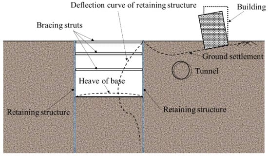
Figure 1.
Response of surrounding environment induced by an excavation.
According to engineering experience, before the strata-structure system completely fails, the system response caused by an excavation is a process of gradually increasing to stability, and there is a positive correlation among the variables in the X vector. Thus, we can deduce the relationship expression between the system response variables from Equation (1), as shown in Equation (2). The groundwater level or hydraulic head is a state variable, but considering that the change in groundwater during excavation will affect the system response, it is embodied in Equation (2).
where g(·) is the relationship function among the response variables of the system. is the vector of ground settlements. is the vector of horizontal displacements of the pile body. is the vector of horizontal displacements of the pile top. is the vector of vertical displacements of the pile top. shows the vector of the support reaction. indicates the vector of the groundwater levels or hydraulic head, which are the state variables. expresses the structure response to be determined.
Therefore, can be obtained from Equation (2) using other parameters. However, Equation (2) is not explicitly expressed and needs to be solved by an appropriate method.
2.2. Machine-Learning Technology
Machine learning is a branch of artificial intelligence and methodology which can be used to enhance potential results in terms of learning from experience. It trains and constructs a learning model based on sample data and uses the model to predict and make decisions on data, which is called inference. Nowadays, machine-learning technology has been widely used in computer vision, automatic speech recognition (ASR), natural language processing (NLP), data mining, and other fields. The classical algorithms of machine learning include support vector machines (SVM), artificial neural networks (ANNs), the AdaBoost algorithm, random forest, and so on, and SVM and ANNs are the two most widely used.
2.2.1. Support Vector Machines (SVM)
SVM is a supervised classification algorithm developed by Vapnik in 1960 s, of which the basic geometrical definition includes deciding an ideal hyperplane or plane dividing data points in the two groups or clusters and becoming equidistant, i.e., input vectors are non-linearly mapped to a high-dimension feature space. It has the advantages of good generalization performance, suitability for small samples and high-dimensional features, and non-linear data can be tackled by adding the kernel function. Now, SVM can also be applied to regression problems by introducing an alternative loss function [47]. A typical nonlinear regression structure of a support vector machine is shown in Figure 2, which is a two-layered network; the mapping function between the input layer and the first layer is nonlinear and realized through the kernel function, and the relationship between the first layer and the output layer is linear. The kernel function K(·,·) is used to map the input data into a higher dimensional feature space where linear regression is performed, and the kernel function must meet the Mercer condition, i.e., the kernel matrix needs to be positive semidefinite for any finite sample set, which obeys Equation (3). Some common kernel functions are listed in Table 1. The LIBSVM [48] is the most influential and widely used support vector machine library at present and has been integrated into the MATLAB and Python software environments. It implements five types of support vector machines for classification and regression problems, i.e., C-support vector classification (C-SVC), ν- support vector classification (ν-SVC), one-class SVM, ε-support vector regression (ε-SVR), and ν-support vector regression (ν-SVR). Thus, the LIBSVM will be employed in the following study.
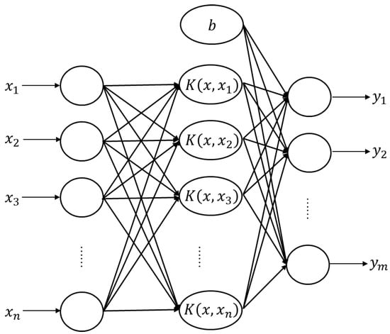
Figure 2.
Nonlinear regression structure of support vector machine.

Table 1.
Some common kernel functions.
2.2.2. Artificial Neural Networks (ANNs)
ANNs composed of an input layer, hidden layer, and output layer represent a black-box data-driven method enabling non-linear mapping between input variable sets and output variable sets without considering their physical interpretation. Of the ANNs, the BP neural network (as shown in Figure 3) is a feed-forward multilayer perceptron model using an error back-propagation learning algorithm, which has the characteristics of simplicity and high accuracy. The mapping function between adjacent layers is formed by adjusting the weight, and the nonlinearity is realized by selecting the activation function. The error back-propagation learning algorithm realizes the back-propagation of the learning method based on the error back-propagation. Figure 4 illustrates the workflow of the BP neural network algorithm. Through continuous learning with training samples, it continuously adjusts the threshold and connection weight between different layers, and finally realizes the transfer from input layer neurons to the output layer and produces the results.
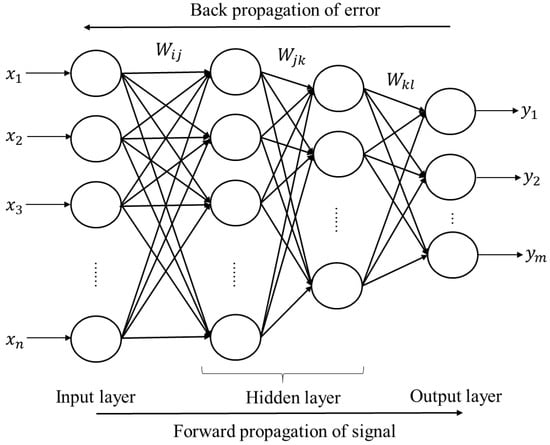
Figure 3.
A structure diagram of a BP neural network.
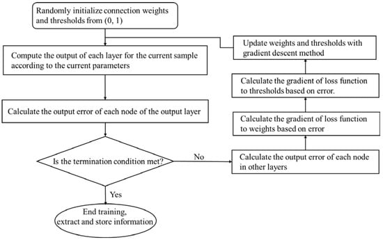
Figure 4.
The workflow of a BP neural network algorithm.
2.3. Implementation of a Data-Driven Prediction Approach Based on Machine Learning
In general, after defining the input variables and the output variables in Equation (2), the relationship between inputs and outputs can be sought by using the SVM or the BP neural network. However, the machine-learning-based model constructed should have pertinence to the construction method in view of the difference of monitoring items for the cut-and-cover method, shallow-mining method, and shield-tunneling method, etc. The monitoring data need to be pre-processed before establishing the machine-learning model due to the difference in measurement units of the monitoring data. Thus, taking the construction of the machine-learning-based model for predicting the deformation of existing buildings induced by adjacent excavation of a foundation pit as an example, the framework of the data-driven prediction approach based on machine learning is expounded on in this section.
Excavation is often accompanied with the uplift of the stratum at the bottom of the foundation pit, the deformation of the retaining structure, and the movement of the stratum around the foundation pit, which will cause the deformation of the surrounding existing buildings and affect their safety. The technical code for the monitoring of building foundation pit engineering (GB50497–2019) [46] recommends the monitoring items of foundation pit engineering according to the safety grade of excavation, as listed in Table 2. In general, some items, such as horizontal displacement at the top of the retaining structure/slope, vertical displacement at the top of the retaining structure/slope, subsurface horizontal displacement, the axial force of bracing/axial load of the anchor bolt, hydraulic head, and ground vertical displacement, must be monitored during excavation. Thus, the monitored items above can be selected as the input variables of a prediction model. Table 3 lists the variables of the prediction model in this article. As shown in Table 3, the measurement units of these variables are different. Meanwhile, each variable is a spatial and temporal variable with different values at a different location and different time. In order to facilitate the construction of the prediction model and reduce the amount of calculation, it is necessary to normalize the model variables and reduce the dimensions of the model variables.
Table 2.
Instrument monitoring items of soil mass excavation (GB50497–2019).
Table 3.
The variables of the prediction model.
2.3.1. Dimensionality Reduction of Variable Data
The monitoring points are arranged in the whole area affected by excavation, and the monitoring results of each point are controlled by its location and excavation process. In order to reduce the calculation time required for model construction and improve the operation speed, it is an effective method to weight the monitoring results according to the importance of the monitoring points and establish equivalent monitoring variables, so as to reduce the dimensions of the variable data.
- Ground vertical displacement
Ground vertical displacement (i.e., ground subsidence) is an important manifestation caused by excavation and a problem of great concern. Ground subsidence induced by excavation has been deeply studied by some scholars. For example, Kung et al., (2007) [49] proposed a simplified semi-empirical model for predicting maximum surface settlement and the surface-settlement profile due to excavation in soft to medium clays. Xiao et al., (2019) [8] found that the maximum ground settlements first increase and then tend to stable with the increase in excavation width. Mu and Huang (2013) [50] generalized the attenuation laws of the soil movement behind the wall (as shown in Figure 5) and proposed a simplified method to calculate the soil movement induced by excavation, as shown in Equations (4)–(8).
where umax is the maximum horizontal displacement of the retaining wall. L is the excavation length of the foundation pit along the retaining wall. H is the excavation depth of the foundation pit.
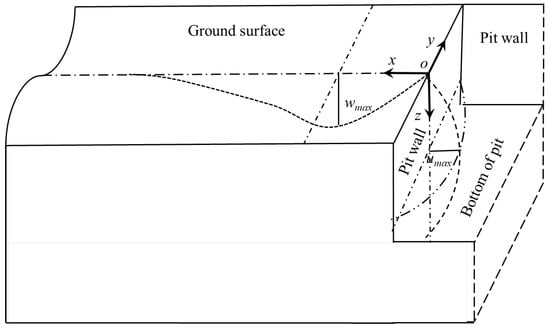
Figure 5.
Schematic diagram of deformations of wall and soils induced by excavation.
According to engineering experience, the larger the value of the ground subsidence, the greater the security risk in excavation of a foundation pit. Therefore, it can be defined as follows: the greater the value, the greater the weight of the monitoring point. After the coordinate origin of ground settlement analysis is determined according to the position of the maximum horizontal displacement of the retaining wall, the corresponding position coordinates of monitoring points for ground settlement can be determined, their respective weights can be determined with according to Equation (4), and the weighted average of the monitoring values at all monitoring points is the equivalent ground settlement.
- 2.
- Subsurface horizontal displacement/Deflection of the retaining structure
Zheng et al., (2021) [51] investigated the mechanism of the vertical progressive collapse of deep excavations retained by a multilayer strutting system and found that when the maximum bending moment exceeds the ultimate bending capacity, the diaphragm wall will rupture, resulting in the overall collapse of the excavation. Deflection of the retaining structure is positively correlated with its bending moment, reflects the exertion level of the resistance of the retaining structure, and indicates the damage degree of the foundation pit. Thus, the maximum monitored horizontal displacement in each stage is taken as the equivalent displacement of the retaining structure in this study, considering that the failure process of excavation is a progressive failure.
- 3.
- Axial force of bracing/anchor bolts
Previous studies have shown that the failure of excavation begins with the failure of the struts or anchor bolt [51,52]. The earth pressure on the retaining structures at different depths is different, so the importance of bracing/anchor bolts at different depths is also different; thus, it is recommended to use the design control values of bracing/anchor bolts at different depths to divide the weight of bracing or anchor bolts in the study, which is called the depth weight. After taking the average value of the axial force of bracing/anchor bolts at the same depth, the equivalent axial force of bracing/anchor bolts is obtained by weighting the average value with the depth weight.
- 4.
- Vertical/horizontal displacement at the top of the retaining structure/slope
Similar to the treatment method for deflection of retaining structure, the maximum value of vertical/horizontal displacement at the top of retaining structure/slope of the current period is taken as the equivalent vertical/horizontal displacement at the top of retaining structure by adopting the maximum envelope principle.
- 5.
- Vertical displacement of the column
The vertical displacement of the column leads to the eccentricity of bracing, which affects the stability of bracing. In this study, the average value of the monitoring results is used as the equivalent vertical displacement of the column.
- 6.
- Hydraulic head/Groundwater table
Hydraulic head/groundwater table is a field variable during excavation. In order to ensure safety and the anhydrous operation of excavation, dewatering and waterproof curtains are usually required to control the groundwater. The change in hydraulic head/groundwater table will inevitably change the stress field of the site. Therefore, it is necessary to monitor the change in hydraulic head during excavation to ensure that it is within a controllable range. In this study, the lowest hydraulic head, i.e., the monitoring value at the maximum drawdown depth of hydraulic head, is used as the equivalent hydraulic head.
- 7.
- Vertical displacement of surrounding buildings
The responses of existing buildings are an issue of great concern in excavation. In this study, the settlement of existing buildings adjacent to excavation is selected as the research object, i.e., the output variable. In order to better predict this, the maximum envelope principle is used to deal with the on-site monitoring results—that is, the maximum cumulative settlement of the measuring points in the current period is taken as the equivalent settlement of the surrounding buildings.
2.3.2. Normalization of Variable Data
As we know, different monitoring items use different measurement units, as shown in Table 3. In order to seek the relationship among the variables in Equation (2), it is necessary to normalize these variables first, so as to eliminate the restrictions caused by the difference in the measurement units of the data and convert them into dimensionless pure values. There are two normalization methods. The first is to normalize the monitoring results by using the design limits (i.e., control values) for specific projects, which must be implemented before constructing equivalent variables. Since the control value set for the specific project has a large subjective nature and cannot cover the actual monitoring results, the normalized results by this method cannot be guaranteed to be within the range of [−1,1]. The second method is to consider the characteristics of the data and adopt mathematical statistical methods to normalize the monitoring data, and some normalization functions have been implemented in MATLAB [53] including the premnmx function, tramnmx function, postmnmx function, mapminmax function, and prestd function, etc. Among which, the mapminmax function can be used to realize the normalization of data and the restore of normalized data. Thus, the normalization function of mapminmax in MATLAB is directly used for data preprocessing in this article.
2.3.3. Prediction Model Based on Machine Learning
When the inputs and outputs in Equation (2) are selected and preprocessed by the above method, the corresponding prediction model can be constructed with machine-learning technology. Figure 6 shows the implementation process of a prediction model based on machine-learning technology for the settlement of existing buildings surrounding an excavation site, which we have implemented in MATLAB.
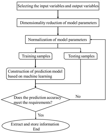
Figure 6.
Implementation process of prediction model based on machine learning.
3. Validation of the Proposed Method
3.1. Project Overview
Excavation engineering for the Central Hospital Station of Xuzhou Rail Transit Line 2 is used to verify the feasibility of the proposed method. The station is a two-story underground station with an island platform. The main standard section is a double-layer, double span, single column box type frame structure. The cut-and-cover method is adopted, the total length of the excavation is 237.20 m, and the standard section is 21.7 m × 16.59 m (width × depth). Row piles and inner bracing are employed to maintain the stability in excavation. The commercial building on the west side of the station is the existing building closest to the excavation with a distance of 16.12 m from the main body of the station; thus, the settlement of this building caused by excavation will be used to verify the proposed method in this article.
Figure 7 shows the relative position of the commercial building and the excavation. The monitoring items include the vertical displacement of the building, the ground vertical displacement, the deflection of the retaining structure, the vertical displacement at the top of the retaining structure, the horizontal displacement at the top of the retaining structure, the axial force of bracing, the vertical displacement of the column, and the groundwater table. The foundation pit is excavated from north to south, as indicated by the serial numbers of ① to ⑩ in Figure 7.
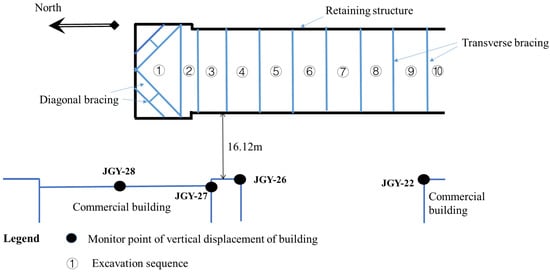
Figure 7.
Position of the buildings and the excavation.
In this section, the monitoring data from 17 May 2017 to 16 June 2017 are selected for analysis. The area involved in this excavation process covers ① to ⑥. Among this area, the excavation depths of ① to ② are 11.0 m–15.0 m and those of ③ to ⑥ are 7.0 m–9.0 m, the area from ⑦ to ⑩ is the route of the muck truck which is simply sloping without support and the excavation depth is shallow. During analysis, the excavation process is divided into 31 issues according to the daily reports; thus, we obtain 31 groups of original sample data. Figure 8 shows the history curve of building settlement, which indicates that the settlement values of different positions on the building are different, but the settlements increase with the advance of excavation.
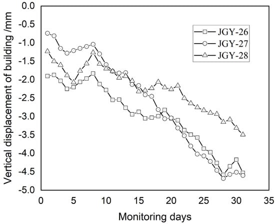
Figure 8.
History curve of building settlement.
3.2. Prediction of Settlement of Existing Building Induced by Excavation
3.2.1. Evaluation Index for Prediction Model
In this article, the mean absolute percentage error (MAPE) and the coefficient of determination (denoted by R2) are employed to evaluate the accuracy and applicability of the proposed data-driven model in predicting the settlement of the building.
The definition of MAPE is shown in Equation (9). The smaller the MAPE value, the better the model. That is, MAPE = 0% indicates that the model is perfect, and MAPE≈100% means that the model is inferior.
where, n is the sequence length.
The coefficient of determination (R2), as shown in Equation (10), is used to evaluate the consistency between the predicted results and the measured results, which is interpreted as the proportion of the variance in the dependent variable that is predictable from the independent variable. A high R2 value indicates that the model is a good fit for the data.
where, n is the sequence length.
3.2.2. Prediction Based on the SVM Model
The LIBSVM toolbox with the RBF kernel function is employed in this study. From the original sample data, 24 groups of sample data are randomly selected as training samples to form training sets, and the remaining 7 groups of sample data are taken as testing samples to form testing sets. Based on the data of the training sets, the parameter of the error penalty factor (c) and the kernel function parameter (γ) are optimized using a cross-validation technique and grid-search method under the tolerance of a termination criterion of epsilon equal to 0.001. Figure 9a shows the building settlement predicted by the optimized parameters obtained from the data of the training sets. Compared with the equivalent settlement of the building, the MAPE of the prediction by the SVM model is 8.6889% and the R2 is 0.86497, which indicate that the prediction model based on SVM is a good fit for the data.
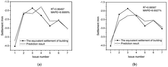
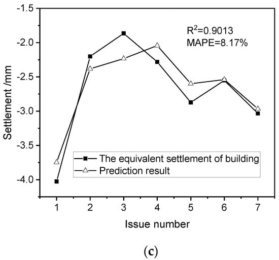
Figure 9.
The settlement of buildings predicted by a machine-learning-based model; (a) SVM model; (b) BP model; (c) BP–SVM model.
3.2.3. Prediction Based on the BP Model
For the same training sets and testing sets, a single hidden layer BP neural network is used to find the relationship between the inputs and outputs. The number of nodes in the input layer is 7 and the number of nodes in the output layer is 1. The sigmoid function is used as the activation function of the hidden layer, and the activation function of the output layer is linear. In order to obtain a faster training speed and improve output accuracy, the number of nodes in the hidden layer is 11. The initial weight is a random number between [−1, 1]. The learning rate is taken as 0.1, the expected error is 0.001, and the gradient descent method is adopted as the training algorithm. Figure 9b shows that the predicted value is in good agreement with the equivalent settlement of the building: the MAPE of the prediction by BP model is 8.6927% and the R2 is 0.88567.
3.3. Discussions
Figure 9a,b show that good prediction results can be obtained using the settlement prediction method proposed in this article, which means that the proposed approach is reasonable and feasible. However, due to the operation difference between SVM and BP neural networks, the results obtained by the two models are different. The maximum difference between the prediction results based on SVM model and the equivalent settlement of the building occurs in the fourth issue of the testing sets: the maximum difference value is 0.4817 mm. However, the maximum difference between the prediction results based on the BP model and the equivalent settlement of the building appears in the third issue of the testing sets: the maximum difference value is −0.4161 mm. Therefore, in order to minimize the impact caused by the deficiency of the BP neural network and SVM in the prediction process, it is suggested to assign different weights to the BP neural network and SVM according to game theory [54] and combine the BP neural network and SVM for prediction, which is called the BP–SVM model. The construction of the BP–SVM model is shown in Equation (11).
Subject to the constraints: , where, x is the combined predicted value, xi is the predicted value obtained by the ith algorithm, ωi is the weight of the ith algorithm and , and n is the number of algorithms.
Assuming that the prediction error of the ith algorithm is (i represents the ith algorithm, t represents the issue number), the prediction error of the combined prediction method is , .
The objective function M is constructed as
where, , , , and
Taking matrix R as n × 1, , the
Then, the optimal weighting coefficient vector W can be obtained from Equation (13).
Based on the above predicted results from the SVM model and BP model, the corresponding prediction errors are obtained, and according to the optimal weight criterion, the optimal weights ωSVM and ωBP are gained, which are 0.4444 and 0.5556. Figure 9c shows the building settlement predicted by the BP–SVM model. Comparing Figure 9a–c, it is found that the results predicted by the BP–SVM model are closer to the real results. According to the MSPE and the R2, the BP–SVM model effectively reduces the difference fluctuation, improves the utilization of data, enhances the reliability of the prediction model, and improves the accuracy of the prediction results compared with the single algorithms.
In addition to gradually increasing with the advance of excavation, the settlement of existing buildings is also related to the plane position and the excavation process. Generally, the settlement of buildings facing the middle of excavation is large. Thus, the proposed approach is also used to predict the settlement of another building at JGY-22. There are two purposes: (i) to discuss the prediction accuracy when the training sets and testing sets are divided according to the construction sequence; (ii) to analyze the prediction accuracy of the proposed model under large excavation. The data used in this study are the monitoring data from the 70th to the 180th day of excavation. Among them, the data of the first 80 days (i.e., from the 70th to the 150th day) are the training samples, the data of the middle 23 days (i.e., from the 151st to the 173rd day) are the testing samples, and the data of the last 7 days (i.e., from the 174th to the 180th day) are used as the prediction samples.
Figure 10 shows the prediction results for the settlement of buildings at JGY-22, using the SVM model, the BP model, and the BP–SVM model. It is found that the variation trends of the predicted results are consistent with the measured results, and the prediction accuracy of BP–SVM model is higher than that of the other two models. The prediction accuracy for the prediction samples is lower than that of the testing samples, but the values of R2 are all greater than 0.6 which is acceptable in the project. Figure 11 presents the history curve of R2, which indicates that the accuracy of prediction results decreases for long-term prediction with the advance of excavation, but it will gradually tend to stable.
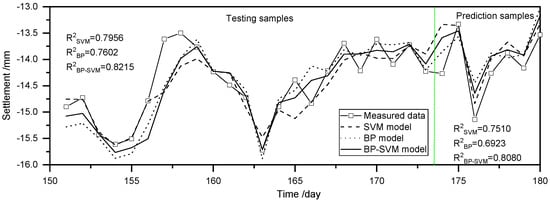
Figure 10.
Prediction results for the settlement of building at JGY-22.
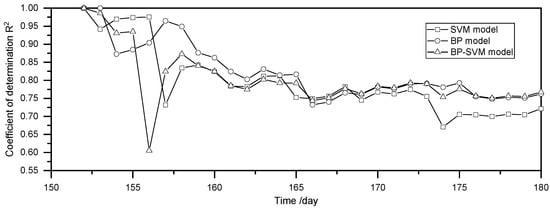
Figure 11.
History curve of R2.
The above results demonstrate that the proposed method can be used as a supplement to field monitoring to predict the response of existing buildings induced by excavation, and the prediction accuracy is related to the machine-learning algorithm used. Meanwhile, the data of training samples needs to be updated continuously according to the excavation process in order to make better predictions, due to the fact that the model obtained through training sets is an approximate solution and the model parameters will change with the advancement of excavation.
4. Conclusions
In this article, the feasibility of making full use of on-site monitoring data to predict the mechanical response of existing structures adjacent to excavation is discussed. By analyzing the mechanical response of the surrounding environment induced by excavation, a data-driven indirect method to predict the response of adjacent existing structures is constructed, which makes full use of the monitoring data of items which must be monitored and is realized by using the SVM algorithm and the BP neural network algorithm. In contrast with the prediction method proposed in the previous literature, the proposed method avoids complex mechanical calculations and directly uses the monitoring data of the items required by the specification to make indirect predictions, which is convenient for engineering applications and can be used as a supplement to field monitoring in order to predict the response of existing buildings induced by adjacent excavation. Simultaneously, the machine-learning algorithms have a significant impact on the accuracy of the prediction results and the proposed approach can be implemented by using other machine-learning algorithms: specific investigation will be carried out in the future.
Further, for the response of concealed structures induced by excavation that cannot be directly monitored, similar schemes can be adopted whereby the training set data can be obtained by numerical simulation, in which the numerical model parameters need to be obtained through inversion using on-site monitoring data.
Author Contributions
Conceptualization, L.L. and Q.S.; methodology, L.L. and Q.S.; software, Q.S.; validation, L.L., Q.S. and Y.W.; formal analysis, Q.S.; investigation, Q.S. and Y.G.; resources, Q.S. and Y.G.; data curation, Q.S.; writing—original draft preparation, Q.S. and L.L.; writing—review and editing, L.L.; visualization, Q.S.; supervision, L.L.; project administration, Y.W.; funding acquisition, L.L. and Y.W. All authors have read and agreed to the published version of the manuscript.
Funding
This research was funded by the Beijing Municipal Science and Technology Planning Project, grant number Z181100009018001 and the Beijing Postdoctoral Research Foundation, grant number 2021 zz-104.
Institutional Review Board Statement
Not applicable.
Informed Consent Statement
Not applicable.
Data Availability Statement
All data, models, and code generated or used during the study appear in the submitted article.
Conflicts of Interest
The authors declare no conflict of interest.
References
- Ou, C.Y.; Chiou, D.C.; Wu, T.S. Three-dimensional Finite Element Analysis of Deep Excavations. J. Geotech. Eng. 1996, 122, 337–345. [Google Scholar] [CrossRef]
- Finno, R.J.; Blackburn, J.T.; Roboski, J.F. Three-Dimensional Effects for Supported Excavations in Clay. J. Geotech. Geoenviron. Eng. 2007, 133, 30–36. [Google Scholar] [CrossRef]
- Hsiung, B.-C.B.; Yang, K.-H.; Aila, W.; Hung, C. Three-dimensional effects of a deep excavation on wall deflections in loose to medium dense sands. Comput. Geotech. 2016, 80, 138–151. [Google Scholar] [CrossRef]
- Mu, L.; Huang, M. Small strain based method for predicting three-dimensional soil displacements induced by braced excavation. Tunn. Undergr. Space Technol. 2016, 52, 12–22. [Google Scholar] [CrossRef]
- Dan, K.; Sahu, R.B. Estimation of Ground Movement and Wall Deflection in Braced Excavation by Minimum Potential Energy Approach. Int. J. Geomech. 2018, 18, 04018068. [Google Scholar] [CrossRef]
- Lim, A.; Ou, C.Y. Performance and Three-Dimensional Analyses of a Wide Excavation in Soft Soil with Strut-Free Retaining System. Int. J. Geomech. 2018, 18, 05018007. [Google Scholar] [CrossRef]
- Tan, Y.; Lu, Y.; Xu, C.; Wang, D. Investigation on performance of a large circular pit-in-pit excavation in clay-gravel-cobble mixed strata. Tunn. Undergr. Space Technol. 2018, 79, 356–374. [Google Scholar] [CrossRef]
- Xiao, H.; Zhou, S.; Sun, Y. Wall Deflection and Ground Surface Settlement due to Excavation Width and Foundation Pit Classification. KSCE J. Civ. Eng. 2019, 23, 1537–1547. [Google Scholar] [CrossRef]
- Li, L.; Du, X.; Zhou, J. Numerical Simulation of Site Deformation Induced by Shield Tunnelling in Typical Upper-Soft-Lower-Hard Soil-Rock Composite Stratum Site of Changchun. KSCE J. Civ. Eng. 2020, 24, 3156–3168. [Google Scholar] [CrossRef]
- Sun, Y.; Xiao, H. Wall Displacement and Ground-Surface Settlement Caused by Pit-in-Pit Foundation Pit in Soft Clays. KSCE J. Civ. Eng. 2021, 24, 1262–1275. [Google Scholar] [CrossRef]
- Wang, S.; Li, Q.; Dong, J.; Wang, J.; Wang, M. Comparative investigation on deformation monitoring and numerical simulation of the deepest excavation in Beijing. Bull. Eng. Geol. Environ. 2020, 80, 1233–1247. [Google Scholar] [CrossRef]
- Yahya, S.M.; Abdullah, R.A. A Review on Methods of Predicting Tunneling Induced Ground Settlements. Electron. J. Geotech. Eng. 2014, 19, 5813–5826. [Google Scholar]
- Zhao, X.D.; Zhou, G.Q.; Qiao, L.J.; Chen, Y. Behaviors of Wall and Ground due to T-shaped Excavation. KSCE J. Civ. Eng. 2019, 23, 1999–2008. [Google Scholar] [CrossRef]
- Zhang, Z.; Zhang, M.; Jiang, Y.; Bai, Q.; Zhao, Q. Analytical prediction for ground movements and liner internal forces induced by shallow tunnels considering non-uniform convergence pattern and ground-liner interaction mechanism. Soils Found. 2017, 57, 211–226. [Google Scholar] [CrossRef]
- Finno, R.J.; Bryson, L.S. Response of building adjacent to stiff excavation support system in soft clay. J. Perform. Constr. Facil. 2002, 16, 10–20. [Google Scholar] [CrossRef]
- Finno, R.J.; Voss, F.T.; Rossow, E.; Blackburn, J.T. Evaluating damage potential in building affected by excavations. J. Geotech. Geoenviron. Eng. 2005, 131, 1199–1210. [Google Scholar] [CrossRef]
- Laefer, D.F.; Ceribasi, S.; Long, J.H.; Cording, E.J. Predicting RC Frame Response to Excavation-Induced Settlement. J. Geotech. Geoenviron. Eng. 2009, 135, 1605–1619. [Google Scholar] [CrossRef]
- Schuster, M.; Kung, G.T.-C.; Juang, C.H.; Hashash, Y.M.A. Simplified Model for Evaluating Damage Potential of Buildings Adjacent to a Braced Excavation. J. Geotech. Geoenviron. Eng. 2009, 135, 1823–1835. [Google Scholar] [CrossRef]
- Kog, Y.C. Buried Pipeline Response to Braced Excavation Movements. J. Perform. Constr. Facil. 2010, 24, 235–241. [Google Scholar] [CrossRef]
- Bryson, L.S.; Kotheimer, M. Cracking in Walls of a Building Adjacent to a Deep Excavation. J. Perform. Constr. Facil. 2011, 25, 491–503. [Google Scholar] [CrossRef]
- Juang, C.H.; Schuster, M.; Ou, C.-Y.; Phoon, K.K. Fully Probabilistic Framework for Evaluating Excavation-Induced Damage Potential of Adjacent Buildings. J. Geotech. Geoenviron. Eng. 2011, 137, 130–139. [Google Scholar] [CrossRef]
- Castaldo, P.; Callvello, M.; Palazzo, B. Probabilistic analysis of excavation-induced damages to existing structures. Comput. Geotech. 2013, 53, 17–30. [Google Scholar] [CrossRef]
- Huang, X.; Schweiger, H.F.; Huang, H. Influence of Deep Excavations on Nearby Existing Tunnels. Int. J. Geomech. 2013, 13, 170–180. [Google Scholar] [CrossRef]
- Ng, C.W.; Shi, J.; Hong, Y. Three-dimensional centrifuge modelling of basement excavation effects on an existing tunnel in dry sand. Can. Geotech. J. 2013, 50, 874–888. [Google Scholar] [CrossRef]
- Mu, L.; Chen, W.; Huang, M.; Lu, Q. Hybrid Mehtod for Predicting the Response of a Pile-Raft Foundation to Adjacent Braced Excavation. Int. J. Geomech. 2020, 20, 04020026. [Google Scholar] [CrossRef]
- Xu, R.; Shen, S.; Dong, M.; Cheng, K. A Simplified Calculation Method for Vertical Displacement of Shield Tunnel Caused by Adjacent Excavation. Geotech. Geol. Eng. 2020, 39, 2269–2286. [Google Scholar] [CrossRef]
- Zheng, G.; Pan, J.; Li, Y.; Cheng, X.; Tan, F.; Du, Y.; Li, X. Deformation and Protection of Existing Tunnels at an Oblique Intersection Angle to an Excavation. Int. J. Geomech. 2020, 20, 05020004. [Google Scholar] [CrossRef]
- Meng, F.-Y.; Chen, R.-P.; Liu, S.-L.; Wu, H.-N. Centrifuge Modeling of Ground and Tunnel Responses to Nearby Excavation in Soft Clay. J. Geotech. Geoenviron. Eng. 2021, 147, 04020178. [Google Scholar] [CrossRef]
- Meng, F.-Y.; Chen, R.-P.; Xu, Y.; Wu, K.; Wu, H.-N.; Liu, Y. Contributions to responses of existing tunnel subjected to nearby excavation: A review. Tunn. Undergr. Space Technol. 2022, 119, 104195. [Google Scholar] [CrossRef]
- Peck, R.B. Deep excavations and tunnelling in soft ground. In Proceedings of the 7th International Conference on Soil Mechanics and Foundation Engineering, Mexico City, Mexico, 29 August 1969; pp. 225–290. [Google Scholar]
- Zheng, H.B.; Li, P.F.; Ma, G.W.; Zhang, Q.B. Experimental investigation of mechanical characteristics for linings of twins tunnels with asymmetric cross-section. Tunn. Undergr. Sp. Technol. 2022, 119, 104209. [Google Scholar] [CrossRef]
- Tang, L.; Na, S. Comparison of machine learning methods for ground settlement prediction with different tunneling datasets. J. Rock Mech. Geotech. Eng. 2021, 13, 1274–1289. [Google Scholar] [CrossRef]
- Zhang, N.; Zhou, A.; Pan, Y.; Shen, S.-L. Measurement and prediction of tunnelling-induced ground settlement in karst region by using expanding deep learning method. Measurement 2021, 183, 109700. [Google Scholar] [CrossRef]
- Liu, L.; Zhou, W.; Gutierrez, M. Effectiveness of predicting tunneling-induced ground settlements using machine learning methods with small datasets. J. Rock Mech. Geotech. Eng. 2022, 14, 1028–1041. [Google Scholar] [CrossRef]
- Ye, X.; Jin, T.; Chen, Y. Machine learning-based forecasting of soil settlement induced by shield tunneling construction. Tunn. Undergr. Space Technol. 2022, 124, 104452. [Google Scholar] [CrossRef]
- Ling, X.; Kong, X.; Tang, L.; Zhao, Y.; Tang, W.; Zhang, Y. Predicting earth pressure balance (EPB) shield tunneling-induced ground settlement in compound strata using random forest. Transp. Geotech. 2022, 35, 100771. [Google Scholar] [CrossRef]
- Ling, X.; Kong, X.; Tang, L.; Zhao, Y.; Tang, W.; Zhang, Y. Spatical-temporal fusion network for maximum ground surface settlement predication during tunnel excavation. Autom. Constr. 2023, 147, 104732. [Google Scholar] [CrossRef]
- Zhou, X.; Zhao, C.; Bian, X. Prediction of maximum ground surface settlement induced by shield tunneling using XGBoost algorithm with golden-sine seagull optimization. Comput. Geotech. 2023, 154, 105156. [Google Scholar] [CrossRef]
- Kim, D.; Kwon, K.; Pham, K.; Oh, J.-Y.; Choi, H. Surface settlement prediction for urban tunneling using machine learning algorithms with Bayesian optimization. Autom. Constr. 2022, 140, 104331. [Google Scholar] [CrossRef]
- Zhao, H.; Liu, W.; Guan, H.; Fu, C. Analysis of diaphragm wall deflection induced by excavation based on machine learning. Math. Probl. Eng. 2021, 2021, 6664409. [Google Scholar] [CrossRef]
- Mu, L.; Lin, J.; Shi, Z.; Kang, X. Predicting excavation-induced tunnel response by process-based modelling. Complexity 2020, 2020, 9048191. [Google Scholar] [CrossRef]
- Feng, T.; Wang, C.; Zhang, J.; Wang, B.; Jin, Y.-F. An improved artificial bee colony-random forest (IABC-RF) model for predicting the tunnel deformation due to an adjacent foundation pit excavation. Undergr. Space 2022, 7, 514–527. [Google Scholar] [CrossRef]
- Zhang, D.; Shen, Y.; Huang, Z.; Xie, X. Auto machine learning-based modelling and prediction of excavation-induced tunnel displacement. J. Rock Mech. Geotech. Eng. 2022, 14, 1100–1114. [Google Scholar] [CrossRef]
- Nguyen, D.; Kim, D.; Choo, Y. Optimized extreme gradient boosting machine learning for estimating diaphragm wall deflection of 3D deep braced excavation in sand. Structures 2022, 45, 1936–1948. [Google Scholar] [CrossRef]
- Pan, Y.; Zhang, L. Mitigating tunnel-induced damages using deep neural networks. Autom. Constr. 2022, 138, 104219. [Google Scholar] [CrossRef]
- GB50497-2019; Technical Code for Monitoring of Building Excavation Engineering. Ministry of Housing and Urban-Rural Development of the People’s Republic of China (MOHURD): Beijing, China, 2019. (In Chinese)
- Dibike, Y.B.; Velickov, S.; Solomatine, D.; Abbott, M.B. Model Induction with Support Vector Machnies: Introduction and Applications. ASCE J. Comput. Civ. Eng. 2001, 15, 208–216. [Google Scholar] [CrossRef]
- Chang, C.C.; Lin, C.J. LIBSVM: A library for support vector machines. ACM Trans. Internet Syst. Technol. 2011, 2, 1–27. [Google Scholar] [CrossRef]
- Kung, G.T.; Juang, C.H.; Hsiao, E.C.; Hashash, Y.M. Simplified Model for Wall Deflection and Ground-Surface Settlement Caused by Braced Excavation in Clays. J. Geotech. Geoenviron. Eng. 2007, 133, 731–747. [Google Scholar] [CrossRef]
- Mu, L.; Huang, M. Simplified Method for Analysis of Soil Movement Induced by Excavations. Chin. J. Geotech. Eng. 2013, 35, 820–827. (In Chinese) [Google Scholar]
- Zheng, G.; Zhao, J.; Cheng, X.; Yu, D.Y.; Wang, R.Z.; Zhu, X.W.; Yi, F. Mechanism and Control Measures of the Vertical Progressive Collapse of Deep Excavations Retained by a Multilayer Strutting System. J. Tianjin Univ. (Sci. Technol.) 2021, 54, 1025–1038. (In Chinese) [Google Scholar]
- Zheng, G.; Lei, Y.; Cheng, X.; Li, X.Y.; Wang, R.Z. Experimental study on the progressive collapse mechanism in the braced and tied-back retaining systems of deep excavations. Can. Geotech. J. 2020, 58, 540–564. [Google Scholar] [CrossRef]
- Paluszek, M.; Thomas, S. MATLAB Machine Learning; Apress Media: Berlin/Heidelberg, Germany, 2017. [Google Scholar] [CrossRef]
- Tadelis, S. Game Theory—An Introduction; Princeton University Press: Princeton, NJ, USA, 2013; ISBN 978-0-6911-2908-2. [Google Scholar]
Disclaimer/Publisher’s Note: The statements, opinions and data contained in all publications are solely those of the individual author(s) and contributor(s) and not of MDPI and/or the editor(s). MDPI and/or the editor(s) disclaim responsibility for any injury to people or property resulting from any ideas, methods, instructions or products referred to in the content. |
© 2023 by the authors. Licensee MDPI, Basel, Switzerland. This article is an open access article distributed under the terms and conditions of the Creative Commons Attribution (CC BY) license (https://creativecommons.org/licenses/by/4.0/).