Abstract
Glass products are important evidence of early East–West cultural exchanges. Ancient glass in China mostly consisted of lead glass, and potassium glass is widely believed to be imported abroad. In order to figure out the origin of glass artefacts, it is crucial to define the type of glass products accurately. In contemporary research on the chemical composition of ancient glass products, potassium glass is separated from lead glass primarily by the weight ratio of oxides or the proportion of lead-containing compounds. This approach can be excessively subjective and prone to mistakes while calculating the mass fraction of compounds containing potassium. So, it is better to find out the link between the proportion of glass’s chemical composition and its classifications during the weathering process of the glass products, to develop an effective classification model using machine learning techniques. In this research, we suggest employing the slime mould approach to optimise the parameters of a support vector machine and examine a 69-group glass chemical composition dataset. In addition, the results of the proposed algorithm are compared to those of commonly used classification models: decision trees (DT), random forests (RF), support vector machines (SVM), and support vector machines optimised by genetic algorithms (GA-SVM). The results of this research indicated that the support vector machine method with the sticky slime mould algorithm strategy is the most effective. On the training set, 100% accuracy was attained, while on the test set, 97.50% accuracy was attained in this research. The research results demonstrate that the support vector machine algorithm combining the slime mould algorithm strategy is capable of providing a trustworthy classification reference for future glass artefacts.
1. Introduction
Glass is a special type of silicate product. The development, manufacturing, distribution, and use of glass have been crucial to the study of the history of human civilisation, particularly the history of early civilisations. The first manufacturing of ancient glass in China developed from the creation of porcelain glazes from primitive porcelain. The determination and analysis of the chemical composition of the elements are vital for the study of ancient glass artefacts and may provide much information about the beginnings of glass, the types of raw materials and sources, the history of fire techniques, and the dissemination of products. The classification of glass artefacts can reveal potential trade relations and cultural exchanges between different regions in ancient times. Future researchers can delve deeper and more accurately infer and complete ancient trade networks and cultural exchange patterns based on the classification results.
In 1798, the German scientist M.H. Klaproth conducted the first quantitative chemical study of three Roman-era glass mosaics. The chemical analysis of Chinese glass artefacts dates back to 2003 when a group led by academician Fuxi Gan analysed the chemical composition of a group of ancient Chinese glasses using proton-excited X-ray fluorescence techniques. Fuxi Gan’s objective was to investigate the old glass composition system, the age of manufacturing, the preparation method, and the genesis of the technology.
With the increasing research on ancient silicate artefacts, many scholars began to try to classify ancient artefacts according to their chemical composition. In 1992, Lee Chul, a Korean scientist, analysed the chemical composition of 94 ancient Korean glass fragments using principal component analysis and other methods and attempted to classify them [1]. In 2002, Yoon Yeol Yoon conducted an elemental analysis using INAA and XRF methods. In the elemental analysis, some rare earth elements with different regional characteristics were used to classify ancient Korean ceramics [2]. In 2011, K. Baert et al. highlighted the great potential of Raman spectroscopy as a rapid screening method for a large number of ancient glass samples [3]. In 2019, Nadine Schibille et al. developed a temporal model as a tool for the dating of archaeological glass assemblages, as well as a geographical model that allows for the unambiguous classification of phyllo-grey glasses from the Levant region and Egypt [4]. However, to date, there has been very little discussion of studies that have used machine learning to classify ancient glassworks.
In recent years, when studying the chemical composition of ancient glass products, the classification of glass is still mostly judged by the weight ratio of oxides or by analysing the mass fraction of lead- and potassium-containing compounds when researching the chemical composition of ancient glass items [5,6,7,8]. However, due to the glass production area and weathering degree, the proportion of lead-containing and potassium-containing compounds are different, which will interfere with the classification of glass. Therefore, a new method should be proposed to more accurately classify glass artefacts in terms of the proportion of their chemical composition. Common directions for improvement are to propose a new architecture [9,10], a new algorithm [11], or to combine multiple existing approaches.
Machine learning models, such as decision tree models (DT) [12,13], random forest models (RF) [14], K-nearest neighbour algorithm models (KNN) [15,16], artificial neural network models (ANN) [17,18,19,20], and support vector machine models (SVM) [21], have been proposed and widely used in classification research as a result of the continuous development of machine learning techniques [22,23]. Traditional machine learning approaches have significant drawbacks in addressing real-world issues, including not always meeting scientific standards [24], unsupervised training of input data, and poor prediction accuracy. It is required to combine classic machine learning methods with more sophisticated approaches to increase the accuracy of glass classification, such as heuristic algorithms and large data analysis. This combines the slime mould method from the heuristic algorithm with support vector machines from the optimisation theory. The parameters of the support vector machine are optimised and used for the categorisation of ancient glass artefacts using the slime mould approach (Figure 1). Using an examination of the dataset supplied for the 2022 China Undergraduate Mathematical Contest in Modeling, this study demonstrates the correctness of the suggested approach.
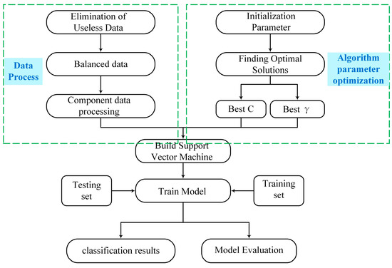
Figure 1.
Experimental Process.
The primary contributions of this study include the following:
- An excellent classification model for glass artefact kinds has been identified;
- We incorporate the slime mould algorithm strategy into a support vector machine model and provide a parameter-optimisation strategy for support vector machines;
- We compare the multiple categorisation models, and the experimental findings demonstrate the superiority of the algorithmic approach provided in this study;
- The model is applicable to additional glass artefact samples.
This article contains five parts: The processing of the data utilised in this study is discussed in the second section. In the third section, the algorithmic model suggested in this paper is described in depth. In the fourth section, experimental data and model performance comparisons are presented. Part five concludes with conclusions and suggested future studies.
2. Materials and Methods
2.1. Datasets
This study’s dataset is comprised of data from the 2022 China Undergraduate Mathematical Contest in Modeling. The data collection includes 69 data sets regarding the chemical composition of glass artefacts. Each data set includes the artefact number, the artefact type, and percentage statistics for 14 oxide components. Due to a large number of features and the large order-of-magnitude differences between the data, missing data, and errors, it is necessary to pre-process the information contained in the 69 sets of glass artefact data to ensure the credibility and interpretability of the data and to prevent incorrect data from affecting the processing results. There are 20 sets of potassium glass data points and 49 lead glass data points in the dataset.
2.2. Data Processing
2.2.1. Elimination of Invalid Data and Quantitative Processing
The results with a total component sum between 85 and 105% were deemed legitimate, taking into consideration the possible impact of the measurement environment and the minimum measurement limitations of the measuring equipment. After summing the percentages of each data set’s components, the incorrect data “glass 15, glass 17” was identified and eliminated from the form. For a portion of the data set’s data gaps, the researchers treated the gaps as undiscovered data. Thus, all empty spaces were filled with zeros.
The kinds of glass in this study are represented by binary numbers [0, 1] to facilitate analysis. The “0” distribution corresponds to potassium glass, whereas the “1” distribution corresponds to lead glass.
2.2.2. Data Balancing
During the analysis of the data, this study found that the proportion of positive and negative samples in the dataset differed significantly. This unbalanced data distribution is a key issue for machine learning as the classifier will be biased towards the majority class, resulting in an increased misclassification rate for the minority class. Therefore, it is necessary to equalise the data before machine learning can be performed [25].
There are three main solutions to the problem of unbalanced data distribution: oversampling, undersampling and mixed sampling. Oversampling achieves sample balance by increasing the number of samples from a few classes in the classification [26], while undersampling equalises the samples from two classes in the data by reducing the number of samples from most classes [27]. Mixed sampling is a combination of oversampling and undersampling [28].
In this article, we use a combination of the two methods of SMOTE and ENN to equalise the data. First, a small number of classes of samples are oversampled using the SMOTE algorithm [29,30], and then the data are undersampled using the ENN method. In this way, we are able to obtain a balanced set of samples, which in turn improves the performance of the classifier. After processing by the SMOTE+ENN algorithm, a total of 98 sets of data were obtained in this study, including 49 sets each for potassium glass and lead glass. Figure 2 shows the scatter plot before and after SMOTE+ENN processing.
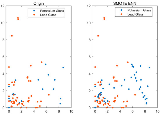
Figure 2.
Process Results.
2.2.3. Component Data
Component data refers to any non-negative n-vector and satisfies the constraint , which becomes a definite sum constraint and is the fundamental property of component data. It is clear from the context of this study that the data in the dataset are the composition percentages of each oxide in the glass artefact. Therefore all data in the dataset are compositional data. In order to better analyse the statistical laws of the data, this study has converted the valid data, and the conversion formula is shown in Equation (1), and the cumulative sum of the chemical composition of each group of data after conversion is 100%.
2.2.4. Centred Log-Ratio Transformation
The vector space in which the n-component data resides becomes a monomorphic space, and because monomorphic spaces are subject to fixed sum constraints, traditional statistical analysis methods for ordinary data are no longer applicable to component data. A review of the literature shows that analysis of monomorphic spaces often has the following three problems [31]:
- The intuitive form of the data differs between monomorphic and euclidean space and cannot be interpreted across space;
- The covariance matrices of the component data calculated on the monomorphic space are significantly biased negative, with very different connotations from those on the Euclidean space;
- The lack of parametric distribution of the component data on the monomorphic space makes it difficult to model the variational patterns of the data for analysis.
Based on the problems mentioned above, this study performs a centred log-ratio transformation (clr) on the data, which can more fully reflect the characteristics of the components after the central logarithmic ratio transformation and make the component data more interpretable. clr is calculated by the formula shown in Equations (2) and (3),
2.3. Methodology
As an essential part of artificial intelligence, computer science, and other fields, machine learning focuses on simulating human learning via the use of data, algorithms, and other techniques and steadily improving learning accuracy [32,33,34]. Machine learning is the process of acquiring knowledge through simulating data in order to predict or categorise new data. Currently, machine learning is widely used in pattern recognition issues such as image recognition [35,36,37], animal behaviour research [38] and classification.
According to the training approach, machine learning may be roughly divided into three categories: supervised learning, unsupervised learning, and reinforcement learning. Supervised learning is the application of supervised learning techniques when the target variables in the dataset are already known [39]. Unsupervised learning employs unsupervised learning methods when the initial dataset’s goal variables are unknown. Reinforcement learning is utilised to increase a model’s performance through repeated training.
It is possible to use supervised learning algorithms for regression analysis, classification research, and other domains. Support vector machines are a prevalent supervised learning method that may efficiently tackle binary classification issues. This study employs supervised machine learning to categorise the target variable, which is the kind of glass artefact. Because the target variable is binary and already known, supervised machine learning is used to classify the target variable.
2.4. Support Vector Machines
Support vector machines (SVMs) were introduced in 1964 and have developed rapidly since the 1990s with a series of improved and extended algorithms. The SVM learning approach is an advanced learning approach, the basic idea of which is the correct partitioning of the training dataset by mapping the boundary lines between classes and the categorisation that guarantees the maximum distance between the mapped boundary line classes, i.e., the separation of hyperplanes of separation, i.e., (Figure 3). SVM boundary lines are sometimes linear, sometimes using various kernel functions to predict more features, and for linearly divisible datasets, the hyperplanes have infinite numbers (i.e., perceptrons), but the longest geometrically spaced separated hyperplane is the only one.
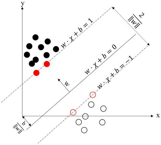
Figure 3.
Support vector machine principles.
SVM is widely used in pattern recognition problems, such as image recognition [40,41] and classification [42,43]. However, there are some drawbacks, such as the sensitive selection of parameters and kernel functions. It has been shown that the exact accuracy of model classification has been improved after genetic algorithms (GA) [44] and other algorithms have been introduced into SVM model optimisation. However, such optimisation algorithms suffer from the disadvantages of local optimality and difficulty in obtaining optimal parameters.
2.5. Slime Mould Algorithm
The slime mould algorithm (SMA) was proposed by Professors Li and Mirjalili in 2020 [45]. The algorithm simulates the behaviour of slime mould during the search for food, including movement, feeding, etc. During the optimisation process, the algorithm simulates the behaviour of a population of slime mould in the search for the optimal solution, changing the population distribution in the search space by simulating the reproduction and movement of slime mould and finally finding the optimal global solution. The slime mould algorithm has the advantages of fast convergence and strong global search capability and is well suited to complex optimisation problems, such as multi-dimensional, non-linear, and high-dimensional. Figure 4 illustrates the process of evaluating the fitness of slime mould in the foraging process. We can construct a model to describe the activity process of slime mould by the following mathematical formula.
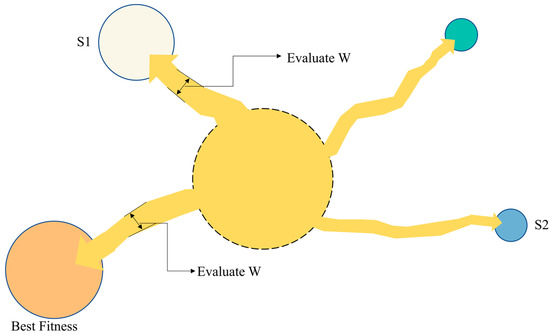
Figure 4.
Process adjusts to adaptability.
The approximate relationship between slime mould and food was modelled using a function with the following equation for positional updating.
In the equation, L and U are the upper and lower bounds of the search range, respectively, the parameters of take values in the range [−k, k], linearly decreases from 1 to 0, t is the current iteration, is the information of the location where the food odour concentration is found to be at the highest at the current r, X is the information of the current location of the slime mould, and are the randomly selected locations of the slime at A and B, W is the weight of the slime mould, j(i) is the fitness of X, and is the best fitness of all the best adaptation in all iterations.
The function expression for parameter k is
where is the maximum number of iterations. The expression for the mucilage weight is:
in Equation (9) represents the function that sorts the sequence, is the random value in the interval, is the best fitness obtained in the current iteration, represents the worst fitness obtained in the current iteration, and is the sequence of fitnesses.
2.6. Support Vector Machines Incorporating Slime Mould Algorithm Strategies
In recent years, the slime mould algorithm (SMA) has been successfully applied in a variety of fields as a novel optimisation algorithm [46,47]. In this study, we use the SMA to optimise the parameters of the SVM model. Before training the SVM model, the desirable range is determined by initialising the penalty factor C and the radial basis function parameter γ by using Equation (4). The solution is obtained as the optimal position obtained by the SMA. The optimal position is defined by the penalty factor C in the horizontal coordinate and the radial basis function parameter γ in the vertical coordinate. The resulting optimisation parameters C and γ are substituted into the support vector machine model for training.
2.7. Model Training
In machine learning, it is crucial to divide the dataset into a training set and a test set. The training set is used to train the model, while the test set is used to evaluate the performance of the model. The training set contains the data that the model needs to learn, while the test set contains data that the model has not seen before. This division helps to accurately assess the model’s ability to generalise to new data. In this study, 60% of the dataset was used for training, and 40% was used for testing.
In order to prevent overfitting and underfitting, it is important to pay attention to the performance of the model on both the training and test sets. Overfitting and underfitting are common problems in machine learning, where overfitting means that the model performs well on the training set but poorly on the test set. This is because the model is over-specialised in the training set, resulting in poor performance on new data. Underfitting, on the other hand, means that the model performs poorly on both the training and test sets. This is because the model has not learned enough features or does not have enough complexity to describe the data.
3. Results
3.1. Experimental Environment
The hardware environment used for the experiments in this paper: CPU: AMD Ryzen™ 7 4800H and 16 GB RAM, running on 64-bit Windows 11 operating system.
The experimental software environment Matlab 2022a was used for writing SVM for genetic algorithm optimisation and SVM for slime mould algorithm optimisation programs; SPSSPRO was used for SMOTE-ENN processing of the data and the construction of DT, RF, and SVM models. R was used for centred log-ratio transformation.
3.2. Experimental Results
3.2.1. Evaluation Indicators
This study used common evaluation metrics in classification tasks, such as training set accuracy, test set accuracy, precision, recall, and F1 score, to judge the model. Because the problem addressed in this study is a binary classification problem, a confusion matrix consisting of a four-unit window can be made. Figure 5 shows the confusion matrix for this study.
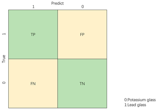
Figure 5.
Confusion Matrix. TP (True Positive): correct prediction for lead glass; TN (True Negative): correct prediction for potassium glass; FP (False Positive): incorrect prediction for lead glass; and FN (False Negative): incorrect prediction for potassium glass.
The accuracy is the proportion of correctly classified samples to the total number of samples combined with the confusion matrix, and the equation is calculated as in Equation (10).
Accuracy is the simplest and most intuitive metric to evaluate in classification problems, but it has obvious drawbacks. When experimenting, it is important to note that when the proportion of samples from different categories is very uneven, the category with the largest proportion tends to be the most significant factor affecting accuracy.
Precision refers to the proportion of the samples predicted to be positive by the model that is also actually positive as a proportion of those predicted to be positive. The calculation formula is Equation (11).
Precision provides a visual indication of the classifier’s ability to not mark negative samples as positive.
Recall refers to the proportion of samples that are actually positive that are predicted to be positive out of those that are actually positive. The calculation formula is Equation (12).
Recall visually illustrates the ability of the classifier to find all positive samples.
The F1 score is the summed average of Precision and Recall [48], calculated as
The F1 score can be interpreted as the weighted average of Precision and Recall. The F1 score is a combination of Precision and Recall. The higher the F1 score, the more robust the model is.
3.2.2. Results of the Optimisation Algorithm
In this study, we conducted an experimental study of two heuristic optimisation algorithms. To ensure the fairness of the experiments, we uniformly set the number of populations to 5 and set the range of values for the penalty factor C and the radial basis kernel function parameter γ to [0.01,100].
In the GA algorithm and SMA algorithm, fitness is an indicator to evaluate the strengths and weaknesses of an individual. During the iteration of the algorithm, the fitness value of an individual changes when the population evolves, resulting in a fitness curve. The fitness value is calculated as Equation (14).
The experimental results show that there is a significant difference in the fitness of the two algorithms. Figure 6 shows the fitness curves of the two algorithms during the experiments, and it can be found that the SMA algorithm has a faster adaptation speed than the GA algorithm.
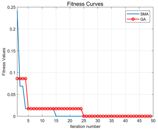
Figure 6.
Fitness Curve.
Combining the running times of the algorithms in Table 1, we can find that the SMA algorithm has a clear advantage in terms of computation time. Combining the results derived above, we can surmise that the SMA algorithm is a better choice while considering the computational efficiency.

Table 1.
Algorithm runtime.
3.2.3. Comparison of Classification Models
In this study, we compared multiple classification models. In order to represent the effectiveness of each model as much as possible, we did not use any pre-trained models but trained each model from scratch. We selected a variety of commonly used classification algorithms and used normalised parameter settings in our experiments to ensure fairness. We chose the parameters of the traditional machine learning algorithm considering the number of features of the data and the fact that the occurrence of overfitting should be avoided. The ggap in the GA algorithm indicates the survival ratio of the next generation and usually takes a value from 0.6 to 0.9. In this paper, the best experimental result is 0.7, which is chosen as the value of ggap. The selected parameters are shown in Table 2. The detailed results are shown in Table 3.
Table 2.
Selected parameters of each algorithm.
Table 3.
Results of model experiments.
4. Discussion
In this study, we parameterised the support vector machine using two heuristic optimisation algorithms and compared the results with classical machine learning models. The analysis of Table 1 shows that the SMA algorithm runs faster than the GA algorithm by 0.12959 s, which is a significant improvement of 45.7% in running time. According to the adaptation curve in Figure 6, we can deduce that the SMA algorithm has a faster number of iterations compared to the GA algorithm, which also verifies the improvement of algorithm speed from the side. The analysis of Table 3 reveals that the support vector machines optimised heuristically outperform the classical machine learning models in all metrics. Among them, the effect of the support vector machine optimised by GA and SMA is more than that of the classical support vector machine. After optimisation by the slime mould algorithm strategy, the test set accuracy is 5.0% higher than GA-SVM, the precision is 4.6% higher than GA-SVM, the recall is 4.6% higher than GA-SVM, and the F1 score is 4.5% higher than GA-SVM.
Taking into account the number of iterations of the algorithm, the running time and the excellence of the evaluation metrics, this study concludes that the model proposed in the paper is more suitable for this study and has the capability to carry out the work of identifying glass artefact types in the archaeological process. These results also show that the heuristic optimisation algorithm is an effective model optimisation method to improve the classification performance of support vector machines.
5. Conclusions
In this study, the slime mould algorithm is incorporated into the support vector machine model to improve the accuracy of the model and the efficiency of the system. The parameters of the support vector machine are optimally selected by the slime mould algorithm without changing the structure of the original algorithm. When training the model, indicators such as training set accuracy, test set accuracy, precision, recall, and F1 score are used to evaluate the model’s merit.
The experiments show that the model proposed in this paper performs well on the dataset and has a substantial improvement over all other classification models. In addition, the analysis of the running time and the number of iterations can be obtained that the SMA algorithm is fast and time-consuming in finding parameters, which helps to improve the system efficiency and save the running cost. In summary, this study concluded that the support vector machine model incorporating the slime mould algorithm strategy is a better choice for the classification of glass artefacts and gives more accurate classification results than before. The algorithm proposed in this study will be useful in revealing the potential trade relations and cultural exchanges between different regions in ancient times. Future researchers can adopt the algorithm proposed in this paper to classify ancient glass, which will be helpful in deeply exploring and inferring a more accurate and complete ancient trade network and cultural exchange pattern.
The dataset used in this study is based on the proportions of the chemical composition obtained from sampling points on the surface of the artefacts. It is clear that the main chemical composition of ancient glass artefacts from around the world is similar [49,50]. Therefore, the results obtained within the scope of this study can also be applied to glass artefacts excavated around the world for classification purposes. However, when applied to glass objects with significantly different compositional ratios, the results should be validated using a different methodology.
Future research directions for this study can be summarised as follows:
- The model will determine the classification of the newly excavated glass;
- The model can be compared with deep learning methods. It is limited by the small amount of data, and deep learning methods have not been utilised in this study;
- In conjunction with the location of the research samples and the distribution patterns of the material content of the local soils, the trade relationships between the ancient regions are determined.
Author Contributions
Conceptualisation, Y.G.; data curation, Y.G.; writing—original draft preparation, Y.G.; writing—review and editing, W.Z. and W.L.; supervision, W.Z.; project administration, W.Z.; funding acquisition, W.Z. All authors have read and agreed to the published version of the manuscript.
Funding
This research was funded by the National Natural Science Foundation of China, grant number 62276032.
Institutional Review Board Statement
This study did not require ethical approval.
Informed Consent Statement
Not applicable.
Data Availability Statement
Data are provided in the 2022 China Undergraduate Mathematical Contest in Modeling. The authors do not have permission to share the data.
Conflicts of Interest
The authors declare no conflict of interest.
References
- Lee, C.; Czae, M.-Z.; Kim, S.; Kang, H.T.; Lee, J.D. Classification of Korean ancient glass pieces by pattern recognition method. J. Korean Chem. Soc. 1992, 36, 113–124. [Google Scholar]
- Yoon, Y.Y.; Lee, K.Y.; Chung, K.S.; Yang, M.K.; Kim, K.H. Classification of Korean old potteries by trace elements analysis. J. Radioanal. Nucl. Chem. 2001, 248, 89–92. [Google Scholar] [CrossRef]
- Baert, K.; Meulebroeck, W.; Wouters, H.; Ceglia, A.; Nys, K.; Thienpont, H.; Terryn, H. Raman spectroscopy as a rapid screening method for ancient plain window glass. J. Raman Spectrosc. 2011, 42, 1055–1061. [Google Scholar] [CrossRef]
- Schibille, N.; Gratuze, B.; Ollivier, E.; Blondeau, É. Chronology of early Islamic glass compositions from Egypt. J. Archaeol. Sci. 2019, 104, 10–18. [Google Scholar] [CrossRef]
- Su, H.M. Characteristic Analysis of Chemical Compositions for Ancient Glasses Excavated from the Sarira Hole of Mireuksaji Stone Pagoda, Iksan. J. Conserv. Sci. 2017, 33, 215–223. [Google Scholar]
- Xingling, T.; Jianyu, W.; Yong, C. A study of glass beads recovered from the Ming Dynasty shipwreck of Nan’ao 1. Cult. Relics 2016, 12, 87–92. [Google Scholar] [CrossRef]
- Lin, Y.; Liu, T.; Toumazou, M.K.; Counts, D.B.; Kakoulli, I. Chemical analyses and production technology of archaeological glass from Athienou-Malloura, Cyprus. J. Archaeol. Sci. Rep. 2019, 23, 700–713. [Google Scholar] [CrossRef]
- Oikonomou, A.; Triantafyllidis, P. An archaeometric study of Archaic glass from Rhodes, Greece: Technological and provenance issues. J. Archaeol. Sci. Rep. 2018, 22, 493–505. [Google Scholar] [CrossRef]
- Wen, F.; Gui, G.; Gacanin, H.; Sari, H. Compressive sampling framework for 2D-DOA and polarization estimation in mmWave polarized massive MIMO systems. IEEE Trans. Wirel. Commun. 2022, 29, 2612–2616. [Google Scholar] [CrossRef]
- Wen, F.; Shi, J.; Gui, G.; Gacanin, H.; Dobre, O.A. 3-D Positioning Method for Anonymous UAV Based on Bistatic Polarized MIMO Radar. IEEE Internet Things J. 2022, 10, 815–827. [Google Scholar] [CrossRef]
- Xue, J.; Shen, B. Dung beetle optimizer: A new meta-heuristic algorithm for global optimization. J. Supercomput. 2022, 78, 1–32. [Google Scholar] [CrossRef]
- Narodytska, N.; Ignatiev, A.; Pereira, F.; Marques-Silva, J.; Ras, I. Learning Optimal Decision Trees with SAT. In Proceedings of the International Joint Conference on Artificial Intelligence, Stockholm, Sweden, 13–19 July 2018; pp. 1362–1368. [Google Scholar]
- Yang, Y.; Morillo, I.G.; Hospedales, T.M. Deep neural decision trees. arXiv 2018, arXiv:1806.06988. [Google Scholar]
- Iwendi, C.; Bashir, A.K.; Peshkar, A.; Sujatha, R.; Chatterjee, J.M.; Pasupuleti, S.; Mishra, R.; Pillai, S.; Jo, O. COVID-19 patient health prediction using boosted random forest algorithm. Front. Public Health 2020, 8, 357. [Google Scholar] [CrossRef] [PubMed]
- Gul, A.; Perperoglou, A.; Khan, Z.; Mahmoud, O.; Miftahuddin, M.; Adler, W.; Lausen, B. Ensemble of a subset of kNN classifiers. Adv. Data Anal. Classif. 2018, 12, 827–840. [Google Scholar] [CrossRef] [PubMed]
- Tang, H.; Xu, Y.; Lin, A.; Heidari, A.A.; Wang, M.; Chen, H.; Luo, Y.; Li, C. Predicting green consumption behaviors of students using efficient firefly grey wolf-assisted K-nearest neighbor classifiers. IEEE Access 2020, 8, 35546–35562. [Google Scholar] [CrossRef]
- Abhilash, P.; Chakradhar, D. Prediction and analysis of process failures by ANN classification during wire-EDM of Inconel 718. Adv. Manuf. 2020, 8, 519–536. [Google Scholar] [CrossRef]
- Zhang, Z.; Zhan, W.; He, Z.; Zou, Y. Application of spatio-temporal context and convolution neural network (CNN) in grooming behavior of Bactrocera minax (diptera: Trypetidae) detection and statistics. Insects 2020, 11, 565. [Google Scholar] [CrossRef]
- Assael, Y.; Sommerschield, T.; Shillingford, B.; Bordbar, M.; Pavlopoulos, J.; Chatzipanagiotou, M.; Androutsopoulos, I.; Prag, J.; de Freitas, N. Restoring and attributing ancient texts using deep neural networks. Nature 2022, 603, 280–283. [Google Scholar] [CrossRef]
- Hong, S.; Zhan, W.; Dong, T.; She, J.; Min, C.; Huang, H.; Sun, Y. A Recognition Method of Bactrocera minax (Diptera: Tephritidae) Grooming Behavior via a Multi-Object Tracking and Spatio-Temporal Feature Detection Model. J. Insect Behav. 2022, 35, 67–81. [Google Scholar] [CrossRef]
- Jiang, Y.; Xie, J.; Han, Z.; Liu, W.; Xi, S.; Huang, L.; Huang, W.; Lin, T.; Zhao, L.; Hu, Y. Immunomarker Support Vector Machine Classifier for Prediction of Gastric Cancer Survival and Adjuvant Chemotherapeutic BenefitImmunomarker SVM–Based Predictive Classifier. Clin. Cancer Res. 2018, 24, 5574–5584. [Google Scholar] [CrossRef]
- Ma, Z.; Dong, Y.; Liu, H.; Shao, X.; Wang, C. Forecast of non-equal interval track irregularity based on improved grey model and PSO-SVM. IEEE Access 2018, 6, 34812–34818. [Google Scholar] [CrossRef]
- Wang, S.-Y.; Bi, W.-H.; Gan, W.-Y.; Li, X.-Y.; Zhang, B.-J.; Fu, G.-W.; Jiang, T.-J. Identification of ichthyotoxic red tide algae based on three-dimensional fluorescence spectra and particle swarm optimization support vector machine. Spectrochim. Acta Part A Mol. Biomol. Spectrosc. 2022, 268, 120711. [Google Scholar] [CrossRef] [PubMed]
- Bin, S.; Jiancheng, W. Research advances in artificial intelligence for prognosis prediction of liver cancer patients. Acad. J. PLA Postgrad. Med. Sch. 2020, 41, 922–925, 953. [Google Scholar]
- Idrissi, B.Y.; Arjovsky, M.; Pezeshki, M.; Lopez-Paz, D. Simple data balancing achieves competitive worst-group-accuracy. In Proceedings of the Conference on Causal Learning and Reasoning, Eureka, CA, USA, 11–13 April 2022; pp. 336–351. [Google Scholar]
- Yi, H.; Jiang, Q.; Yan, X.; Wang, B. Imbalanced classification based on minority clustering synthetic minority oversampling technique with wind turbine fault detection application. IEEE Trans. Ind. Inform. 2020, 17, 5867–5875. [Google Scholar] [CrossRef]
- Wang, Z.; Cao, C.; Zhu, Y. Entropy and confidence-based undersampling boosting random forests for imbalanced problems. IEEE Trans. Neural Netw. Learn. Syst. 2020, 31, 5178–5191. [Google Scholar] [CrossRef]
- Puri, A.; Kumar Gupta, M. Improved hybrid bag-boost ensemble with K-means-SMOTE–ENN technique for handling noisy class imbalanced data. Comput. J. 2022, 65, 124–138. [Google Scholar] [CrossRef]
- Chawla, N.V.; Bowyer, K.W.; Hall, L.O.; Kegelmeyer, W.P. SMOTE: Synthetic minority over-sampling technique. J. Artif. Intell. Res. 2002, 16, 321–357. [Google Scholar] [CrossRef]
- Ishaq, A.; Sadiq, S.; Umer, M.; Ullah, S.; Mirjalili, S.; Rupapara, V.; Nappi, M. Improving the prediction of heart failure patients’ survival using SMOTE and effective data mining techniques. IEEE Access 2021, 9, 39707–39716. [Google Scholar] [CrossRef]
- Guo, L.; Guan, R. A Comparative Study of Compositional Data Transformation Methods Based on Spatial Equivalence. Stat. Appl. 2018, 7, 271. [Google Scholar]
- Zhan, W.; Hong, S.; Sun, Y.; Zhu, C. The system research and implementation for autorecognition of the ship draft via the UAV. Int. J. Antennas Propag. 2021, 2021, 4617242. [Google Scholar] [CrossRef]
- Chao, M.; Wei, Z.; Yuqi, Z.; Jianhua, L.; Shengbing, H.; Yu, T.T.; Jinhui, S.; Huazi, H. Trajectory tracking and behaviour of grain storage pests based on Hungarian algorithm and LSTM network. J. Chin. Cereals Oils Assoc. 1–13. Available online: http://kns.cnki.net/kcms/detail/11.2864.TS.20220708.1012.008.html (accessed on 20 February 2023).
- Mengyuan, X.; Wei, Z.; Lianyou, G.; Hu, L.; Peiwen, W.; Tao, H.; Weihao, L.; Yong, S. Maize leaf disease detection and identification based on ResNet model. Jiangsu Agric. Sci. 1–8. Available online: http://kns.cnki.net/kcms/detail/32.1214.S.20221107.0921.002.html (accessed on 20 February 2023).
- Zhan, W.; Zou, Y.; He, Z.; Zhang, Z. Key points tracking and grooming behavior recognition of Bactrocera minax (Diptera: Trypetidae) via DeepLabCut. Math. Probl. Eng. 2021, 2021, 1392362. [Google Scholar] [CrossRef]
- Sun, C.; Zhan, W.; She, J.; Zhang, Y. Object detection from the video taken by drone via convolutional neural networks. Math. Probl. Eng. 2020, 2020, 4013647. [Google Scholar] [CrossRef]
- Zhan, W.; Sun, C.; Wang, M.; She, J.; Zhang, Y.; Zhang, Z.; Sun, Y. An improved Yolov5 real-time detection method for small objects captured by UAV. Soft Comput. 2022, 26, 361–373. [Google Scholar] [CrossRef]
- She, J.; Zhan, W.; Hong, S.; Min, C.; Dong, T.; Huang, H.; He, Z. A method for automatic real-time detection and counting of fruit fly pests in orchards by trap bottles via convolutional neural network with attention mechanism added. Ecol. Inform. 2022, 70, 101690. [Google Scholar] [CrossRef]
- El Naqa, I.; Murphy, M.J. What is machine learning? In Machine Learning in Radiation Oncology; Springer: Berlin/Heidelberg, Germany, 2015; pp. 3–11. [Google Scholar]
- Huang, H.; Zhan, W.; Du, Z.; Hong, S.; Dong, T.; She, J.; Min, C. Pork primal cuts recognition method via computer vision. Meat Sci. 2022, 192, 108898. [Google Scholar] [CrossRef] [PubMed]
- Li, W.; Zhan, W.; Han, T.; Wang, P.; Liu, H.; Xiong, M.; Hong, S. Research and Application of U2-NetP Network Incorporating Coordinate Attention for Ship Draft Reading in Complex Situations. J. Signal Process. Syst. 2022, 94, 1–19. [Google Scholar] [CrossRef]
- Al-Dabagh, M.Z.N.; Alhabib, M.M.; Al-Mukhtar, F. Face recognition system based on kernel discriminant analysis, k-nearest neighbor and support vector machine. Int. J. Res. Eng. 2018, 5, 335–338. [Google Scholar] [CrossRef]
- Wang, R.; Li, Z.; Cao, J.; Chen, T.; Wang, L. Convolutional recurrent neural networks for text classification. In Proceedings of the 2019 International Joint Conference on Neural Networks (IJCNN), Budapest, Hungary, 14–19 July 2019; pp. 1–6. [Google Scholar]
- Li, X.; Kong, J. Application of GA–SVM method with parameter optimization for landslide development prediction. Nat. Hazards Earth Syst. Sci. 2014, 14, 525–533. [Google Scholar] [CrossRef]
- Li, S.; Chen, H.; Wang, M.; Heidari, A.A.; Mirjalili, S. Slime mould algorithm: A new method for stochastic optimization. Future Gener. Comput. Syst. 2020, 111, 300–323. [Google Scholar] [CrossRef]
- Kamboj, V.K.; Kumari, C.L.; Bath, S.K.; Prashar, D.; Rashid, M.; Alshamrani, S.S.; AlGhamdi, A.S. A cost-effective solution for non-convex economic load dispatch problems in power systems using slime mould algorithm. Sustainability 2022, 14, 2586. [Google Scholar] [CrossRef]
- Farhat, M.; Kamel, S.; Atallah, A.M.; Hassan, M.H.; Agwa, A.M. ESMA-OPF: Enhanced slime mould algorithm for solving optimal power flow problem. Sustainability 2022, 14, 2305. [Google Scholar] [CrossRef]
- Xiao, W.Y.; Yufen, T.; Li, Z.; Zhifei, X. A clinical prediction model for children with severe obstructive sleep apnoea. Chin. J. Pract. Pediatr. 2022, 37, 701–707. [Google Scholar] [CrossRef]
- Bugoi, R.; Mureşan, O. A brief study on the chemistry of some Roman glass finds from Apulum. Rom. Rep. Phys 2021, 73, 803. [Google Scholar]
- Bugoi, R.; Alexandrescu, C.-G.; Panaite, A. Chemical composition characterization of ancient glass finds from Troesmis—Turcoaia, Romania. Archaeol. Anthropol. Sci. 2018, 10, 571–586. [Google Scholar] [CrossRef]


Disclaimer/Publisher’s Note: The statements, opinions and data contained in all publications are solely those of the individual author(s) and contributor(s) and not of MDPI and/or the editor(s). MDPI and/or the editor(s) disclaim responsibility for any injury to people or property resulting from any ideas, methods, instructions or products referred to in the content. |
© 2023 by the authors. Licensee MDPI, Basel, Switzerland. This article is an open access article distributed under the terms and conditions of the Creative Commons Attribution (CC BY) license (https://creativecommons.org/licenses/by/4.0/).