Abstract
This research deals with a U-shaped assembly line balancing problem in which items are fixed on the conveyor. Operators execute the assembly tasks without removing items from the conveyor as the assembly items are assumed to be unsuitable for manual handling. The operators have to walk beside the conveyor at the same speed as the conveyor while they execute assembly tasks. If the operators want to assemble other items, they may have to walk to other positions at their normal walking speed. Therefore, the cycle time of an operator should include assembly times and walking times between assembly tasks. In this research, a mathematical model of the proposed U-shaped conveyor assembly line balancing problem was developed. Given a number of operators, the mathematical model can optimize the sequence of tasks and allocation of tasks to workstations using the commercial software LINGO 17. Because LINGO 17 requires a long computing time, simulated annealing (SA), which can accept worse new solutions in the search procedure, is proposed. The experimental results show that the proposed SA can optimize the problem efficiently.
1. Introduction
Conveyors are used when material is to be moved frequently between specific points [1]. When there is sufficient throughput between fixed points, the use of conveyors is suggested [2] for high-efficiency transport over short and medium distances [3,4]. Conveyors are also used in assembly line systems, generally in two different configurations. In the first, items are transported between machines by conveyors. Once the items arrive at a machine, the operators move them off the conveyor for assembling and then put them back on the conveyor to move them to subsequent machines. In this case, the positions of operators are fixed when assembling items. In the second case, the items may be large or not easily handled, and are not easily moved. The items are fixed to the moving conveyor, and operators execute their assembly tasks moving beside the conveyor as they work. After finishing all their assembly tasks, the operators walk back to their original locations and execute the assembly tasks for the next item. The present study aims to solve an assembly line balancing problem in which the conveyor belongs to the second case.
Line balancing involves allocating an equal amount of work to each workstation along the line [5]. The fundamental line balancing problem is to assign a set of tasks to an ordered set of workstations, so that the precedence relationships are satisfied and some measure of performance is optimized [6]. For the second case of conveyor assembly lines, operators have to move along the conveyors while executing assembly tasks and walk back to their original locations after finishing the assembly tasks assigned to them. Walking time between assembly tasks should be taken into consideration when balancing such assembly lines.
In traditional straight assembly lines, the walking times are proportional to the corresponding assembly times and can be integrated into assembly time, because the operators walk back to their original locations beside the conveyor and the times depend on the distance that the conveyor moves while the operators execute the assembly tasks. A U-shaped conveyor assembly line, however, is divided into two sub-lines: the entrance sub-line and exit sub-line. An operator may be able to execute assembly tasks on both sub-lines within the same work cycle [7], and the estimation of walking times between assembly tasks for each operator is more complicated. For example, in Figure 1, there are 7 assembly tasks. The assembly sequence is 1, 2, 3, 4, 5, 6, and 7, so that no precedence relationships are violated. Tasks 1 and 7 are assigned to Operator 1, Tasks 2 and 6 are assigned to Operator 2, and Tasks 3, 4 and 5 are assigned to Operator 3. According to the sequence and the corresponding assembly times, a, b, c, d, e, f, g, h indicate the starting and completing points of tasks. The dotted lines with arrows are the walking paths between assembly tasks. For example, Operator 1, executes assembly Task 1 from point a to point b, taking the assembly time of Task 1, and then walks to point g without executing assembly tasks. He/she then executes assembly Task 7 from point g to point h, taking the time of Task 7, and then walks back to point a without executing assembly tasks.
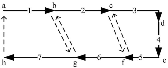
Figure 1.
An example of walking paths in a U-shaped conveyor assembly line.
According to the example shown in Figure 1, the time spent walking between assembly tasks depends on the sequence of tasks, the assembly time of tasks, the allocation of tasks to workstations and the configuration of the U-shaped conveyor assembly line. Therefore, it is not easy to take walking times into consideration when balancing the second case of U-shaped conveyor assembly lines where the items are fixed to the conveyor.
There are four types of assembly line balancing problem [8]. Type 1 aims to minimize the number of stations for a given cycle time. Type 2 aims to minimize the cycle time for a given number of workstations. Type E aims to maximize the efficiency with a specified cycle time or number of workstations. Additionally, Type F aims to find a feasible design for a given cycle time and number of workstations. This research deals with a problem of Type 2, which is encountered frequently when the production rhythm must be adjusted to the manufacturing process [7].
This research deals with the problem of balancing the second case of U-shaped conveyor assembly line. Two decisions must be made to minimize the cycle time for a given number of operators: (1) the sequence of assembly tasks along the conveyor line and (2) the allocation of sequences (corresponding tasks) to workstations (operators). The walking times between assembly tasks are included in cycle times. A mixed-integer programming model that can be optimized using LINGO 17 is developed. LINGO is a comprehensive tool designed to make building and solving mathematical optimization models easier and more efficient [9]. It utilizes the power of linear and non-linear optimization to formulate large problems concisely and solve them [10]. In order to optimize the U-shaped conveyor assembly line efficiently, a simulated annealing (SA) is proposed. Some problems that have been studied in [11,12,13,14,15,16,17,18] are modified for testing.
2. Literature Review
Research that deals with problems that relate to balancing conveyor assembly lines mainly focuses on traditional straight assembly lines. Xiaobo and Ohno [19] dealt with the concept in the Toyota production system, which permits operators to stop the conveyor whenever they fail to complete the operations within their work stations in a mixed-model assembly line. They took walking time into consideration to formulate a sequencing problem and then proposed a heuristic algorithm to minimize total conveyor stoppage time. Zhao et al. [20] described a balancing problem for mixed-model assembly lines with a paced moving conveyor. All operators can only execute their assembly tasks within a boundary. Operators execute their assembly tasks as the items move on the conveyor, then walk back to the position of the next product that the assembly tasks assign to them. If assembly tasks cannot be completed within the boundary, overload time occurs. When overloads occur, the unfinished assembly task has to be completed offline or the conveyor must be stopped temporarily. A heuristic is proposed to minimize the total overload time. Mendes et al. [21] described a mixed-model PC camera assembly line balancing problem. Firstly, a heuristic procedure previously developed based on the SA meta-heuristic, is used to derive line configurations with a minimum number of workstations and a smooth workload balance between and within the workstations. Then, the solutions provided by the heuristic procedure are used as an input to discrete event simulation models in order to test the robustness of these solutions. Kim and Jeong [22] proposed a heuristic procedure for optimizing the input sequence of product models with sequence-dependent setup times in a mixed-model assembly line using a conveyor system. All operators are forced to complete their operations within their predetermined work zone. The goal is to minimize the total of unfinished work within their work zone. Experimental results show that the heuristic procedure provides reasonably good solutions with low computational costs. Kim et al. [18] presented a mixed-integer programming model and a genetic algorithm (GA) to solve the minimum cycle time with a given number of workstations for two-sided assembly line balancing problems in which different assembly tasks on the same product item can be performed in parallel on both sides of the conveyor line. The experimental results show that the proposed GA outperforms the heuristic and the existing GA. Defersha and Mohebalizadehgashti [23] proposed a mixed-integer linear programming mathematical model to optimize balancing and sequencing problems for a continuously moving conveyor. They developed a multi-phased linear programming embedded GA to minimize the length and number of workstations, costs of workstations and task duplication. Numerical examples were presented to illustrate the model and the computational efficiency of the developed hybrid genetic algorithm. Based on the results obtained, the proposed algorithm outperformed the branch and bound algorithm in finding acceptable solutions. Pearce et al. [24] presented a complex line balancing problem based on a real conveyor assembly environment with task-to-task relationships, station characteristics limiting assignment, and parallel worker zoning interactions. A heuristic, combining rank-position-weighting, last-fit-improvement and iterative blocking schemes, and an integer programming that can manage multiple constraint types simultaneously were developed. Experimental results indicate that the integer programming model provides a viable solution method for those industries with access to commercial solvers.
Research dealing with U-shaped conveyor assembly line balancing problems is rare. Hwang et al. [25] proposed a multi-objective genetic algorithm to solve the U-shaped conveyor assembly line balancing problem. The performance criteria considered were the number of workstations (equal to the number of operators) and the variation of workload. Hwang and Katayama [11] proposed a new evolutionary approach to deal with workload balancing problems in mixed-model U-shaped conveyor assembly lines. The same task on different products is assumed to take the same time. The performance criteria were the same as Hwang et al. [25]. A case study was examined as a validity check in collaboration with a manufacturing company. Li et al. [26] dealt with U-shaped conveyor assembly line balancing problems in which task times are uncertain and corresponding historical information is not available due to technology changes, environmental changes, or the effect of learning on the part of operators. An uncertain programming model that minimizes the number of workstations was proposed first. Then, the uncertain model was transferred into a deterministic model to reduce computational effort. Finally, an algorithm was developed based on a branch and bound memory algorithm to find the optimal solution. Although Hwang et al. [25], Hwang et al. [11] and Li et al. [26] dealt with U-shaped conveyor assembly line balancing problems, they ignored walking times.
U-shaped assembly line balancing problems are similar to the proposed problem, but most of them also ignored walking times. In recent years, Zhang et al. [27] addressed the Type 2 U-shaped robotic assembly line balancing problem, in which the objectives are to minimize the cycle time and energy consumption simultaneously. The Pareto artificial bee colony algorithm (PABC) is extended to tackle this problem. Zhang et al. [28] applied an occupational repetitive action method to calculate the ergonomic risk value. A worker assignment and balancing problem of Type 2 for a U-shaped assembly line to minimize cycle time and ergonomic risks was then formulated. A multi-objective restarted iterative Pareto greedy algorithm is proposed to tackle this problem. Chantarasamai and Lasunon [29] described a differential evolution algorithm for solving U-shaped assembly line balancing problems. The objective is to minimize cycle time for a just-in-time production line that produces a single product with a certain number of workstations. Pinarbasi [30] considered a U-shaped assembly line balancing problem with stochastic assembly times. Two new chance-constrained non-linear models are proposed. The results are compared with the results of modified ant colony optimization and a piecewise-linear programming model. The study shows that the proposed two models are more effective and successful in solving stochastic U-shaped assembly line balancing problems. Chutima and Khotsaenlee [31] dealt with the parallel adjacent U-shaped assembly line balancing problem. Operators and robots are assigned to execute assembly tasks in the same work cycle. Assembly tasks located in two adjacent U-shaped assembly lines can assigned to the same operator or robot. Moreover, both fully able and disabled operators are considered. A mathematical model with five objective functions is developed. Then, non-dominated sorting teaching-learning-based optimization is proposed to solve the proposed problems. Khorram et al. [32] aim to optimize activity-to-station and operator-to-station decisions in a U-shaped assembly line balancing problem. Criteria such as equipment cost, number of stations and quality of activity performance are considered simultaneously. As an approach to solving the problem, classical simulated annealing (SA), variable neighborhood search (VNS), and a genetic algorithm (GA) were adopted for optimization.
Very few studies consider walking times in U-shaped assembly line balancing problems. Ohno and Nakade [33] considered walking times and formulated the optimal operator allocation problem to minimize the overall cycle time and discussed the two operator allocation problem as a special case. Nakade and Ohno [34] proposed an algorithm for finding an optimal allocation of operators to machines that minimizes the cycle time for the minimum number of operators. Shewchuk [35] proposed a mathematical model that takes walking time into account, with operators following circular paths and walking around other operators. A heuristic algorithm was developed to optimize the allocation of operators. Although Ohno and Nakade [33], Nakade and Ohno [34] and Shewchuk [35] take walking times into consideration, the sequence of tasks is fixed and unchangeable. Kuo et al. [36] proposed an integer programming formulation which takes both precedence relationships of tasks and walking times between locations into consideration. The sequence of tasks and allocation of operators are optimized simultaneously. The four studies that consider walking times, described above, assume that the locations of items are fixed, and a conveyor is not used to move the assembled products. If operators have to execute another consecutive assembly task, they have to walk to the next location. However, as shown in the example illustrated in Figure 1, the present study aims to deal with a U-shaped conveyor assembly line balancing problem in which items are moved on when assembled. When operators have to execute another consecutive assembly task, they are already located at the start point of the next assembly task, and no additional walking is required.
This research aims to optimize a Type 2 U-shaped conveyor assembly line balancing problem with walking time between assembly tasks. Although very few research studies deal with walking times, such studies assume that items are assembled in fixed locations. Therefore, the problem that the present study addresses cannot be found in the literature. Since walking time is an important component of the cycle time, the present study is novel and contributes to the related literature on industrial processes. Based on the proposed problem, this research proposes integer programming to minimize cycle times with a given number of operators. An SA algorithm is also proposed to solve the problem efficiently. The resulting process may be of benefit in many related industries.
3. Integer Programming
In order to solve the proposed task sequencing and task allocation problems to balance the Type 2 case of U-shaped conveyor assembly lines, a mixed-integer programming model is developed. The main purpose of the proposed model is to minimize the cycle time. The sequence of all tasks must follow the precedence relationships of assembly. Therefore, a corresponding sequence number is assigned to each task. For each workstation, a single operator is assigned to execute all tasks that are allocated in it. The walking times between assembly tasks are taken into consideration. For two consecutive tasks in the same workstation, the second task starts where the first task ends. In this case, the walking times are zero and can be ignored. A mathematical programming model is proposed, for which the following notation is used:
Indices
i, r, s: task index,
j, p, q: sequence number index,
w: workstation index, and
e: segment index.
Parameters
I: number of tasks.
J: sequence number of last task in the task sequence.
: number of workstations (equal to number of operators available).
: a precedence relationship between tasks; if means assembly task r must be completed before task s starts.
: cycle time.
: walking time from assembly task with sequence number p to q.
: normal velocity of working.
: velocity of conveyor (smaller than VW).
: the length of the U-shaped conveyor assembly cell.
: the width of the U-shaped conveyor assembly cell.
: assembly time of task i.
: X coordinate of completing point of assembly task with sequence number j.
: Y coordinate of completing point of assembly task with sequence number j.
: moving distance of an item from the entrance point of the U-shaped conveyor to the completing point of assembly task with sequence number j.
Decision variable
Minimize CT
The model aims to minimize the cycle time as given in Equation (1). The cycle time is the maximum cycle time of all workstations, which will be as presented in Equation (22). Equation (2) ensures that only one sequence number is assigned to each task and Equation (3) ensures that each sequence number is only assigned once. Based on Equations (2) and (3), Equation (4) ensures that each task is assigned to only one workstation. Equation (5) represents the relationship between length, width and conveyor moving velocity as shown in Figure 2. Equation (6) is used for calculating the moving distance from the entrance point of the U-shaped conveyor assembly line to the point where the assembly task with corresponding sequence number is completed. In this research, the U-shaped assembly line is divided into three segments—the entrance segment, the U-turn segment and the exit segment—as shown in Figure 2. Equation (7) ensures that the completion point of each task is located in only one segment, and Equations (8)–(10) determine the segment in which the completion point of the task with the corresponding sequence number is located.
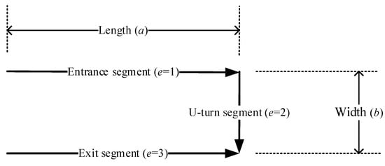
Figure 2.
Length, width and three segments in a U-shaped conveyor assembly line.
Equations (11) and (12) are used to calculate the coordinates of the completion point of each task with the corresponding sequence number. The exit point of the conveyor is set as (0, 0) and the entrance point is set as (0, b). If task r has to be completed before task s starts, based on the assembly sequence, Equation (13) avoids assembly task r being assigned to the larger sequence number than assembly task s. For two tasks with sequence numbers p and q which are not consecutive and are assigned to a single operator, when the operator completes the assembly task with sequence number p, he/she is at the completion point of the task, and he/she has to walk to the start point of the assembly task with sequence number q to execute the assembly task. Equation (14) is used to calculate the walking time from the completion point of an assembly task with sequence number p to the starting point of an assembly task with sequence number q.
When operators execute assembly tasks, they move at the velocity of the conveyor. Thus the moving times are equal to assembly times of the corresponding assembly tasks. However, when operators walk between assembly tasks, they walk at their normal walking speed. This research modifies the formulation proposed by Kuo et al. [36] to consider this issue. Equations (15)–(20) determine the walking paths between assembly tasks for operators in their corresponding workstations. When an operator completes all the tasks that are allocated to their workstation, they have to walk back to the first task of the workstation. Equations (15)–(17) determine the return walking path between tasks with sequence numbers and , when . Equation (15) determines the path when and . Equation (16) determines the path when and . Equation (17) determines the path when and . Equations (18)–(20) determine the walking path that relates to tasks with sequence numbers 1 and J. Equation (18) determines the path when and . Equation (19) determines the path when and . Equation (20) determines the path when and .
Equation (21) determines the walking path between non-adjacent locations and , when . If a walking path is determined by Equation (21), that indicates that the workstation is a crossover workstation. Figure 3 illustrates examples of paths that are determined by Equations (15)–(21). The total assembly time and walking time between assembly tasks in a workstation is the cycle time of the workstation and cannot exceed the cycle time of the U-shaped conveyor assembly line given in Equation (22).
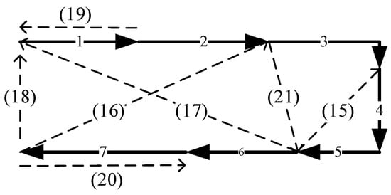
Figure 3.
Examples for Equations (15)–(21).
4. Proposed Methodology
In this research, an SA algorithm is developed to optimize the task sequencing and task allocation for the proposed U-shaped conveyor assembly line balancing problem. Kirkpatrick et al. [37] first proposed SA for optimization problems. It is a technique based on ideas from statistical mechanics and is based on the analogy with the behavior of a physical annealing processes in solids [38]. The SA algorithm has been widely used in solving sophisticated optimization problems [39]. SA uses a stochastic approach to search for new solutions, Snew, from the current Solution, S. If a better solution is found, the new solution will be accepted and the current solution will then be replaced. Based on the accepted solution, it continues to search for new solutions [40]. In order to escape from a local optimum, SA gives an opportunity to accept a new solution based on the probability . Z(Snew) and Z(S) are the performance of the solution Snew and S. It follows that the greater the difference in performance between Z(Snew) and Z(S), the smaller is the probability that the new solution will be accepted. E is called the “temperature”, and gradually reduces, or cools. Thus, in the search process, the probability of accepting a worse solution to escape a local optimum decreases.
In order to use SA to solve the U-shaped conveyor assembly line balancing problem, the operation of initial solution generation, performance evaluation, search for new solutions and temperature cooling should all be specified. The details are given below.
4.1. Initial Solution
This research proposes a two-phase procedure to generate initial solutions. The first is task sequencing and the second is task allocation. In the task sequencing phase, based on the precedence relationships between pairs of tasks, all tasks are sequenced. This means sequence numbers are assigned to tasks. The procedure is as follows:
Step 0: Set j = 1, C = set of tasks without any immediate precedence task.
Step 1: Select a task i form C at random and let Xij = 1.
Step 2: If j = J, then stop. Otherwise, delete task i from C and add tasks whose immediate precedence task is i into C.
Step 3: Let j = j + 1 and go to step 1.
In Figure 4, for example, the matrix shows that there are eight tasks and nine precedence relationships. Each “1” indicates one precedence relationship. The “1” in the first row and second column indicates that Task 2 can be started only if Task 1 is completed. The numbers under the matrix are the numbers of immediate precedence tasks of each task. Only Task 1 has no immediate precedence task. Therefore, in the beginning C = {1}. After sequence number 1 is assigned to Task 1, Tasks 2 and 3 will be added to C and Task 1 will be deleted from C. Therefore, C = {2, 3} and Task 2 and Task 3 can be randomly selected. Then, sequence number 2 will be assigned to the selected task. The procedure finally stops when all tasks are selected and sequence numbers are assigned. All tasks can be sequenced by the sequence numbers that are assigned to them. Figure 5 shows an example result.
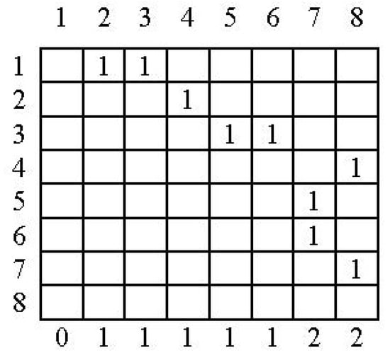
Figure 4.
An example matrix of precedence relationships.
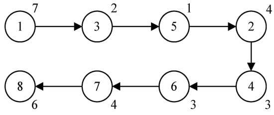
Figure 5.
An example result of task sequencing.
Based on the task sequence generated in the first phase, the second phase allocates tasks to workstations based on the sequence number assigned to them. The tasks whose locations are closer to the entrance or exit of the U-shaped conveyor assembly line are more likely to be allocated to the far left workstations. The task with sequence numbers 1 and J (the last task in the sequence) has the highest priority to be assigned to the first workstation. Assume that D is the set of two sequence numbers that can be assigned to a workstation, the procedure of the second phase is designed as follows:
Step 0: Calculate average cycle time , and let
Step 1: Set w = 1, D = {, } = {1, J}and all Yjw = 0.
Step 2: Randomly select a sequence number from D, and Let Yjw = 1.
Step 3: If sequence number was selected then = + 1, otherwise = − 1.
Step 4: If = , let and go to step 7. Otherwise, go to step 5.
Step 5: If , let w = w + 1. Otherwise, go to step 2.
Step 6: If w = Wmax, let for , …, and go to step 7. Otherwise, go to step 2.
Step 7: If , then stop. Otherwise go to step 8.
Step 8: and go to step 1.
In Figure 4, for example, the number beside each cycle is the assembly time. If Wmax = 3, then the average total assembly time (AC) and is 10. First, D = {1, 8}. If the task with sequence number 1 is assigned to Workstation 1, then tasks with sequence numbers 2 and 8 will be the candidate sequence numbers to be selected to be assigned to Workstation 1, as 7 < 10. If the task with Sequence number 8 is selected, then D = {2, 7} will be the candidate sequence numbers for Workstation 2, as 7 + 6 > 10. The procedure finally stops when = and the sequence number is assigned to the last workstation. Figure 6a shows an example initial result.
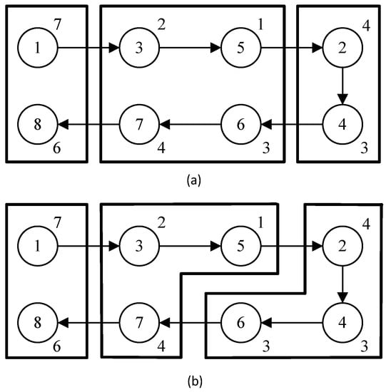
Figure 6.
An example result of task allocation, (a) original; (b) final.
In Step 5, one task can be assigned to the next workstation only when the total assembly time is more than the average total assembly time. Therefore, when the procedure assigns tasks to the last few workstations, it is possible that no task can be assigned. This situation can happen especially for cases with a large number of workstations. Thus a very unbalanced initial solution may be generated. Therefore, in Step 7, the cycle time of the last workstation is checked. If the cycle time of the last workstation is smaller than , AC will be reduced by Step 8 in which is a positive number smaller than 1. Then, a new solution will be generated. In Figure 6a, the cycle time of Workstation 3 is smaller than 10. Therefore, the procedure tries to generate new solutions until the cycle time of Workstation 3 is more than 10. Figure 6b shows an example final result.
4.2. Performance Evaluation
In the proposed integer programming model, the main solutions are represented by Xij and Yjw. In Figure 6, the assignment of sequence numbers to tasks and the allocation of tasks to workstation are represented. However, the real locations (including start and completion points) of tasks depend on the sequences and assembly times of tasks. Figure 7 illustrates the real locations of all tasks for the example in Figure 6. The arrangement also effects the walking distances between assembly tasks of all operators, as shown by dotted lines with arrows in Figure 7. Based on the proposed mathematical model, the time of each solution can be generated by the following steps.
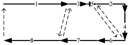
Figure 7.
Real locations of all tasks for the example in Figure 5.
Step 0: Given Xij, Yjw, a, b, VW and Ti.
Step 1: Calculate all walking times, WTpq, by Equations (6)–(14).
Step 2: Decide the paths that operators walk between assembly tasks, Upqw, by Equations (15)–(21).
Step 3: Calculate the cycle of each workstation by the left hand side of Equation (22).
Step 4: Return the longest cycle time among all workstations.
4.3. Searching for New Solutions
The proposed SA searches for new solutions by moving a sequence of tasks to another workstation. In order to search for a better solution, two constraints should be observed. First, sequences allocated to a workstation with a longer cycle time should be more likely to be selected to be reallocated to the adjacent workstation. Second, there must be no interference between operators in the new solution. The procedure for searching new solutions is as follows:
Step 0: Set Aw for w = 1~. (Aw is the set of sequence numbers whose corresponding tasks are assigned to workstation w).
Step 1: Select a workstation w at random, based on the probability .
Step 2: If only one task is assigned to workstation w (=1), go to step 1. Otherwise go to step 3.
Step 3: Select a sequence number j at random from .
Step 4: If , go to step 3. Otherwise go to step 5.
Step 5: Calculate , the workstation that task with sequence number j is assigned to ( for j = 1~J, and ).
Step 6: Randomly select another workstation among to , and let and .
For example, if Figure 6a is the current solution, and all Yjw can be represented by the matrix in Figure 8, the set Aw are in the right hand side of the matrix, and Bj are shown in the bottom of the matrix. Initially, the probability of workstations being selected to have one task removed are (13/30, 10/30, 7/30). Assume that Workstation 2 is selected and then task with sequence number 6 selected. As Y52 = 0, and B5 = 3, B7 = 2, then the task with sequence number 6 can be moved to either Workstation 3 or Workstation 2. However, the task with sequence number 6 was originally assigned to Workstation 2, so it will be moved to Workstation 3. The result is shown in Figure 9. The purpose of Step 6 is to comply with the second constraint. In the example, if the task with sequence number 6 is assigned to Workstation 1, interference occurs between operators in Workstations 1 and 2, as shown in Figure 10.
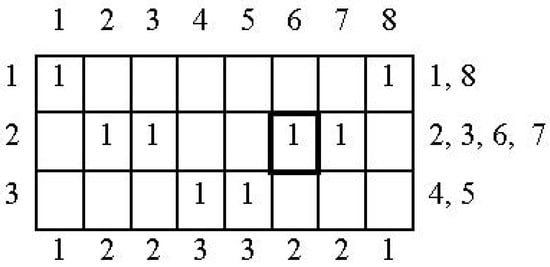
Figure 8.
An example for set Aw and Bj calculation.
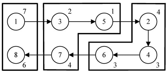
Figure 9.
An example result of a new solution.
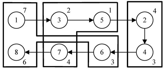
Figure 10.
An example result of a new solution with interference.
In Step 4, the purpose is to prevent the selection of a task that cannot be allocated to another workstation. If the task with sequence number j is selected, but both sequence number j − 1 and j + 1 are allocated in the same workstation. , and are the same, and no other workstations can be selected in Step 6.
4.4. Temperature Cooling
Temperature is an important parameter for accepting a worse solution in order to escape from a local optimum. This study adopts the cooling function which was introduced by Lundy and Mees [41] as shown in Equation (23). In Equation (23), Eh is the temperature in search iteration h, H is the total number of search iterations of SA, and β is the parameter for controlling the cooling speed. Lee et al. [39] mentioned that the cooling function outperforms the commonly used geometric temperature updating scheme.
The temperature given by Equation (23) is strictly decreasing. The proposed SA algorithm searches for new solutions based on the same task sequence and would settle on a local optimum. This research generates a new “initial solution” if no better solution is found after F search iterations in the SA procedure.
The total proposed SA procedure is illustrated in Figure 11.
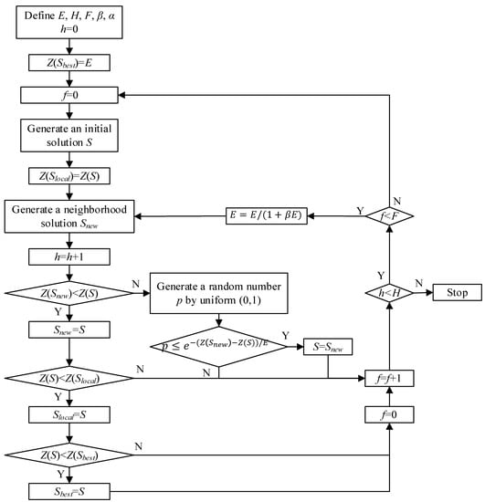
Figure 11.
Proposed SA procedure.
5. Experimental Results
In this research, 10 small problems were firstly collected from the literature. The corresponding information about the problems is summarized in Table 1. For each problem, the velocities of walking and conveyor (VW and VC) are assumed to be 4 and 1 per time unit. So the length of the conveyor is equal to the total processing time. In addition, the widths of the U-shaped conveyors (b) are set as 10% and 15% of the length of the conveyor, respectively. The proposed integer programming was tested using software LINGO 17 with 6 h maximum computing time. The results of two, three and four workstations are shown in columns 2, 5 and 8 in Table 2 and Table 3.

Table 1.
Summary of small problems.
Table 2.
The cycle times of experimental results for small problems (b = 10% of length of the conveyor).
Table 3.
The cycle times of experimental results for small problems (b = 15% of length of the conveyor).
As for the SA, it is assumed that total processing time () is probably the cycle time of the worst case in which all tasks are assigned to same workstation, and AC () is the cycle time of the best case. This means would be the upper bound of difference in performance between Z(Snew) and Z(S). This research set the initial temperature E as the total processing time. This means when there are two workstations, the acceptance probability for the initial temperature will be , which is greater than 60%. The minimum acceptance probability for the initial temperature will reduce as the number of workstations increases. However, the reduction is small. For example, when there are 20 workstations, the acceptance probability for the initial temperature will be , which is greater than 38%.
For the remaining SA parameters, F, H, α and β, a full factorial experiment is adopted based on Problem 10 with b = 10% and 4 workstations. For the four parameters, two levels are designed as shown in Table 4.
Table 4.
The design factors for SA parameters.
According to the experimental results, the main effect of all factor levels are illustrated in Figure 12. The smaller the cycle time the better. Therefore, F, H, α and β are set as , , 0.1 and 0.005, respectively. Moreover, the used for generating initial solutions is set as 0.1.
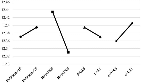
Figure 12.
The main effect of cycle time.
Based on the setting of parameters, the results of the proposed SA are shown in column 3, 6 and 9 in Table 2 and Table 3. It is found that the proposed SA results in a higher cycle time in 6 cases out of 60. This research then checked the six results generated by LINGO 17 in detail, and interference was found in Problem 3 with three workstations for both b = 10% and b = 15%. Interference always affects the performance of operators, and it can be avoided by the proposed SA. The detail of this operation is introduced in Section 4.3. Therefore, the performance difference between LINGO 17 and the proposed SA is almost the same if Problem 3 with three workstations for both b = 10% and b = 15% are excluded.
Moreover, the computation time of the proposed SA is strongly related to the number of iterations which is based on the number of tasks (). Using a computer with Intel Core i7-9700 3.00 GHz for Problems 1 to 3, the average computation time is 214 s. For Problems 4 to 7, the average computation time is 249 s. For Problems 8 and 9, the average computation time is 264 s. Additionally, for Problem 10, the computation time is 301 s. As regards LINGO 17, the computation times for 60 cases are shown in Figure 13.
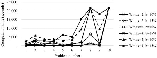
Figure 13.
Computation time of LINGO 17.
In Figure 13, the computation times required by LINGO 17 are case by case. In general, it is found that more computing time is required when there are more tasks or workstations. When there are 10 tasks (Problem 10), the computation times for all cases are 21,600 s (6 h). This means that more computation time would be required if a maximum computation time was not set.
Six larger problems were also collected from the literature. The original objectives of these problems are not the same as in the present study. The collected problems are modified for testing the performance of the proposed SA. The corresponding information is summarized in Table 5.
Table 5.
Summary of larger problems.
For the six problems in Table 5, b = 10% was tested. Due to the complexity of the proposed mathematical model, generating appropriate solutions for larger problems in reasonable computation time may be difficult using LINGO 17. In order to show the performance of the proposed SA, this research tried to analysis the performance of the results by their corresponding efficiency, which can be calculated by Equation (24).
In Equation (24), indicates the cycle time of workstation w. It can be calculated by the left hand side of Equation (22). The efficiency of the results of all cases are illustrated by line chart in Figure 14. All six problems are indicated by two numbers. The first of which is the problem number and the second, in parentheses, is the number of workstations.
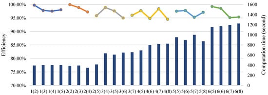
Figure 14.
The efficiency of the results of larger problems.
As shown in Figure 14, the efficiency is the lowest for Problem 4 with eight workstations and the corresponding efficiency is 94.53%. This means the proposed SA provided a relatively high quality, balanced design for a U-shaped conveyor assembly line. The computation times for all cases are also illustrated in Figure 14 by the bar chart. Because the total number of search iterations of SA is set as , more computation time is required by the problems with more tasks. The maximum computation time is found for Problem 6 when the number of workstations is eight. In that case, the computation time is 1222 s. This means the solutions can be provided in approximately 20 min when the number of tasks is 40. This indicates that the proposed SA is efficient and effective in solving practical problems. For cases with more workstations or tasks, it will be more efficient to use the proposed SA to optimize the problem.
6. Conclusions
This research dealt with a U-shaped assembly line balancing problem, in which the assembled items are fixed on the conveyor. Operators have to follow the conveyor while executing the assembly tasks assigned to them. After completing the assembly jobs on one item, the operators then walk to another point to execute the assembly jobs on other items. Therefore, both assembly times and walking times are included in the cycle time.
For the proposed U-shaped assembly line balancing problem, a mixed-integer programming model was first developed. The developed model can be optimized by commercial software LINGO 17. However, the computation time increases rapidly when the number of tasks and workstations increases. Simulated annealing (SA) was then proposed for optimizing the proposed U-shaped assembly line balancing problem. As there are many parameters in the proposed SA algorithm, a full factor experiment was adopted to find the optimal parameters setting. According to the experimental results from small problems, the proposed SA and LINGO 17 find similar solutions, but the computing times required by the proposed SA are much shorter. In order to show the efficiency of the proposed methodology, six larger problems are also tested. The results show that the efficiency of all problems is higher than 94%. Moreover, the computation times are approximately 20 min when the number of tasks is 40. Therefore, the proposed SA is also efficient for problems with more tasks or workstations.
Moreover, some research deals with assembly line balancing problems with stochastic assembly times. Although the variance in assembly time can be reduced and ignored when operators receive enough training for specific assembly tasks, the assembly times may vary even for well-trained operators and should be considered when optimizing the assignment of tasks to workstations. Moreover, interference between operators always reduces performance and should be avoided in any production line if possible. Checking all the results that were optimized by LINGO 17, interference was found in one case. This means that avoiding interference is not taken into account by the proposed mixed-integer programming model. Adding the influence of interference between operators into the proposed model and SA procedure could make it more applicable to real cases. This could suggest a future direction for work based on the present study.
In addition, in the proposed SA, only one strategy was proposed for searching for new solutions. Adopting various strategies for searching for new solutions may enrich the search directions and increase the chances of finding better solutions. Developing more search strategies for the proposed SA algorithm could also be an opportunity for future research.
Author Contributions
Conceptualization, Y.K. and W.-C.H.; methodology, Y.K, S.-H.C. and. T.Y.; software, S.-H.C. and W.-C.H.; validation, Y.K. and T.Y.; formal analysis, Y.K.; data curation, Y.K. and W.-C.H.; writing—original draft preparation, Y.K. and W.-C.H.; writing—review and editing, Y.K. and T.Y.; visualization, Y.K.; supervision, Y.K.; project administration, Y.K. All authors have read and agreed to the published version of the manuscript.
Funding
This research received no external funding.
Institutional Review Board Statement
Not applicable.
Informed Consent Statement
Not applicable.
Data Availability Statement
The data that support the findings of this study are available from the corresponding author, upon reasonable request.
Conflicts of Interest
The authors declare no conflict of interest.
References
- Tompkings, J.A.; White, J.A.; Bozer, Y.A.; Tanchoco, J.M.A. Facilities Planning, 4th ed.; John Wiliey and Sons, INC.: Hoboken, NJ, USA, 2010. [Google Scholar]
- Arnold, J.R.T.; Chapman, S.N. Introduction to Materials Management, 5th ed.; Pearson Prentice Hall: Columbus, OH, USA, 2004. [Google Scholar]
- Zhang, S.; Xia, X. Optimal control of operation efficiency of belt conveyor systems. Appl. Energy 2010, 87, 1929–1937. [Google Scholar] [CrossRef]
- Masaki, M.S.; Zhang, L.; Xia, X. A comparative study on the cost-effective belt conveyors for bulk material handling. Energy Procedia 2017, 142, 2754–2760. [Google Scholar] [CrossRef]
- Ponnambalam, S.G.; Aravindan, P.; Mogileeswar Naidu, G. A comparative evaluation of assembly line balancing heuristics. Int. J. Adv. Manuf. Technol. 1999, 15, 577–586. [Google Scholar] [CrossRef]
- Ghosh, S.; Gagnon, R.J. A comprehensive literature review and analysis of the design, balancing and scheduling of assembly lines. Int. J. Prod. Res. 1989, 27, 637–670. [Google Scholar] [CrossRef]
- Li, M.; Tang, Q.; Zheng, Q.; Xia, X.; Floudas, C.A. Rules-based heuristic approach for the U-shaped assembly line balancing problem. Appl. Math. Model. 2017, 48, 423–439. [Google Scholar] [CrossRef]
- Scholl, A.; Becker, C. State-of-the-art exact and heuristic solution procedures for simple assembly line balancing. Eur. J. Oper. Res. 2006, 168, 666–693. [Google Scholar] [CrossRef]
- LINGO User’s Guide; LINDO Systems Inc.: Chicago, IL, USA, 2020.
- Krishnaraj, C.; Anand Jayakumar, A.; Deepa Shri, S. Solving supply chain network optimization models using LINGO. Int. J. Appl. Eng. Res. 2015, 10, 14715–14718. [Google Scholar]
- Hwang, R.K.; Katayama, H. A multi-decision genetic approach for workload balancing of mixed-model U-shaped assembly line systems. Int. J. Prod. Res. 2009, 47, 3797–3822. [Google Scholar] [CrossRef]
- Avikal, S.; Jain, R.; Mishra, P.K.; Yadav, H.C. A heuristic approach for U-shaped assembly line balancing to improve labor productivity. Comput. Ind. Eng. 2013, 64, 895–901. [Google Scholar] [CrossRef]
- Bowman, E.H. Assembly line balancing by linear programming. Oper. Res. 1960, 8, 385–389. [Google Scholar] [CrossRef]
- Kuo, Y.; Liu, C.C. Operator assignment in a labor-intensive manufacturing cell considering inter-cell manpower transfer. Comput. Ind. Eng. 2017, 110, 83–91. [Google Scholar] [CrossRef]
- Kuo, Y.; Chen, Y.P.; Wang, Y.C. Operator assignment with cell loading and product sequencing in labour-intensive assembly cells—A case study of a bicycle assembly company. Int. J. Prod. Res. 2018, 56, 5495–5510. [Google Scholar] [CrossRef]
- Oksuz, M.K.; Buyukozkan, K.; Satoglu, S.I. U-shaped assembly line worker assignment and balancing problem: A mathematical model and two meta-heuristics. Comput. Ind. Eng. 2017, 112, 246–263. [Google Scholar] [CrossRef]
- Gonçalves, J.F.; De Almeida, J.R. A Hybrid Genetic Algorithm for Assembly Line Balancing. J. Heuristics 2002, 8, 629–642. [Google Scholar] [CrossRef]
- Kim, Y.K.; Song, W.S.; Kim, J.H. A mathematical model and a genetic algorithm for two-sided assembly line balancing. Comput. Oper. Res. 2009, 36, 853–865. [Google Scholar] [CrossRef]
- Xiaobo, Z.; Ohno, K. Properties of a sequencing problem for a mixed model assembly line with conveyor stoppages. Eur. J. Oper. Res. 2000, 124, 560–570. [Google Scholar] [CrossRef]
- Zhao, X.; Ohno, K.; Lau, H.S. A balancing problem for mixed model assembly lines with a paced moving conveyor. Nav. Res. Logist. 2004, 51, 446–464. [Google Scholar] [CrossRef]
- Mendes, A.R.; Ramos, A.L.; Simaria, A.S.; Vilarinho, P.M. Combining heuristic procedures and simulation models for balancing a PC camera assembly line. Comput. Ind. Eng. 2005, 49, 413–431. [Google Scholar] [CrossRef]
- Kim, S.; Jeong, B. Product sequencing problem in Mixed-Model Assembly Line to minimize unfinished works. Comput. Ind. Eng. 2007, 53, 206–214. [Google Scholar] [CrossRef]
- Defersha, F.M.; Mohebalizadehgashti, F. Simultaneous balancing, sequencing, and workstation planning for a mixed model manual assembly line using hybrid genetic algorithm. Comput. Ind. Eng. 2018, 119, 370–387. [Google Scholar] [CrossRef]
- Pearce, B.W.; Antani, K.; Mears, L.; Funk, K.; Mayorga, M.E.; Kurz, M.E. An effective integer program for a general assembly line balancing problem with parallel workers and additional assignment restrictions. J. Manuf. Syst. 2019, 50, 180–192. [Google Scholar] [CrossRef]
- Hwang, R.K.; Katayama, H.; Gen, M. U-shaped assembly line balancing problem with genetic algorithm. Int. J. Prod. Res. 2008, 46, 4637–4649. [Google Scholar] [CrossRef]
- Li, Y.; Hu, X.; Tang, X.; Kucukkoc, I. Type-1 U-shaped Assembly Line Balancing under uncertain task time. IFAC Pap. 2019, 52, 992–997. [Google Scholar] [CrossRef]
- Zhang, Z.; Tang, Q.; Li, Z.; Zhang, L. Modelling and optimization of energy-efficient U-shaped robotic assembly line balancing problems. Int. J. Prod. Res. 2019, 57, 5520–5537. [Google Scholar] [CrossRef]
- Zhang, Z.; Tang, Q.; Ruiz, R.; Zhang, L. Ergonomic risk and cycle time minimization for the U-shaped worker assignment assembly line balancing problem: A multi-objective approach. Comput. Oper. Res. 2020, 118, 104905. [Google Scholar] [CrossRef]
- Chantarasamai, K.; Lasunon, O.U. Modified differential evolution algorithm for U-shaped assembly line balancing type 2. Int. J. Intell. Eng. Syst. 2021, 14, 452–462. [Google Scholar] [CrossRef]
- Pınarbasi, M. New chance-constrained models for U-type stochastic assembly line balancing problem. Soft Comput. 2021, 25, 9559–9573. [Google Scholar] [CrossRef]
- Chutima, P.; Khotsaenlee, A. Multi-objective parallel adjacent U-shaped assembly line balancing collaborated by robots and normal and disabled workers. Comput. Oper. Res. 2022, 143, 105775. [Google Scholar] [CrossRef]
- Khorram, M.; Eghtesadifard, M.; Niroomand, S. Hybrid meta-heuristic algorithms for U-shaped assembly line balancing problem with equipment and worker allocations. Soft Comput. 2022, 26, 2241–2258. [Google Scholar] [CrossRef]
- Ohno, K.; Nakade, K. Analysis and optimization of a U-shaped production line. J. Oper. Res. Soc. Jpn. 1997, 40, 90–104. [Google Scholar] [CrossRef]
- Nakade, K.; Ohno, K. An optimal walker allocation problem for a U-shaped production line. Int. J. Prod. Econ. 1999, 60–61, 353–358. [Google Scholar] [CrossRef]
- Shewchuk, J.P. Worker allocation in lean U-shaped production lines. Int. J. Prod. Res. 2008, 46, 3485–3502. [Google Scholar] [CrossRef]
- Kuo, Y.; Yang, T.; Huang, T.L. Optimizing U-shaped production line balancing problem with exchangeable task locations and walking times. Appl. Sci. 2022, 12, 3375. [Google Scholar] [CrossRef]
- Kirkpatrick, S.; Gelatt, C.D., Jr.; Vecchi, M.P. Optimization by simulated annealing. Science 1983, 220, 671–680. [Google Scholar] [CrossRef] [PubMed]
- Johnson, D.S.; Aragon, C.R.; McGeoch, L.A.; Schevon, C. Optimization by simulated annealing: An experimental evaluation: Part I, graph partitioning. Oper. Res. 1989, 37, 865–892. [Google Scholar] [CrossRef]
- Lee, D.H.; Cao, Z.; Meng, Q. Scheduling of two-transtainer systems for loading outbound containers in port container terminals with simulated annealing algorithm. Int. J. Prod. Econ. 2007, 107, 115–124. [Google Scholar] [CrossRef]
- Kuo, Y. Using simulated annealing to minimize fuel consumption for the time –dependent vehicle routing problem. Comput. Ind. Eng. 2010, 59, 157–165. [Google Scholar] [CrossRef]
- Lundy, M.; Mees, A. Convergence of an annealing algorithm. Math. Program. 1986, 34, 111–124. [Google Scholar] [CrossRef]
Disclaimer/Publisher’s Note: The statements, opinions and data contained in all publications are solely those of the individual author(s) and contributor(s) and not of MDPI and/or the editor(s). MDPI and/or the editor(s) disclaim responsibility for any injury to people or property resulting from any ideas, methods, instructions or products referred to in the content. |
© 2023 by the authors. Licensee MDPI, Basel, Switzerland. This article is an open access article distributed under the terms and conditions of the Creative Commons Attribution (CC BY) license (https://creativecommons.org/licenses/by/4.0/).