Predicting PM2.5, PM10, SO₂, NO₂, NO and CO Air Pollutant Values with Linear Regression in R Language

Abstract

Air pollution is one of the most challenging and complex problems of our time. This research presents the prediction of air pollutant values based on using an R program with linear regression. The research sample consists of obtained values of air pollutants such as sulphur dioxide (SO₂), particulate matter (PM10, PM2.5), carbon monoxide (CO), nitrite oxides (NO, NO₂, and NO_X), atmospheric data pressure (p), temperature (T), and relative humidity (rh). The research data were collected from the city of Belgrade air quality monitoring reports, published by the Environmental Protection Agency of the Republic of Serbia. The report data were transformed into a form suitable for processing by the R program and used to derive prediction functions based on linear regression upon pairs of air pollutants. In this paper, we describe the R program that was created to enable the correlation of air pollutants with linear regression, which results in functions that are used for the prediction of pollutant values. The correlation of pollutants is presented graphically with diagrams created within the R GUI environment. The predicted data were categorized according to air pollution standard ranges. It has been shown that the derived functions from linear regression enable predictions that are well correlated with the data obtained by automatic acquisition from air quality monitoring stations. The R program was created by using R language statements without any additional packages, and, therefore, it is suitable for multiple uses in a diversity of application domains with minor adjustments to appropriate data sets.

1. Introduction

Emissions of dangerous gases into the atmosphere due to accidents, human activities, natural disasters, or other reasons are great threats to the human population, nature, and infrastructure. Air pollution is one of the significant environmental problems that can cause adverse health effects, such as asthma, allergies, infections [1], cancer [2], and the risk of low birth weight [3]. These health-related issues are correlated with air pollution, particularly in traffic [4,5]. Therefore, air pollutants data acquisition, measurements, monitoring, evaluation model formulation [6], assessment [7], benchmarking [8], and forecasting [7,9] became increasingly important, particularly in the circumstances of pandemics [10]. Many efforts have been made in the development of appropriate air pollution-related methods and tools, as well as their integration [11].

Data science software tools and modern programming languages enable working with large amounts of data related to environmental problems by utilizing specific functions and commands for data analysis, advanced reasoning, and visualization [12], with languages such as Python [13] and R [14]. R was developed as a computational environment to enable statistical data analysis by Ross Ihaka and Robert Gentleman from the University of Auckland, New Zealand [15]. R is a free and open-source programming language and software environment. The development and maintenance are assigned to the R Core Team, i.e., the R Foundation for Statistical Computing [16]. One of the most important features of R is its flexibility and scalability, i.e., the possibility to add a set of new functionalities to the base system. This is supported by tools for the development of additional packages [17], so, in this way, R could be used in a diverse set of applications, such as ecology [18].

The air pollution data analysis and the use of R in ecology were in focus in multiple previous research results [18,19,20,21,22,23,24,25]. However, the literature review of related work shows the research gap, which provides the basis for this research. Other related work has focused on particular air pollutants and their predictions [9,24,26,27,28,29,30,31,32,33,34], while this paper provides predictions for a variety of air pollutants. Other papers have used linear regression in air pollution prediction but not with R language [28,32,33,34,35,36,37,38,39]. In previously published papers, R was used for air pollution data analysis, but with other methods not with linear regression [23,24,25,40].

The aim of this research is related to using R for air pollution data correlation and prediction. R language statements are used for creating the program that performs data pre-processing with linear regression and establishes the mathematical model for the relationship between two variables. In this research, the dependent and independent variables are selected among air pollutant values for PM2.5_, PM10, NO, NO₂, NO_X, CO, and SO₂, as well as meteorological parameters–pressure, temperature, and relative humidity. The obtained mathematical models are used for air pollution data prediction. Results of this study include: (1) a detailed presentation of the developed R program for linear regression and prediction of air pollution data; (2) results of correlation of particular air pollutants, particularly presented with linear regression diagrams; (3) results of linear fitting, i.e., statistical evaluation of linear functions preciseness; and (4) prediction results based on previously obtained and evaluated mathematical functions that correlate air pollutant values.

2. Related Work

The linear regression method has been applied to air pollution prediction within multiple research results. Syafei et al. present an application of a linear regression model regarding air pollutants (nitrogen dioxide, NO₂, particulate matter, PM10, and ozone, O₃), as well as data related to meteorological and temporal factors [26]. These data were used to establish correlation between independent and dependent variables via the use of independent component analysis and principal component analysis. Input data to formulate the linear correlation function were obtained from monitoring stations in Indonesia for the period March–April 2002. It has been concluded that monitoring stations, used for data acquisition, provided data that resulted in different predictions due to meteorological factors (particularly wind) and pollutants interactions.

Before creating a prediction model, it is necessary to select predictors, i.e., air and other components and factors, to be used in the formation of linear regression functions, which, in turn, are used in prediction. In order to provide better air quality assessments, Olvera-García et al. propose a new air quality evaluation model where environmental parameters (PM2.5, PM10, O₃, CO, NO₂, SO₂) were evaluated with the application of fuzzy reasoning to compute and assign individual weights according to the pollutant importance on the air evaluation [6]. This model considers five air pollution score stages: excellent, good, regular, bad, and dangerous, based on data from the Mexico City Atmospheric Monitoring System. With the pollutant weights in place, a better evaluation model is proposed for the air quality assessments. Sethi and Mittal present the application of feature selection methods (based on Least Absolute Selection and Shrinkage Operator with the use of various machine learning techniques) in order to determine potentially significant predictors [27]. Conclusions were drawn based on exploratory data analysis in Delhi, India, and surrounding cities. It has been concluded that carbon monoxide, sulphur dioxide, nitrogen dioxide, and ozone are the most important factors affecting the air quality index.

Diverse solutions enable data acquisition and collection in research related to air pollution prediction via the Internet of Things (IoT), cloud computing, big data, and Geographic Information Systems (GIS). Iskandaryan et al. present smart city data collection through the utilization of IoT system sensors, where air quality prediction is conducted with the use of machine learning technologies [41]. The Google Earth Engine (GEE) cloud computing platform was used to obtain CO, NO₂, SO_2, and aerosol optical depth (AOD) data in Shandong Province, China, during the 2018–2020 period [10]. Zheng et al. describe the air quality forecasting system based on monitoring stations located at large distances [28]. They collect a large quantity of meteorological and air quality data, and Microsoft’s cloud platform Azure is used to integrate the obtained data. Geographic information systems were used as data sources in air quality prediction within the research of Briggs et al. [42] and Hochadel et al. [43].

The development of methods and tools for air pollution prediction has emerged as a significant domain in recent years, with research and professional results related to applied artificial intelligence, data mining, fuzzy systems, machine learning, and neural networks. Siwek and Osowski analyzed methods of data mining for the prediction of air pollution [29]. In their research, they selected data from atmospheric pollutants PM10, SO₂, NO_2, and O₃ and performed prediction by integrating different methods, such as a genetic algorithm, the linear method of stepwise fit, decision trees, and neural networks. Rajat et al. propose a system for forecasting the air pollution index by utilizing a supervised machine learning approach [9]. This approach is applied to examine possibilities of having the best forecasting precision by contrasting four different supervised machine learning algorithms (decision tree, random forest tree, Naïve Bayes theorem, and K-nearest neighbor) for prediction calculations. Data sets from all Indian states were collected and used as the research sample. The trained extreme learning machine has been applied to eight air quality parameters, obtained from two Hong Kong monitoring stations over a six-year period [30]. This approach enabled the prediction of the concentration of air pollutants at an extremely fast learning speed and resulted in an appropriate level of prediction accuracy. The work of Ibarra-Berastegi et al. implements air pollution prediction based on the creation and application of neural networks [31]. The obtained data for model creation have been collected on an hourly basis for five air pollutants (SO₂, CO, NO₂, NO, and O₃) at six locations in the area of Bilbao, Spain, during the year 2000, and the prediction models were tested upon the data from 2001. The created prediction models show diversity in accuracy when comparing different pollutants and measuring sensors. Zhou et al. present a novel spatiotemporal interpolation model that combines data fusion techniques with a Long Short-Term Memory (LSTM) recurrent neural network (RNN) in order to achieve high estimation accuracy over a long time period [44]. Data fusion is performed upon the meteorological data, elevation data, land-use data, and daily PM2.5 data collected from China in 2016, to be used within four experiments to evaluate the efficiency and effectiveness of the proposed approach.

The linear regression method is implemented within the applied artificial intelligence methods and tools. Zheng et al. present the system that enables weather and air quality forecasts, based on the use of linear regression and neural networks [28]. Mani et al. present results in the forecasting of the Air Quality Index (AQI) by using machine learning techniques: linear regression and time series analysis with supervised machine learning [32]. Sensor output was related to NO₂, ozone (O₃), PM2.5, and SO₂ data concentrations, and they were used to train a regression model. The obtained prediction model was validated with new sensor output data, and the performance has been analyzed. The Auto Regressive Integrated Moving Average (ARIMA) time series model is applied to forecast the AQI. Alsoltany and Alnaqash present the results of an application of the fuzzy linear regression method, with data collected daily from three air quality monitoring stations in Baghdad City [33]. Roy et al. propose a combination of linear regression and genetic algorithm methods for application, as well as multivariate polynomial regression [34]. Linear regression is used for the prediction of gas concentration, while a genetic algorithm approach is used to optimize results, i.e., to minimize errors in linear regression prediction. Predictive equations are formed for CO, O_3, and NO₂ based on data values for temperature, relative humidity, benzene, and NO_x.

Some research results are related to the application of the linear regression method to the prediction of particular air pollutant concentrations. A multivariate linear regression model was proposed to enable short-term period prediction of PM2.5 based on data on aerosol optical depth (AOD) obtained through remote sensing, meteorological factors from ground monitoring (wind velocity, temperature, and relative humidity), and other gaseous pollutants (SO₂, NO₂, CO, and O₃) [32]. The validity of the derived regression models has been measured, and it has been shown that annual data predictions have a lower fit compared to seasonal predictions (spring and winter data), which are more accurate. Choi and Choi presented results in creating multiple statistical models for prediction of PM10, PM2.5, and PM1 based on local meteorological parameters (air temperature, wind speed, and relative humidity), PM10 and PM2.5 concentrations, and dust periods [33]. This statistical modeling has been created based on the data from Beijing, China, and applied to Gangneung, Korea. The correlation among PM10, PM2.5, and PM1 concentrations is represented as multiple correlation coefficients, and the prediction of PM concentration has shown a significant level of multi-regression significance when the observed and calculated PM concentrations were compared. The prediction of the next day’s hourly ozone concentration was studied in [37]. In this research, feedforward artificial neural networks are proposed to use principal components as inputs. The developed model was compared with multiple linear regression, feedforward artificial neural networks based on the original data, and also with principal component regression. It has been shown that the proposed use of principal components reduced complexity in the application of compared methods and eliminated data collinearity. Land-use regression (LUR) models are used to estimate air pollution in epidemiologic research, and they use data obtained from a small set of locations, so geographical location could not impact the prediction results. Basagaña et al. presented one of such studies that use LUR, where the health effects of air pollution were examined [38]. Land-use regression has been used at the regional level (national level in the USA) regarding NO₂ measurements and predictions performed with satellite data [39].

The basic R system Is constantly enhanced by several hundreds of contributed packages that cover a wide array of modern statistical methods and application areas [14]. With millions of lines of R code available in repositories stored on the Internet, researchers and programmers have an opportunity to use a combination of static and dynamic program features for various analyses [45]. In recent years, the R language has been frequently used in scientific research, especially in ecology and environmental protection. R was used for weather monitoring and rain gauge observation [19]. The result was a free and open-source R program with the purpose of computing merged data from radar and rain gauges. Another example of using R is described in the work of Kembel et al., who introduce Picante, a package created to extend R with tools for analyzing phylogenetic and trait diversity of ecological communities, calculating phylogenetic diversity metrics, performing trait comparative analyses, etc. [20]. Stanke et al. present an additional R package, rFIA, created for the purpose of forest data analysis with the use of the FIA database, which was created to support monitoring of changes in forests across the USA [21]. R has been used for creating an image analysis framework designed to detect land cover types and vegetation corresponding to the spectral reflectance of the objects represented on the Earth’s surface [22]. The R model is used with images obtained from sensor scenes (Landsat-8 Operational Lang Imager and Thermal Infrared Sensor). The image data were processed by using different auxiliary packages of R. Results of using the R-based image analysis framework were created based on time series of the images taken at various periods to monitor the landscape dynamics in the Congo River basin.

Seo et al. present results of using R as a statistical software to analyze a large amount of air pollution data in Korea [23]. Setiawan presents results that are related to utilizing R and R Studio for the prediction of nitrogen dioxide pollution, with particular emphasis on the comparison of the autoregressive integrated moving average and the exponential smoothing model [24]. Carslaw and Ropkins describe openair as an R package developed for the analysis of air pollution measurement data, but it could also be used in broader atmospheric sciences [25]. The authors present the development of open-air additional features such as conditioning plots and inference possibilities, which enable better results in air pollution data analysis. The use of this package is illustrated with data obtained from UK air pollution monitoring networks. Selvi and Chandrasekaran present data mining with air pollution data by utilizing the open-air and ropenaq packages of R [40]. Derived patterns are used to enable the creation of predictive models for environmental issues.

3. Materials and Methods

Scientific data are often stored in formats not suitable for analysis and processing. Making applications that work with the diversity of data sources and growing databases has become an emerging topic since rapid data availability and processing could be a limiting factor for end-users [8]. The methodology and procedures used in this research include air pollution data collection, pre-processing with the use of the linear regression method, and processing in the prediction. Results of air pollutant values in this research are presented with the use of measurement units as mass units in the volume unit, taking them as related to time. These measurement units could be used over a long period of time for measuring concentrations of gases at shorter intervals [12]. Figure 1 presents a flowchart that visualizes the proposed method of using the R program within the air pollution prediction system. Data collection used in this research consists of air pollution data obtained from the official web site of the Environmental Protection Agency, affiliated with the Ministry of Environmental Protection, Belgrade, Republic of Serbia. Raw measurement data are presented at this website, since 2008, each hour of every day, obtained from automatic data acquisition stations that are located at different places, especially in cities (at crowded streets, industrial zones), but also at protected natural regions in the Republic of Serbia. Measurement data are presented comparatively for multiple measurement stations for each hour [46] or with a detailed data view for every measurement station, each day, and every hour [47].

Figure 1. Flowchart presenting the proposed method in an air pollution prediction system, based on the developed R program.

The sample data for this research was downloaded from [47]. It consists of data related to the January-March period in 2021 and 2022 and particularly selected for Serbia’s capital city, Belgrade. The observed period was from January to March in both years, since it was the winter period, when pollution is expected to be higher. Selecting a seasonal sample (winter) is aligned with the results of Zhao et al., where better accuracy of a mathematical model was created with linear regressions from seasonal data compared to annual data samples [32]. The City of Belgrade was selected as a very crowded urban area with large industrial and residential parts and heavy traffic. The sample consists of 378 measured air pollutant concentrations in 2021 and 567 measurements in 2022 for the following components: sulphur dioxide (SO₂), particulate matter (PM10, PM2.5), carbon monoxide (CO), and nitrite oxides (NO, NO₂, and NO_X). All sample air pollutant values were obtained from the data source as raw data represented with the use of the measurement unit μg/m³, while CO values were represented with the mg/m³ measurement unit. In addition to these measurements, the sample data also contain the following meteorological conditions: air temperature (T, Celsius scale), relative humidity (rh, percentage), and atmospheric pressure (p, millibar measures).

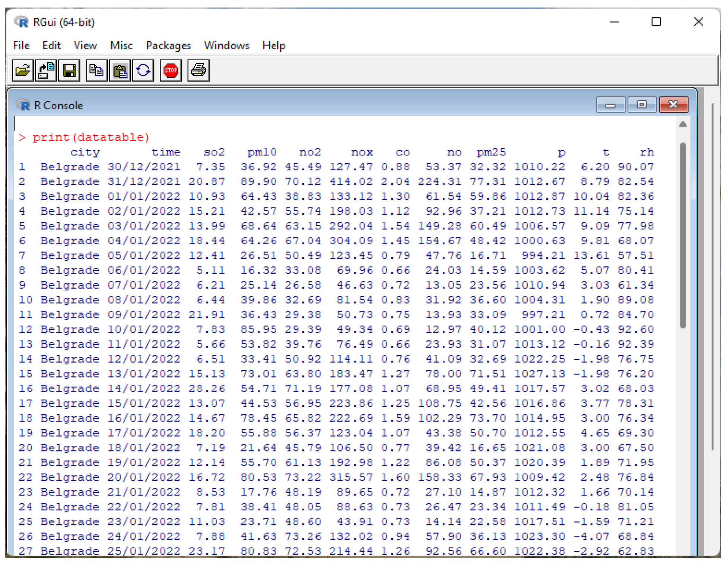
The obtained sample data from the web site as a source was transformed into a tab-delimited text file, suitable for loading into the R GUI (Figure 2), with a data structure consisting of city/time/SO₂/NO₂/NO_X/CO/NO/PM2.5/PM10/p/T/rh. The T symbol is regularly used for temperature, while in this research, the sample presents temperature with the symbol t. Data vectors, created from the loaded text file, are used to obtain a linear regression function that establishes the correlation of measured values of two air pollutants.

Figure 2. Air pollutants and meteorological measured values loaded into the R GUI.

The created R program enables the creation of linear regression functions (on all pairs of air pollutants and meteorological parameter values), graphical representation of data correlation in the form of colorized correlation heat maps and linear regression diagrams, as well as the use of linear regression functions and R language functions for the prediction of air pollution data. Finally, results of data processing (i.e., air pollutant value prediction) are organized according to categories of air pollutant concentrations and air quality: excellent, good, acceptable, polluted, very polluted, as defined by the Environmental Protection Agency [48].

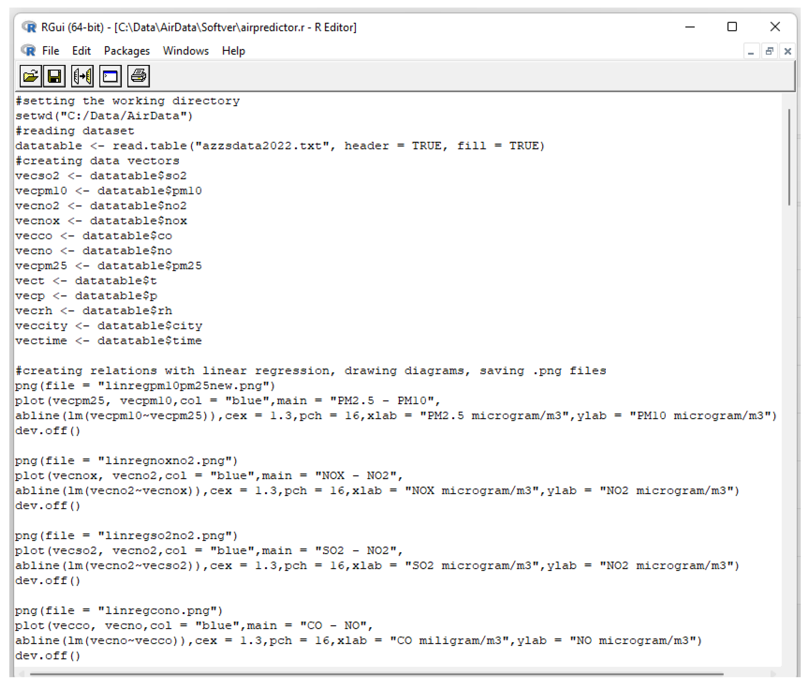
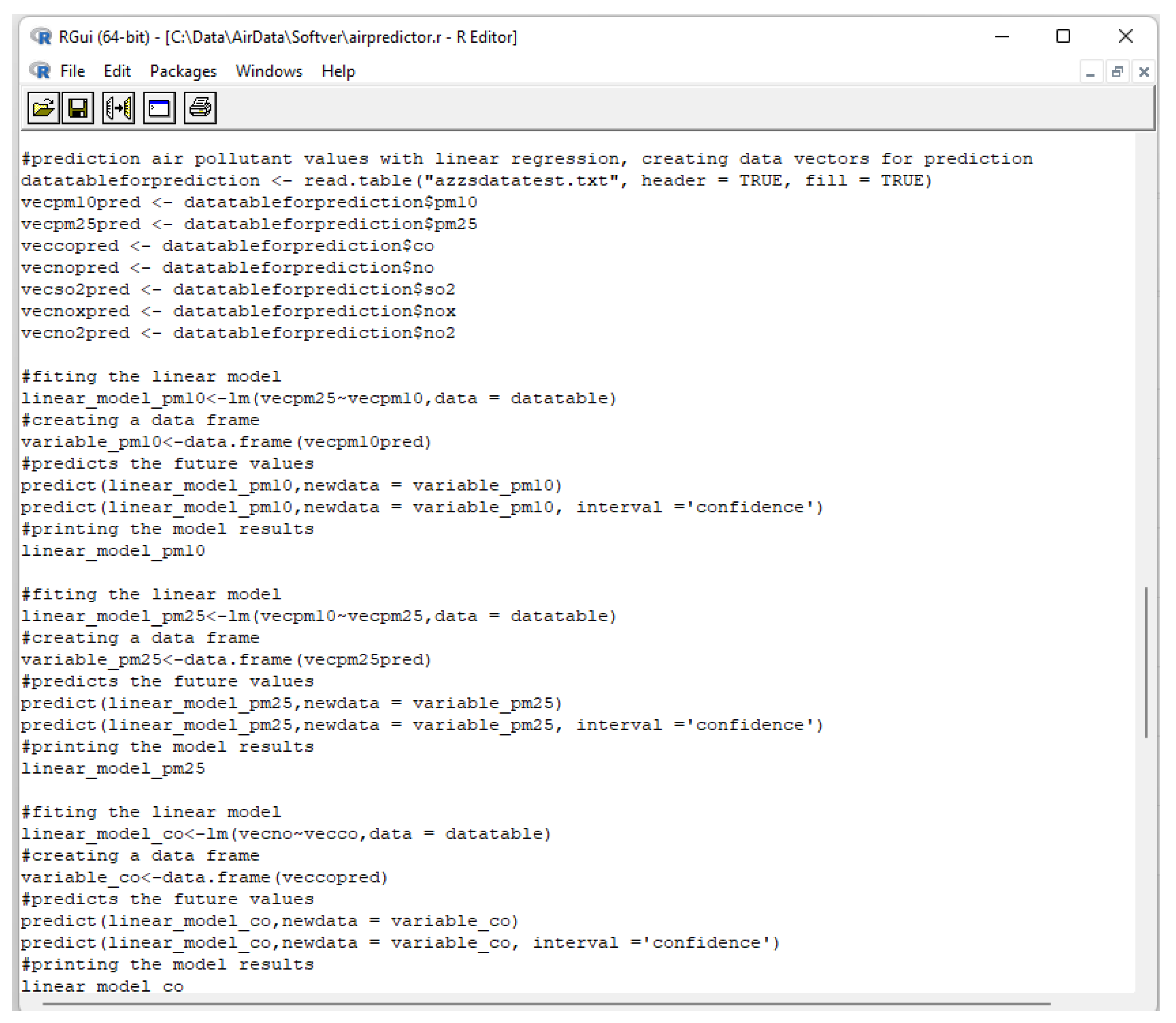
The program used in this research was written using the R programming language within the R GUI (graphical user interface) editor, created by R Team (The R Foundation for Statistical Computing c/o Institute for Statistics and Mathematics, Vienna, Austria) [16]. Figure 3 and Figure 4 present the first and second parts of the created R program within the R GUI development environment, respectively.

Figure 3. Created the first part of the R program with creating data vectors, relations with linear regression, and drawing diagrams in the R GUI.

Figure 4. Created the second part of the R program, which deals with predicting air pollutants values, fitting the linear model, and printing the results.

The first command in the newly created R program is used for setting the working directory in R with the setwd(path) procedure. The second command is reading data from an external tab-delimited .txt file that includes the stored data about air pollutants and meteorological conditions measured values with the read.table() function. It creates a table data structure with a title row that contains names for each column. The third step is creating vectors for measured pollutant values from the previously created table with the “<-“ operator for assigning values to R structures:

vector <- datatable$columnname

In this program, we created vectors for all pollutants and measured temperature, pressure, and relative humidity.

Establishing relations with linear regression between pollutants was conducted with the “lm()” function in R (Figure 3):

lm (vectorpollutant2~vectorpollutant1), where vectorpollutant1 is x and vectorpollutant2 is y in the linear function y = ax + b.

Drawing diagrams for the obtained mathematical models was completed with three commands (Figure 3). First, we defined a .png image with a name:

png (file = “imagefilename.png”)

After this command, the plot function creates the diagram based on the results of the lm function, while the dev.off function saves the diagram in a file named with the png command and stored at the location defined by the setwd command.

Predicting air pollutant values is possible with a predictor vector, response vector, and linear regression function (Figure 4). Commands for this purpose are listed below:

linear_model <- lm (vectorpollutantA~vectorpollutantB,data = datatable)

variable_vectorpollutantB<- data.frame(vectorpollutantBprediction)

predict (linear_model,newdata = variable_vectorpollutantB)predict (linear_model,newdata = variable_vectorpollutantB, interval = ‘confidence’)

A linear model is created by applying the lm function to two datasets (data vectors), where the first parameter will have the y role and the second parameter data vector has the x role in the resulting linear function. The linear model is a mathematical function representing the data vectors correlation. The predict() function from the R language was used to predict the future values based on the previously created linear model and prediction input data vector. For the purpose of prediction, another data vector was prepared as an input data set of air pollutant values or meteorological data. Upon these data, as well as with the linear model, the predict() function of the R language was used to derive the predicted values. The next step was to execute the predict() function again, this time with the third parameter of the function call being used for checking the “confidence” level in predicted values, i.e., to enable the calculations of prediction accuracy, i.e., the preciseness of the mathematical model obtained with linear regression (Figure 4). Finally, the summary command in R provides statistics related to the obtained linear model as well as statistics related to prediction fitting (i.e., a statistical computation of the accuracy of the computed mathematical model that was used for prediction).

4. Results and Discussion

Comparing to previously published works, where R was used for other ecology-related research, air pollution data was processed with special R packages, and linear regression was used for other purposes, and the diversity of software tools and technologies, this work contributes with the detailed presentation of a specially created R program by using R Language statements, and this program enables data correlation with linear regression, fitting of the derived mathematical functions, and prediction of air pollution data.

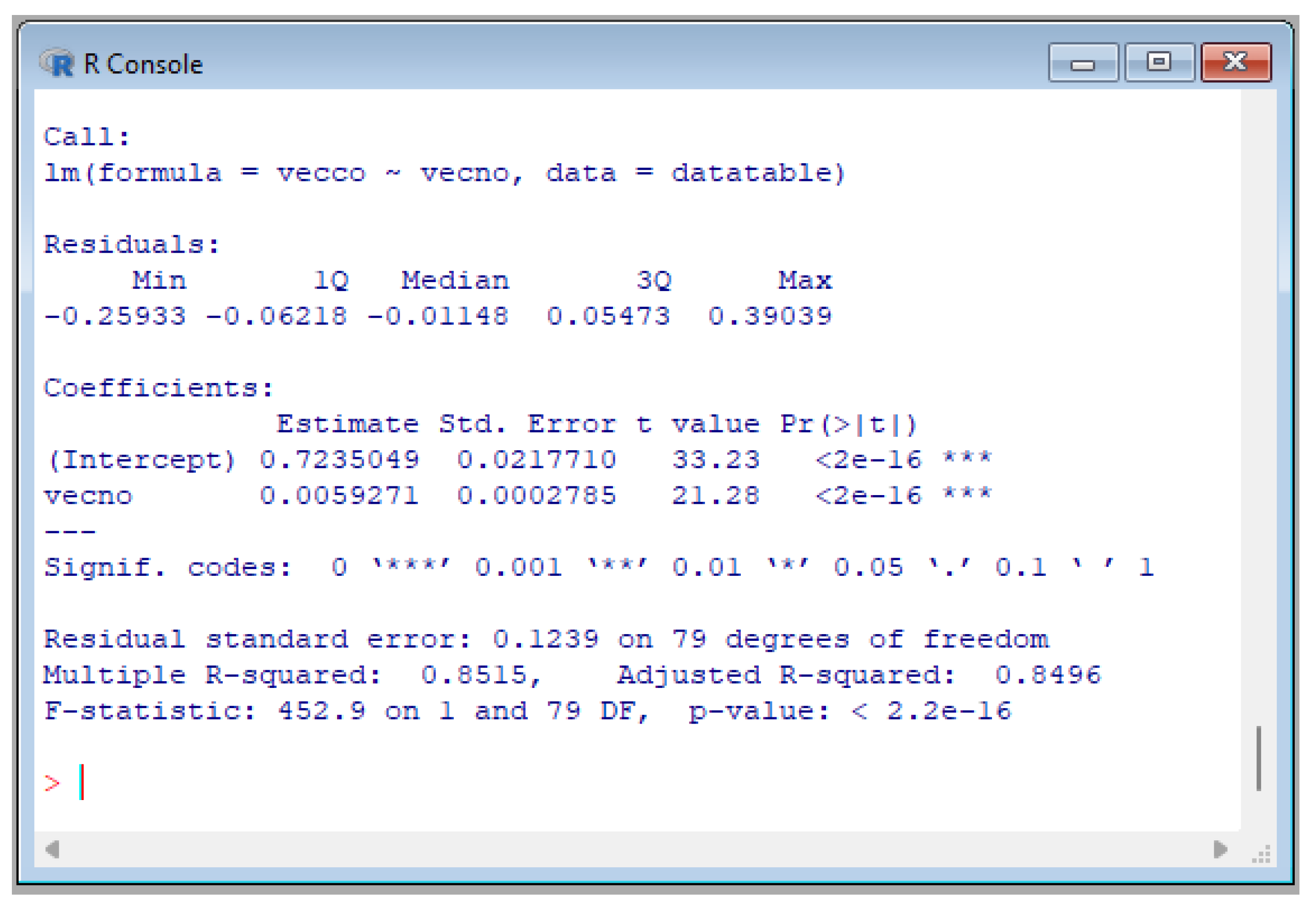
Results of executing the R program in processing linear regression and prediction statistics are presented with one example for CO (dependent) and NO (independent) data vectors at Figure 5 and Figure 6.

Figure 5. Example of R program execution for linear regression upon CO and NO pairs or vectors and the resulting statistics regarding mathematical model accuracy.

Figure 6. Example of results from executing the predict function for CO data vectors based on correlation with NO (within the execution of the created R program).

From Figure 5, it could be concluded that the r (correlation coefficient) for CO values being predicted from NO values has a value of 0.8515, which could be categorized as a high level of correlation.

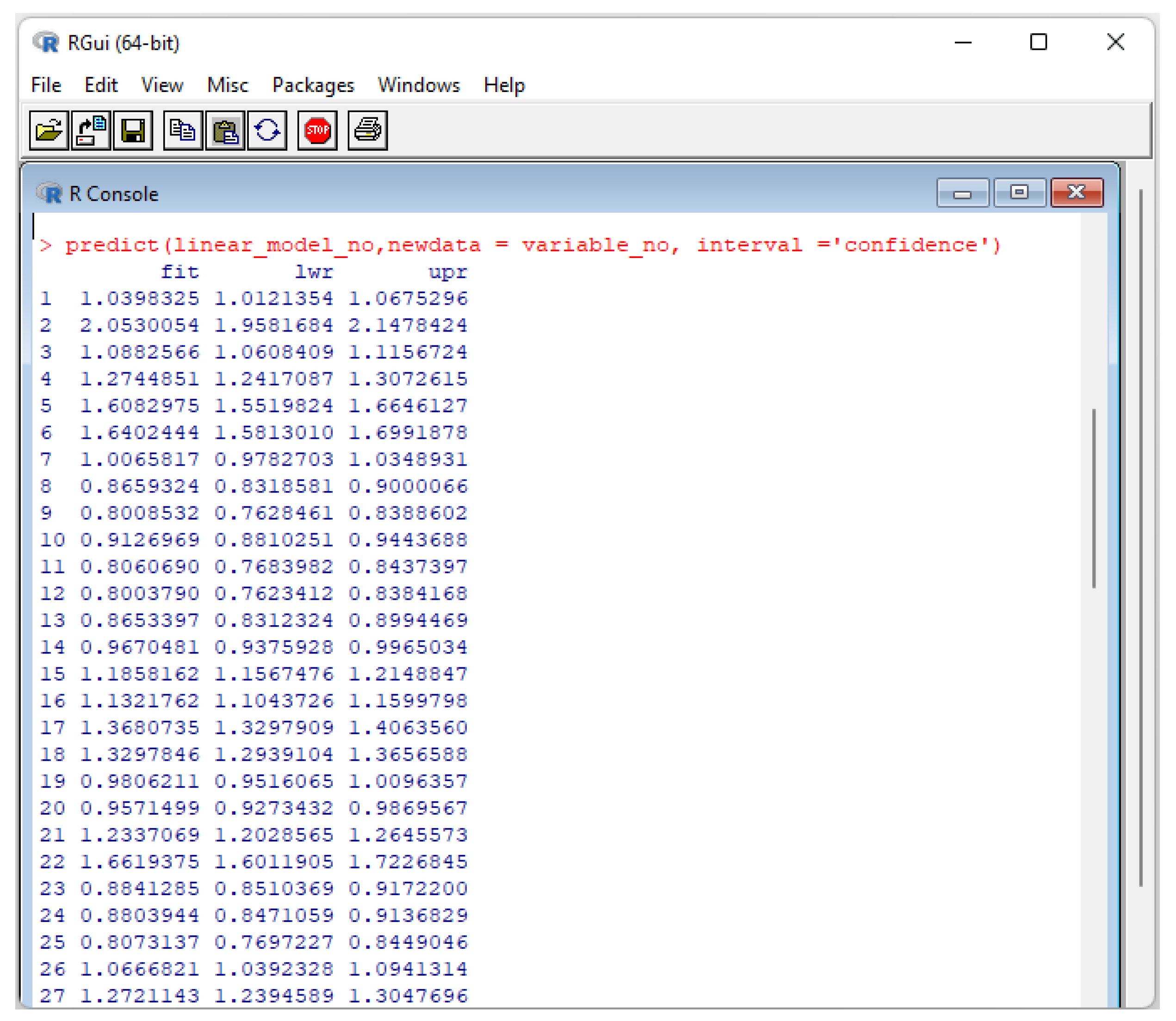
Results of executing the created R program (that includes utilization of the predict() R function) within the R GUI are shown in Figure 6. This is an example of successfully predicting future values of a CO pollutant based on the previously generated linear model of correlated CO and NO. Figure 6 presents three columns of data generated by the predict function for each item of the input data vector; there are computed values of prediction fit, but also lwr (lower) and upr (upper) values for each fit value. This way, it is obvious that the prediction function does not provide only one value, but an interval of values that could be expected in the future, using the underlying linear function as a basis.

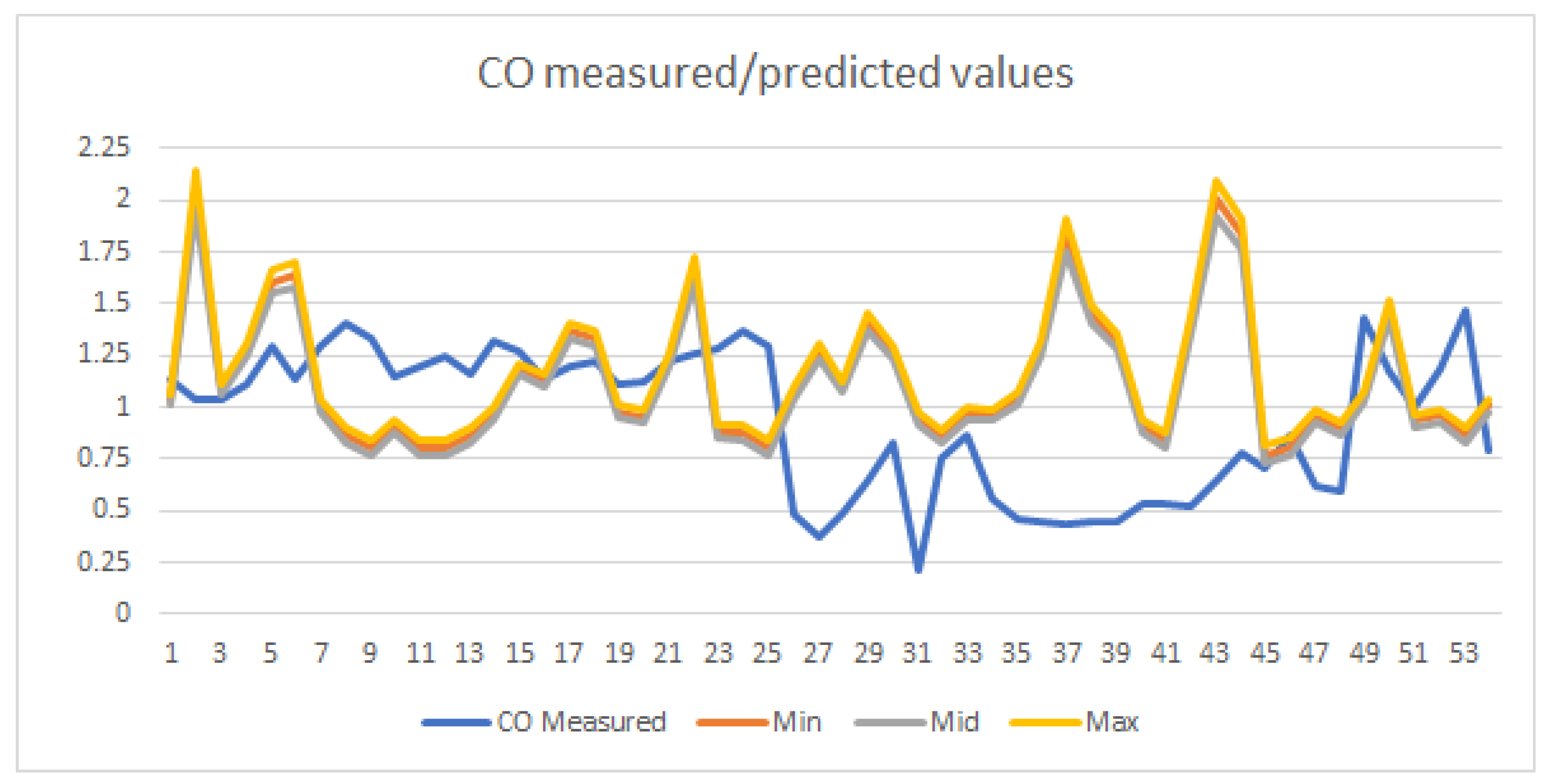
For this particular case of correlation between CO and NO values, Figure 7 presents a diagram that enables comparison between the computed prediction data and the real measurement data for CO as being dependent on the NO values data set in the previously presented prediction function.

Figure 7. Diagram of comparatively presented real measurement data of CO and predicted values (range) of CO, based on linear correlation with NO values.

Figure 7 contains graphs representing predicted data for CO for each particular measurement of NO as a lower (min), fit (mid), and upper (max) predicted value, as well as a graph presenting CO measured values (at the same time and at the same monitoring station as the NO value that was used for prediction). Since the r correlation coefficient between NO and CO is 0.8515, it is obvious from Figure 7 that the measurements and prediction graphs for CO are not very closely aligned.

The correlation heat map, presented at Figure 8, shows values of r correlation coefficients computed upon pairs of data vectors for all obtained parameters, including air pollutants and meteorological parameters.

Figure 8. Correlation heat map with all obtained air pollution parameters from the sample.

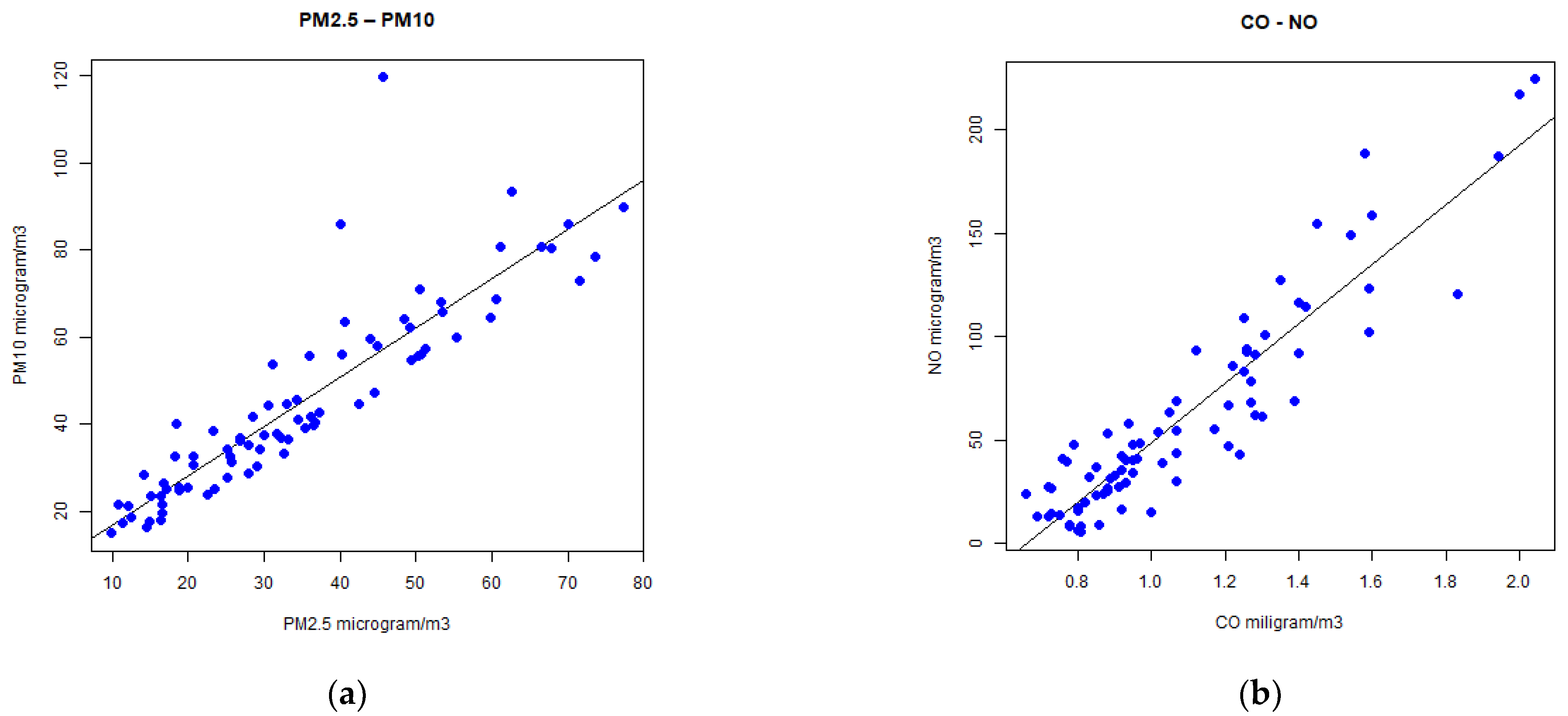
According to the correlation heat map, the high correlation (r values from 0.9 to 0.7) was computed with pairs NO-NO_x (r = 0.9809), CO-NO_x (r = 0.8667), NO-CO (r = 0.8515), PM2.5-PM10 (r = 0.7895), NO₂-NO_x (r = 0.7558), while for moderate correlation (r values from 0.7 to 0.5), there are also six air pollutant pairs. It could be concluded that the computed correlation between meteorological parameters and air pollutants is very low, with an r value less than 0.2. Therefore, in the rest of this paper, these pairs of parameters will not be presented with linear regression diagrams, predictions, and detailed statistics. The linear equations (as results of the linear regression method) are presented for selected (from the high, moderate, and low correlation categories) pairs of air pollutants as bivariate graphical plots (Figure 9a–f) that describe their mutual dependence, i.e., inter-variable correlations. Dots represent data from vectors, while lines, plotted between dots are the graphical representation of a derived linear equation from the data in vectors. A detailed statistical analysis of the correlation between the model and the data, apart from the graphical representation (quantity of dots placed near the line), can also be conducted on the basis of the statistical data presented in Table 1, Table 2, Table 3, Table 4, Table 5 and Table 6.

Figure 9. Linear regression diagrams created within R GUI with R program (a) PM10-PM2.5; (b) CO-NO; (c) SO₂-NO₂; (d) NO-NO_X; (e) CO-NO₂; (f) NO₂-NO_X.

Table 1. Summary statistics from linear regression model for PM2.5 and PM10.

Y = 3.413 + 0.698x					r = 0.7895
PM2.5-PM10 (x-Y)	Std. error	t-value	p-value	Residual Std. error	F-statistic
	0.0405	17.214	<2 × 10−16 ***	7.945	296.3

Signif. codes: 0 ***.

Table 2. Summary statistics from linear regression model for CO and NO.

Y = 143.66x − 94.94					r = 0.8515
CO-NO (x-Y)	Std. error	t-value	p-value	Residual Std. error	F-statistic
	6.751	21.28	<2 × 10−16 ***	19.3	452.9

Signif. codes: 0 ***.

Table 3. Summary statistics from linear regression model for SO₂ and NO₂.

Y = 0.229x − 0.328					r = 0.4468
SO2-NO2 (x-Y)	Std. error	t-value	p-value	Residual Std. error	F-statistic
	0.02873	7.988	9.18 × 10−12 ***	4.084	63.82

Signif. codes: 0 ***.

Table 4. Summary statistics from linear regression model for CO and NO₂.

Y = 8.428 + x39.489					r = 0.6305
CO-NO2 (x-Y)	Std. error	t-value	p-value	Residual Std. error	F-statistic
	3.401	11.609	<2 × 10−16 ***	9.722	134.8

Signif. codes: 0 ***.

Table 5. Summary statistics from linear regression model for NO and NO_X.

Y = 36.108 + 1.755x					r = 0.9809
NO-NOX (x-Y)	Std. error	t-value	p-value	Residual Std. error	F-statistic
	0.02757	63.64	<2 × 10−16 ***	12.27	4050

Signif. codes: 0 ***.

Table 6. Summary statistics from linear regression model for NO₂ and NO_X.

Y = 4.822x − 104.375					r = 0.7558
NOX-NO2 (x-Y)	Std. error	t-value	p-value	Residual Std. error	F-statistic
	0.3084	15.637	<2 × 10−16 ***	43.83	244.5

Signif. codes: 0 ***.

Standard statistical parameters such as Fisher’s criterion (F), correlation coefficient (r), estimate and residual standard error, p-value, and t-value were used for model validation. According to statistical parameters, it can be seen from Table 1, Table 2, Table 3, Table 4, Table 5 and Table 6 that we have a moderate, high, and very high positive correlation with the model. The best correlation and fit to the data is with NO-NO_X pollutants (r = 0.9809), which had a high F-value and low p-values and standard errors. The correlation between CO and NO pollutants was strong (r = 0.8515), which can be seen by statistical parameters and a graph. The very high correlation was in the case of PM2.5-PM10 (r = 0.7895) and NO₂-NO_X (r = 0.7558), as were the high F-value and low p-value and standard errors. CO-NO₂ air pollution showed a moderate correlation with the model (r = 0.6305). The weakest interdependence was shown by SO₂-NO₂ pollutants (r = 0.4468), who had the lowest F-value and the greatest dispersion of data.

A good correlation between NO₂, NO, and NO_X (r~0.68 to 0.98) can be explained by the chemical similarity of the compounds and the chemical pathway of their formation [49].

N₂ + O₂ → 2NO,

(1)

NO + O → NO₂,

(2)

NO + O₃ → NO₂ + O₂,

(3)

According to the correlation heat map (Figure 8), there is a weak correlation (r < 0.5) between chemically different oxides of carbon, sulphur, and nitrogen. The specific case is CO, which establishes a high and medium correlation with all air pollutants, except with SO₂ (r = 0.3349).

Table 7 shows the summarized and categorized results of predicting air pollutant values for SO₂, PM10, PM2.5, CO, and NO₂. Part of the data that is the source for Table 7 was previously presented in Figure 8. The categorization of program execution results (prediction data), which is presented in Table 7, has been performed according to air pollutant concentration indexes as excellent, good, acceptable, polluted, much polluted, and colored according to criteria defined by the Environmental Protection Agency of the Ministry of Environmental Protection, Republic of Serbia [48], which are aligned with the normative defined in the European Union. These values are, of course, different for each pollutant.

Table 7. Summarized and categorized results of predicting air pollutant values with R.

Air Quality Index	Excellent	Good	Acceptable	Polluted	Very Polluted
PM2.5 concentration intervals number of predicted values (relation with PM10) (µg/m3)	0–15	15.01–30	30.01–55	55.01–110	>110
	3	36	33	9	0
NO2 concentration intervals number of predicted values (relation with SO2) (µg/m3)	0–50	50.01–100	100.01–150	150.01–400	>400
	46	35	0	0	0
CO concentration intervals number of predicted values (relation with NO) (mg/m3)	0–5	5.01–10	10.01–25	25.01–5	>50
	81	0	0	0	0
SO2 concentration intervals number of predicted values (relation with NO2) (µg/m3)	0–50	50.01–90	90.01–180	350.01–500	>500
	81	0	0	0	0
PM10 concentration intervals Number of predicted values (relation with PM2.5) (µg/m3)	0–25	25.01–50	50.01–90	90.01–180	>180
	16	37	27	1	0

Note: Categories colors according to [48].

According to the results presented in Table 7, it could be concluded that the great majority of predicted values could be categorized as excellent or acceptable.

5. Conclusions

This paper contributes to the R program that enables data transformation, linear regression, mathematical model fitting, and the processing of prediction functions. This program also enables the graphical presentation of results in the form of diagrams that illustrate the correlation between pollutants. This research also contributes to the evaluation of linear regression functions for their accuracy. It has been shown that the resulting functions enable predictions with high precision; the predicted values correlate very well with the obtained data. The developed R program was created with R language statements without using specific R packages. Therefore, it could be used or easily adapted to diverse application domains. The second contribution is related to the results of data correlation with all types of air pollutants, which are included in most frequent air quality monitoring systems. It has been shown that certain air pollutant pairs of data have a high level of correlation since their linear regression function has a high level of fitting. The limitations of this work are related to several aspects. The R program was not presented entirely in this paper (because of the program’s length), but it is available at the public repository GitHub, and only the most important lines of R code are presented and explained. The second limitation is related to the sample characteristics: one city, two years, and only a winter period of three months in both years; not all atmospheric parameters were included (e.g., data from monitoring stations in this sample do not provide wind-related data). Future work could be related to the utilization of the created R program to make predictions based on a wider set of parameters, larger data sets taken over longer periods of time, a diversity of monitoring locations, adaptation to other application domains, and improving the program to use other statistical methods supported by the R language, with a special emphasis on supporting further chemical analysis of complex interactions and processes with gasses in the atmosphere.