Abstract
Assigning predefined classes to natural language texts, based on their content, is a necessary component in many tasks in organizations. This task is carried out by classifying documents within a set of predefined categories using models and computational methods. Text representation for classification purposes has traditionally been performed using a vector space model due to its good performance and simplicity. Moreover, the classification of texts via multilabeling has typically been approached by using simple label classification methods, which require the transformation of the problem studied to apply binary techniques, or by adapting binary algorithms. Over the previous decade, text classification has been extended using deep learning models. Compared to traditional machine learning methods, deep learning avoids rule design and feature selection by humans, and automatically provides semantically meaningful representations for text analysis. However, deep learning-based text classification is data-intensive and computationally complex. Interest in deep learning models does not rule out techniques and models based on shallow learning. This situation is true when the set of training cases is smaller, and when the set of features is small. White box approaches have advantages over black box approaches, where the feasibility of working with relatively small sets of data and the interpretability of the results stand out. This research evaluates a weighting function of the words in texts to modify the representation of the texts during multilabel classification, using a combination of two approaches: problem transformation and model adaptation. This weighting function was tested in 10 referential textual data sets, and compared with alternative techniques based on three performance measures: Hamming Loss, Accuracy, and macro-. The best improvement occurs on the macro- when the data sets have fewer labels, fewer documents, and smaller vocabulary sizes. In addition, the performance improves in data sets with higher cardinality, density, and diversity of labels. This proves the usefulness of the function on smaller data sets. The results show improvements of more than 10% in terms of macro- in classifiers based on our method in almost all of the cases analyzed.
1. Introduction
In the age of information explosion, processing and classifying enormous amounts of text data manually is time-consuming, and it is a huge challenge to automate this task using computational methods. Furthermore, the performance of manual text classification can be easily influenced by human factors such as experience and fatigue. This requires the use of machine learning methods to speed up text classification processing and to obtain less subjective and more reliable results. In addition, this can also aid in improving efficiency in information retrieval and to alleviate the problem of information overload in locating the required information.
The problems related to the classification of multilabel text exists in different domains. Even though the basic models normally assume the existence of two classes, they have been extended to problems with more than two classes and multilabel, which are closer to real applications.
Although there has been an exponential increase in the number of publications based on deep learning models in recent years, it is not possible to completely rule out the techniques and models based on shallow learning. Today there is a debate between the “white box” vs. “black box” approaches, with advantages and disadvantages for both. Superficial learning highlights the feasibility of working with relatively small data sets and interpretability. Deep learning models stand out for their robustness and good performance.
The aim of this research is to evaluate a new term weighting function called relevance frequency for a label (), initially introduced in [1] for tf-rfl, and extended and deepened in [2] as bin-rfl. This document presents greater maturity than previous papers, which were previously presented at conferences and in journals, and has a better foundation as well as, a better description of the proposed modification and an improved analysis of the results. Likewise, the analysis of relevant characteristics in the data sets is deepened for a better understanding of the method and choice of the representation. The impact of rendering is shown by considering different performance measures for multilabel classification problems. For this, two types of linear classifiers used in these type of problems were used; these are: Linear Support Vector Machine (SVM) and one-layer artificial neural networks (ANN). The use of linear classifiers allows for the evaluation of the improvements in the performance of the algorithms just by modifying the input space by means of the new representation.
The contribution of this research lies in the proposal of a simple and interpretable representation that combines ensemble machine learning and shallow classification models. The aim of this new representation is improved classifier performance. Testing of the proposed representation was carried out on ten multilabel text data sets that are widely referenced in the literature, obtaining alternate performance measurements.
This document is structured as follows. In Section 1, the subject is introduced, in Section 2, the state of the art is presented. In Section 3, the proposal is presented, and in Section 4, the applied methodological framework is described. The experimental results are described in Section 5, where the results are discussed and the performance of the proposal is compared with other models. The Section 6 presents the final conclusions and future work.
2. Related Work
2.1. Text Classification Problem
Text classification (TC), also known as text categorization, is the activity of assigning labels to natural language texts based on a set of predefined categories. TC was created in the early 1960s, but only in the early 1990s did it become an important subfield of the information systems discipline, thanks to the wide field of applications and the growth in computing power.
The main goal of classification is to take a vector x as input and to assign it to one of the K discrete classes where k = 1, …, K. In the most common scenario, the classes are taken to be disjointed [3] such that each entry is assigned only one class. Therefore, the input space is split into decision regions whose boundaries are called decision boundaries or decision surfaces.
Text data are different from numeric, image [4,5], or signal data [6] and others data type [7,8,9,10]. Therefore, texts must be preprocessed using Natural Language Processing (NLP) methods in order to be delivered to the model. Shallow learning models generally need to obtain good features from the examples using different methods and then to classify them with classical machine learning algorithms. Therefore, the effectiveness of the classification method is largely dependent on the extraction of text features. Unlike shallow models, however, deep learning integrates feature extraction into the model fitting process by learning a set of nonlinear transformations that are used to assign features directly to the results.
From the 1960s to the 2010s, shallow learning-based text classification models dominated. In [11] it is stated that the first methods based on statistical models (shallow learning), such as Naive Bayes [12], K-Nearest Neighbor [13], and Support Vector Machine [14] dominated up to the year 2010. Compared with previous rule-based methods, this method has obvious advantages in terms of Accuracy and stability. This approach needs to perform feature selection, which can be time consuming and costly. Since the 2010s, text classification has been evolved through the use of deep learning models. Compared to methods based on shallow learning, deep learning methods avoid the design of rules and features by humans, and automatically provide semantically meaningful representations for text analysis. However, deep learning-based text classification is data intensive and computationally complex.
TC is now being applied in many contexts, ranging from document indexing based on a controlled vocabulary, to automated metadata generation, word sense disambiguation, document filtering, the hierarchical catalog population of web resources, and, in general, any application that requires document organization or adaptive document selection and dispatch.
Shallow learning-based methods learn from data, where the representation of text features is very important for achieving good classification performance. However, it requires the development of feature selection. Before training the process used for the classifier, we need to gather knowledge or experience to extract features from the original text. Shallow learning methods train the initial classifier based on various textual features extracted from the raw text. For small data sets, shallow learning models generally outperform deep learning models under the limitation of computational complexity. Therefore, some researchers have studied the design of shallow models for specific domains with less data. Furthermore, deep learning models can learn feature representations directly from the input without almost any manual intervention and prior knowledge. However, the deep learning methodology is a data-driven method, which generally needs a large amount of data to achieve high performance. Typically, much more data are required than traditional machine learning algorithms, which means that this technique cannot be applied to classification tasks on small [15] data sets. In addition, the huge amount of data required for deep learning classification algorithms further exacerbates the computational complexity during the [16] training step. Finally, the lack of interpretability of these models does not make them comparable with superficial models to explain why and how it works well.
Both shallow and deep models can achieve good performance in most text classification tasks. However, the interpretation of the deep models is still a challenge.
In recent years, researchers have developed many approaches to improve the accuracy of text classification models. However, when there are some complex examples in the data sets, the performance of the model decreases significantly. Consequently, the relationship between effectiveness and efficiency in models, and how to improve the robustness of models, is a challenge and a focus of current research.
Deep learning models have unique advantages in feature extraction and semantic mining, and have achieved excellent results in text classification tasks. However, deep learning is a black box model, the training process is difficult to reproduce. Likewise, the understanding of the implicit semantics and the interpretation of the results are pending challenges.
Shallow learning models improve text classification performance primarily by improving the feature extraction scheme and classifier design. In contrast, the deep learning model improves performance by learning the implicit features of the raw data and the structure of the model, as well as additional data and the knowledge that it uses in previous phases.
Moreover, the interpretability of deep learning models, especially Deep Neural Network, has always been a limiting factor for use cases that require explanations of the features involved in the modeling, and such is the case for many prescriptive models applied to healthcare [17] or in automations that may affect the freedom of people [18,19]. The weights in neural network models are a estimation of how strong each connection is between each neuron in finding the important feature space. As a result, complex algorithms such as deep learning are difficult to understand.
2.2. Multilabel Text Classification
Traditionally, the classification (or categorization) of texts has been defined as assigning a Boolean value (true or false) to each pair , where D is the domain of the documents (corpus) and is the set of default labels (classes). If a document is categorized under only one label, that is, in some partition of the set of classes (non-overlapping categories) or under multiple labels at once (overlapping categories), it is called a ‘one-label problem’ or a ‘multilabel problem’, respectively [20]. The most commonly studied case to solve text classification problems is that of ‘one-label’, and the main approach is the so-called Binary Classification (BC), where a document is classified either to the category or its complement (). This approach can be extended and used to solve problems with more categories.
Interest in the classification of multilabel texts has increased in recent years. Among the proposals presented by [21], the most commonly used approach is the so-called transformation of the problem. In a multilabel problem, there exists a finite number of labels , where corresponds to the j-th label, and to the set of documents labeled , where represents the feature vector and is the set of labels for the i-th text.
Table 1 presents an example of multilabel texts. It represents that Text 1 belongs to the classes ‘Sports’ and ‘Politics’, that Text 2 belongs to the classes ‘Sciences’ ‘Politics’, that Text 3 belongs only to the class ‘Sports’, and finally that Text 4 belongs to the classes ‘Religion’ and ‘Sciences’.

Table 1.
Representation of a Set of multilabeled Examples.
The approaches to solving this problem can be classified into two approaches: the transformation of the problem and the adaptation of the model [21]. The transformation approach to the problem is algorithm-independent, that is, it transforms the multilabel learning task into a single-label classification task. Consequently, this technique may be used via current methods. The most common problem transformation method, called Binary Relevance (BR), learns binary classifiers , one for each different label in L. Through the use of Binary Relevance, the original data set is transformed into data sets . Each labels each instance of text in D with if is contained in the instance, or if the text example does not contain the tag. BR provides the same solution for both single-label problems and multilabel problems using binary classifiers. For the classification of a new instance x, this method generates a set of labels as the union of the labels generated by the classifier . This is usually the most common transformation, and it is the same solution used when trying to deal with a multi-class classification problem using binary classifiers (see Table 2).
Table 2.
Resulting Transformation using Binary Relevance.
Another type of transformation of the problem is called a Label Powerset (LP). In this transformation, each set of labels is considered as a new category. Then, if we have LP combinations, it is possible to use binary classifiers, one for each new label. The data set is handled as a single-label type, and then a single-label classifier with multiple disjoint classes is built (see Table 3).
Table 3.
Resulting Transformation using Label Powerset.
The second method deals with adapting some specific learning models and algorithms so that they can handle the multilabeled data directly. These adaptations are achieved thanks to model adjustments, such as modifications to the classical formulations of statistics or information theory. The preprocessing of the documents to achieve a better representation can also be considered within this type of transformation.
The classification of multilabel texts has also been approached by means of algorithms, which directly capture the characteristics of the multilabel problem. The authors of [22] propose a method based on fuzzy logic, where a multilabeled text can belong to one, or more than one category. The authors state that by incorporating fuzzy techniques, the method can overcome problems caused by high memory requirements or low performance. The authors of [23] focus on solving the limitations of the Backpropagation Learning algorithm so that it can work with multilabeled data, and propose Backpropagation Multilabel Learning (BP-MLL). In this proposal, a very simple neural network approach is used for large-scale multilabeled text classification tasks.
The authors of [24] propose a model based on graph attention networks to capture the dependency structure between labels (MAGNET). The results of the proposed model are validated on five real-world MLTC data sets. The proposed model achieves a similar or better performance compared to the previous models of the latest generation. The MAGNET model framework uses attention layer graphs for classification to generate the inputs for a BiLSTM to generate the feature vectors that are encoded by the embeddings of the BERT [25] model. The input to the attention network graph is an adjacency matrix and the label vectors. The GAT output are label features that are applied to the feature vectors obtained with BiLSTM. It uses performance metrics that does not allow a person to evaluate its performance on unbalanced data sets. MAGNET’s proposal improved performance marginally over traditional models, such as Binary Relevance and Chain Classifiers.
In [26], the Label-Wise Pre-Training (LW-PT) method is suggested for obtaining a document representation that includes label information. It is expected that the linked labels always co-occur in related documents, and for this, a multilabel document is represented as a composite of various label representations. By creating document-label classifiers and instructing document-label coders, LW-PT puts this concept into practice. The previously trained label encoder fine-tunes. The experimental results support the suggested approach in two sets of data, and only a few evaluation measures are used to compare it to conventional approaches.
On the other hand, ref. [27] proposes a global hierarchical model for the classification of multilabeled texts, which seeks to take advantage of the dependency relationships between labels. In line with the exploitation of Deep Learning, ref. [28] proposes a model for extreme multiple label text classification, facing the problem of assigning to each document the most relevant subset of class labels of an extremely large collection of labels, where the number of labels could reach hundreds of thousands or millions. The work in [29] also uses an estimation of the distribution of categories in a non-linear embedding space in a model called Prototypical Networks for multilabel Learning (PNML), and [24] proposes Classification Neural Networks (CNN), different from Convolutional Neural Networks, as a new approach based on deep learning to face the label hierarchy problem.
Regardless of the solution approach to the multilabel problem and the algorithms that solve it, according to [14], any text classification task has complexities because the feature space is highly multidimensional, a heterogeneous use of the terms, and a high level of redundancy. Multilabel problems have additional complexities, including a large number of labels and the imbalance of labels across the document set.
Although traditional measures of evaluating the performance of classifiers, such as the macro- and Hamming Loss measures are useful in multilabel cases, new evaluation measures have also emerged with the intention of analyzing the performance of classifiers, and the performance in assigning the set of labels that correspond to each document, such as the accuracy of the set of labels, a measure called Label-Set Accuracy [30].
2.3. Text Representation
The performance of a case-based reasoning system depends largely on the representation of the problem. The same task can be easy or difficult, depending on the way it is described [31]. The explicit representation of relevant information tends to increase the performance of machine learning. In this way, through a more complex representation, better results could be obtained with simpler algorithms. In line with this, mechanisms that allow for the selection and weighing of the characteristics that improve the performance of a classifier in specific contexts are being proposed [32]. Likewise, this is the case with those who propose the analysis of the visual elements of the text as an additional feature [33].
In the particular case of documents, the representation of the text has a high impact on the [34] classification task. The vector space model is one of the most commonly used models for information retrieval, mainly because of its conceptual simplicity and the attractiveness of its underlying metaphor of using spatial proximity for semantic proximity [35]. In the vector space model (VSM), the contents of a document are represented by a vector of terms , where k is the size of the set of terms (or features). Some elements used in the representation of a text are the N-grams, words, phrases, the logic of terms and declarations, or any other lexical, semantic, and/or syntactic unit that can be used to represent the content of the text.
Regardless of the characteristics used to represent a text, from the existence of these characteristics, it will be determined as to which classes the text belongs. If only the existence of the characteristic is considered or if the frequency of occurrence of that characteristic is considered, then two models can be distinguished, which [36] calls the Bernoulli Multivariate Model and the Multinomial Model, respectively.
The Multinomial Model indicates that a document is represented by the set of occurrences of terms in the document. The order of the terms is lost; however, the number of occurrences of each term in the document is captured. If a Bayesian model is used, when calculating the probability of a document, the probability that the terms appear is multiplied. Here, the occurrences of individual terms can be understood as the events, and the document as the collection of term events. The most widely used measure is the relevance indicator , which is used to represent how much the feature or term t contributes to the semantics of the document d, and it can have values of between zero and one ([0, 1]).
For its part, the Bernoulli Multivariate Model specifies that a document is represented by a vector of binary attributes that indicates which terms occur and which terms do not occur in the document. The number of times a term appears in a document is not captured. As in the previous case, if a Bayesian model is used, when calculating the probability of a document, the probability of all attribute values is multiplied, including the probability of the non-occurrence of terms that do not appear in the document. Here, it can be understood that the document is the event and the absence or presence of terms as attributes of the event. This describes a distribution based on a Multivariate Bernoulli Event Model. In this case, the flag is used, which takes the value of 1 when the term t exists at least once in the document d; that is, it can have a value of zero or one ({0, 1}). The factor based on the Bernoulli Multivariate Model is called a Binary Representation or a Boolean Model. Many problems, either by their nature or by the measurements that can be obtained from them, use the representation model based on the Bernoulli Multivariate Model [36].
There are different ways to describe the features of a text so that different text classifiers can work on them. Refs. [14,37], for example, combine transformations with different kernel functions on Support Vector Machines. On the other hand, according to [38], two important decisions must be made when choosing the representation based on the vector space model. (1) What should a term consist of? What should be a root word, a word, a set of words, or their meaning? (2) How should the term’s weighting scheme be? Weighting could be achieved via a binary or inverse document frequency (-) function developed by [39] using feature selection metrics such as chi-squared , information gain (), reason or profit ratio (), etc. Term weighting methods improve the effectiveness of text classification through an appropriate selection of term weights. Although text classification has been studied for several decades, term weighting methods for text classification are often taken from the field of information retrieval (), including, for example, the Boolean model, , and its variants. In general, to weight the terms in the vector space model, the frequency of the terms or the frequency of the documents containing a term can be used.
According to [40], many investigators have worked on the technique of extracting text features trying to maintain the syntactic and semantic relationship that is lost when only words are considered. Additionally, although many researchers have tried novel techniques to solve this problem, they still have limitations. A simple but expensive solution to the syntactic problem is to use the n-gram technique for feature extraction.
Term Frequency (TF)—which assigns each word a number according to the number of times that term appears in the whole corpus—is the most fundamental type of weighted word feature extraction. Word frequency is typically used as a logarithmically scaled or as the Boolean weight in techniques that scale TF findings. In all word weighting methods, each document is translated into a vector (with a length equal to that of the document) containing the frequency of the words in that document. Although this approach is intuitive, it is limited by the fact that certain commonly used words in the language can dominate such representations. In contrast, weighted word functions are based on word counts in documents and can be used as a simple word representation scoring scheme. Each technique presents unique limitations. Weighted words calculate document similarity directly from the word count space, increasing the computation time for large vocabularies. While single word counts provide independent evidence of similarity, they do not account for semantic similarities between words. Word embedding methods address this problem, but they are limited by the need for a huge corpus of text data sets for training. As a result, scientists prefer to use pre-trained word embedding vectors. However, this approach cannot work for words that are missing from these text data corpora.
2.4. Ensemble Methods
Ensemble training studies the use of integrating an ensemble of models to build a predictor that improves performance over a single, more complex model.
According to [41], there are two assumptions underlying model ensemble algorithms: the first is that a more accurate predictor can be built by combining models, rather than using a more complex model. Thus, the weighted average of the results of a collection of models could improve the prediction performance of a data set as a linear combination of them, and could generate a lower bias than any of the individual predictors (even being able to choose the best predictor individual).
The second premise suggests that the performance of an ensemble is better than a predictor based on a model. Usually, measures of loss, for example, quadratic loss, are not affected by a change in the model (if its predictions remain unchanged). Individual predictions are compared with each other, since they only depend on prediction and observation. In contrast, model-based approaches could violate the preeminence principle by confusing predictor construction with its performance.
Using multiple copies of an individual classifier produces no real improvement in the generalization of the ensemble and, therefore, it seems intuitive that when the predictors are combined, they need to have some degree of heterogeneity or diversity. The diversity of an ensemble can be implicitly promoted by modifying the data set for training the classifier, by modifying the architecture of the predictors, or by modifying the learning parameters. In contrast, explicit methods for constructing ensembles use a diversity metric that depends on the other members of the ensemble, though diversity is not necessarily guaranteed to contribute to improved ensemble performance.
Ensemble’s methods can differ over the course of three different stages: base classifier manipulation, data manipulation, and in the function that the committee uses to generate the consensus output.
3. Label-Dependent Representation
Although in recent years there has been a growth in the interest of the scientific community in deep learning models, there is a debate between the “white box” vs. “black box” approaches, with advantages and disadvantages of both approaches. Superficial learning highlights the feasibility of working with relatively small data sets and interpretability. Deep learning models stand out for their good performance and robustness. Therefore, it is not possible to completely rule out techniques and models based on shallow learning, especially when the set of training cases does not have a large volume of data and the set of features is not very extensive.
As already mentioned, in this approach, it is planned to use classification methods based on shallow learning combining representation modification with problem transformation. Although this research does not use classification methods based on deep learning, such as BERT and its variants, it would also be possible to use this approach to modify the characteristics of the representation of the original texts and generate to new layers or inputs to deep learning methods, especially when working with small data sets. This would also give better interpretability to the deep learning models.
On the other hand, in the case of the problem of multilabeled texts, the classification models must deal with data sets with a high cardinality, density, and diversity of labels. Cardinality measures the average number of labels associated with each document, density is the cardinality divided by the number of labels, and diversity represents the percentage of label sets present in the corpus divided by the number of possible label sets. In this work, we use data sets with a cardinality of between 1.18 and 3.28, a density of between 0.014 and 0.098, and a diversity of between 0.041 and 0.442.
In this section, the well-known tf-idf [39] representation is explained, and our proposed function for the weighting of rfl terms is presented. Based on the latter, we propose two new representations, one based on the Multivariate Bernoulli model called bin-rfl, and another based on the Multinomial tf-rfl model. In this type of representation, the indicator can have values of between zero and one ([0, 1]), is called the Multinomial Model by [36], and is different from the Bernoulli Multivariate Model, where the indicator is , which is represented by one when the term t exists at least once in the document d; that is, it can have a value of zero or one ({0, 1}). The factor based on the Bernoulli Multivariate Model is called a Binary Representation or Boolean Model. Many problems, either by their nature or by the measurements that can be obtained from them, use the representation model based on the Multivariate Bernoulli Model.
This raises the hypothesis that a supervised modification to the text representation that considers frequency representations or binary representations, together with a function for the supervised weighting of the terms that is based on the known examples, according to their labels, could improve the performances of the classifiers significantly. When referring to supervised modification, what we are proposing is a modification of the representation based on the analysis of the labeled examples of the training set, which is why it is supervised. For the term weighting method for multilabel problems, we will use as variables those described in Table 4: , which represents the number of documents in the category containing the term t and representing the number of documents in the category that do not contain the term t.
Table 4.
Variables used for weighting in a multilabel problem, given a term t and 4 categories.
3.1. Term Frequency-Inverse Document Frequency (-) Representation
According to [20], the most widely used text representation for text classification is - from [39]. This is where each component of the vector is calculated according to Equation (1):
where is the frequency of the term t in the document d. For the two-category problem, is the number of documents, and = is the number of documents that contain the term t.
The main contribution of this representation is that it weights with less importance the terms that are very frequent in the collection of documents through the factor .
3.2. Term Frequency-Relevance Frequency for a Label (-) Representation
In the research carried out by [1], the preliminary results of the representation Relevance frequency for a label, tf-rfl were presented. This representation is described in the following equation, as a new representation for multilabel problems.
where is the frequency of the term t in the document d, is the number of documents under the category under the evaluation l that contain the term t, and is the average number of documents containing the term t among the set of documents labeled in a category other than l, i.e. .
The constant value of 2 on the right-hand side of the formula is assigned because the base of the logarithmic operation is 2. Without the constant 2, it could have the effect of setting the other terms to zero. Other bases could be used for the logarithm function, which would also imply a modification of the value of this parameter.
The main contribution of this representation is that it weights with less importance the terms that are equally frequent in the different categories, and weights with greater importance the terms that are more frequent in the category under evaluation.
It is also possible to use - based on the Bernoulli Multivariate Model, instead of -, based on the Multivariate Model. In this case, instead of using , is used.
In order to evaluate the performance improvement due to the use of weighting, this paper will present a new representation based on the occurrence of terms in each document; that is, Binary Representation or Boolean Representation. This representation, based on the Multivariate Bernoulli Model, uses less information than the one based on the Multinomial Model, since only information on the existence or not of a word in the text is used, and not its frequency of appearance.
3.3. Multivariate Bernoulli Model—Label-Dependent (-) Representation
A new representation for the multilabel problem, which is proposed in this work, called -, is based on a representation of the Multivariate Bernoulli Model that is weighted using the frequency term of a label, and calculated as in Equation (3):
where takes the value of 1 if the term t is present in the document d, and 0, if the term t is not present in the document d; is the number of documents in the category under evaluation that contain the term t, and is the average number of documents that contain the term term t for each set of tagged documents other than l. This new representation helps to make a better distinction of the terms, which is reflected in a better performance classification, as will be seen in Section 5.
The term t weighting method here considers each term occurrence frequency within each group of documents with labels that are different from those of the document under evaluation. The occurrence measurement rfl, will be larger if term t is appears with higher frequency in documents with label than in documents with other labels. Moreover, the occurrence measurement will be lower if term t appears with higher frequency in documents with labels other than I. Therefore, the weighting rfl results a better discriminator among categories.
The modification of the representation based on this method allows the binary classifiers that will evaluate whether the texts should be classified in each l label to have better information to recognize the patterns and for each classifier to specialize in each l label.
This research proposes a representation method based on bin-rfl and tf-rfl as well as binary classifiers based on the problem transformation Binary Relevance and Label Powerset. The method transforms the multiple labeling problem into binary problems and then generates - representations for each label in each document d and classifies them. Each document is represented with a different vector when evaluating each label due to the dependency on the weighting factor.
3.4. Probabilistic Interpretation
A probabilistic interpretation of this representation is that is an estimate of ; that is, of the probability that the term i is in the document collection j. Likewise, the weighting is a function of the , that is, of the probability that the term i is in the documentset, that is, . So, the - function is given by:
Note that the idf weighting factor does not take into account that documents may have multiple categories.
For the case of the weighting function rfl, it can be considered that it is an estimate of the , that is, of the probability that the term i is in the set of documents labeled under the label l, over the probability that it is in the set of documents labeled in other label, different from l. So, the function - can be represented as:
With this, a term weighting function is proposed that addresses the classification problem with multiple labels, something that does not consider.
3.5. Ensemble Interpretation
Following the taxonomy proposed by [42], it can be argued that our proposal introduces greater diversity through two routes. First, from the manipulation of the training set, information from the domain of the labels for each member of the ensemble is incorporated by processing different previously manipulated inputs. Second, from specializing each one of the members of the committee of classifiers in each one of the labels l of the training set.
The rfl representation modifies the training sets by incorporating information about the features that differentiate the instance sets of different labels. In turn, each classifier uses these examples through binary classifications of each label l: belongs or does not belong.
The following scheme represents our proposal as an ensemble:
Figure 1 outlines how each text is modified according to the label that will be submitted for evaluation. In this way, before each text is input to a classifier, it will be submitted to a supervised modification and adjusted to the label under evaluation.
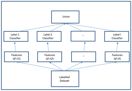
Figure 1.
View as an Ensemble.
3.6. Geometric Interpretation
Based on the Vector Space Model, we can interpret that each feature of a document is represented as a dimension of the feature vector.
The rfl modification considers the relationship between the features of the documents belonging to the label under classification and the features of the documents belonging to other labels, different from the l label under evaluation.
By applying the weight , it is sought that the value corresponding in the vector to the characteristic t increases when that characteristic occurs more in the set of documents labeled under l than in the rest of the labels, and in turn, that it decreases when t occurs less in l than in the rest of the labels.
The geometric interpretation is that the value in dimension t of the vector increases, that is, it moves away from the other vectors corresponding to the other labels. This is exemplified in the following graph.
Figure 2 shows how under the logic of the Vector Space Model, every time a representation is modified, depending on the label to which it will be evaluated, the texts will “move away” from each other, facilitating the search for the separating hyperplane.
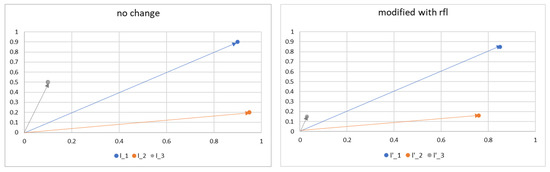
Figure 2.
Geometric interpretation.
4. Experimental Method
This section presents the classification method, the data sets, and the performance measurements of the evaluation.
4.1. Classification Method
The computational experiments considered 10 widely available data sets. Firstly, each multilabeled data set was preprocessed for conversion into single-label data sets using Binary Relevancy and Label Powerset transformations. New representations were obtained for each post-processed data set. Secondly, classification of the newly generated data sets was accomplished by means of binary machine learning techniques. Thirdly, the classification performance was analyzed. The whole procedure is graphically presented in Figure 3.
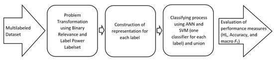
Figure 3.
Text processing flow.
4.2. Data Sets
There are many standardized data sets for the testing models; the top 10 multilabeled textual data sets are: REUTERS-21578, OHSUMED, ENRON, SLASHDOT, LANGLOG, BIBTEX, TMC, Yahoo Education, Yahoo Science, and MEDICAL. For REUTERS-21578, which is a set of news texts, a modified subset that was proposed in [30] was considered in order to be able to obtain comparative performance measures. The OHSUMED data set is a partition of the MEDLINE database, which is a library of scientific articles published in medical journals. The OHSUMED collection has also been reduced from 50,216 to 13,929 texts. This subset contains the 10 most representative categories of the original 23 categories. The Enron data set is a collection of texts created by the CALO (Cognitive Assistant that Learns and Organizes) project, containing 1702 email messages and 52 categories. Finally, the Medical data set was created by the Computational Medicine Center, 2007, for the Language Processing Challenge, 2007; it contains 978 clinical texts of radiology reports and considers 45 categories of medical codes. TMC2007 is a subset of the Aviation Safety Reporting System data set. Finally, we use real web pages linked from the “yahoo.com” domain, specifically comparing “Science” and “Education”. Table 5 presents the characteristics of the preprocessed data set.
Table 5.
Characteristics of the Preprocessed Data Set. Cardinality (Card) measures the average number of labels associated with each document. Density (Dens) is defined as the cardinality divided by the number of labels. The Diversity (Div) represents the percentage of label sets present in the set divided by the number of possible label sets. Vocabulary Size considers the volume of distinct words.
4.3. Performance Measures
Traditional evaluation measures such as the F measure, Hamming Loss, and Accuracy are useful in the case of multilabeled sets.
To describe the performance measures, the following notation was used: considering the vector … d, then each label will be relevant if , and for its part, the prediction of the classifier will be , where d is the number of documents and is the number of possible labels.
Based on the notation above, Hamming Loss is defined as in Equation (6):
where represents the difference between the labels assigned by the classifier and the actual labels. This measure seeks to measure the difference between each label that the texts actually have, with each label that the classifier assigned to said texts. The lower the value obtained, the better the performance.
Another multilabel measure is the label set precision (Accuracy), and this is defined as in Equation (7):
This average performance allowed us to measure, for each text, the correctly assigned labels. In multilabel classification, the function returns the precision of the subset. If the entire set of predicted labels for a sample strictly matches the actual set of labels, then the subset precision is 1; otherwise, it is 0. The higher the returned value, the better the performance.
The F measure, commonly used in information retrieval, is very popular in multilabeled text classification. The measure F is the harmonic mean between precision and completeness (recall). The measure F for each label was calculated as shown in Equation (8):
where Accuracy is the fraction of the predictions that are actually relevant, and recall is the fraction of actual relevance with respect to the predictions. The higher the value of F, the better the performance.
For the multilabel case, it is necessary to combine the different of each evaluation of the label. For that we use macro-, which is the average of for each label.
5. Results and Discussion
In order to compare the effects of using the function to modify the representation, we carried out different classification experiments using 10 different data sets widely worked on in the literature (Reuters, Ohsumed, Enron, Slashdot, Langdot, Bibtex, Medical, TMC2007, and Science and Education), using bin-rfl and bin-idf representations, both with the Binary Relevance and Label Powerset transformations, and with two different linear classifiers (SVM and ANN). The objective of using these linear classifiers was to evaluate the modification, independent of the classification model.
The impact of modifying the representation can be assessed using shallow learning models, which work well under conditions of limited computational complexity, as they do not require prior domain knowledge or experience to extract features from the original text. In turn, smaller data sets of the multilabel classification problem are used, which are widely known in the literature. These sets had already been preprocessed in the standard way.
Table 6, Table 7, Table 8, Table 9, Table 10 and Table 11 show the different methods and their performances in terms of the different performance measures described previously.
Table 6.
Experimental results of different transformations of the problem (PT: BR and LP), and Representations with SVM in terms of Accuracy.
Table 7.
Experimental results of different transformations of the problem (PT: BR and LP), and Representations with ANN in terms of Accuracy.
Table 8.
Experimental results of different transformations of the problem (PT: BR and LP), and Representations with SVM in terms of Hamming Loss.
Table 9.
Experimental results of different transformations of the problem (PT: BR and LP), and Representations with ANN in terms of Hamming Loss.
Table 10.
Experimental results of different transformations of the problem (PT: BR and LP), and Representations with SVM in terms of macro-.
Table 11.
Experimental results of different transformations of the problem (PT: BR and LP), and Representations with ANN in terms of macro-.
Regarding the classifiers, the results of the SVMs are at odds with those of the ANNs. Binary Relevance in general performs better than Label Powerset, unless the evaluation is in terms of Accuracy, where some LP data sets perform better than BR.
Regarding rendering, in almost all cases, the bin-rfl rendering has improvements to bin-idf. As shown in Table 6 and Table 7, an average improvement of over 15% (with SVM) and 40% (with ANN) is obtained in terms of Accuracy. Similarly, improvements of 12% in terms of Hamming Loss are obtained with ANN, as shown in Table 8 and Table 9.
In [24], the Classification Neural Networks (CNN) model was used, and it was tested in the following data sets: Enron, and Medical and Science, among others. From this, we can compare the results in terms of Hamming Loss. A value of is reported for Enron, for Medical, and for Science. In this comparison, our proposal receives a Hamming Loss value of , , and , respectively. In all three data sets, the proposal evaluated in this research is better than CNN.
Finally, as can be seen in Table 10 and Table 11, the performance improvement in terms of macro- are 40% (with SVM) and 50% (with ANN), averaged using the bin-representation rfl instead of bin-idf and the Binary Relevance transformation.
Here, it can also be mentioned that from [29], performance measures are reported using the same data sets used in this research: Science, Education, and Enron and Bixtex, comparing their PNML proposal, achieving a macro- of , , , and , respectively. In this comparison, our proposal achieves a macro- of , , , and , respectively. From the above, it is possible to appreciate that superficial learning models can deliver better results than some deep learning models, in 3 of the 10 data sets compared.
To present the impact of the function on the experimental results, Figure 4 graphically shows how, in almost all cases, the bin-rfl representation presents significant improvements in relation to bin-idf. This percentage is calculated as the ratio between the difference of the metric with the new representation and the old representation. It can be seen from the figure that the improvements, in many cases, are greater than 20%, in terms of macro-.
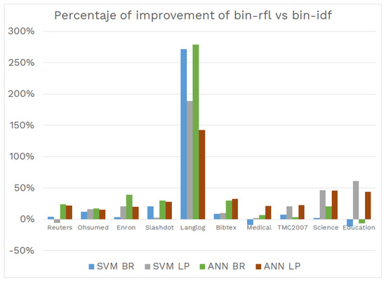
Figure 4.
Percentage performance improvement in terms of macro-.
In order to analyze the relationship between the performance improvements introduced by the function in the different evaluated metrics—Hamming Loss, Accuracy, and macro-, with the different characteristics of the sets of documents analyzed (number of labels, number of documents, number of terms in the vocabulary, cardinality, density and diversity)—a correlation analysis of the metrics and characteristics was carried out, identifying the relationships that are explained below. A correlation analysis was carried out by analyzing the output of each classifier and the input characteristics as variables. The proximity of the correlation coefficient is to +1 or −1 indicates a positive (+1) or negative (−1) correlation between variables. A positive correlation means that if the values in one matrix increase, the values in the other matrix also increase. A correlation coefficient that is closer to 0 indicates no correlation or a weak correlation.
Remember that the cardinality metric is calculated as the average number of labels that a document has, density as the cardinality divided by the total number of labels, and diversity as the percentage of label sets present in the split document set, by the number of possible label sets.
First, the relationship was analyzed in the Hamming Loss metric, as shown in Figure 5. In this analysis, it was possible to identify an inverse correlation between the use of SVM with the transformation of the problem with the number of labels and with the diversity of labels. In addition, a direct correlation exists between this transformation of the problem and the number of documents, vocabulary size, label density, and label diversity. Likewise, it is possible to appreciate that there is an inverse correlation between the use of ANN with the transformation of the problem with the cardinality and diversity of the document set.
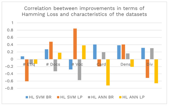
Figure 5.
Correlation between performance improvements in terms of and the different characteristics of the data set (number of labels, number of documents, number of vocabulary terms, cardinality, density, and diversity).
Secondly, the relationship in the Accuracy metric is analyzed, which, as shown in Figure 6, presents an inverse correlation with the number of documents and a direct correlation with the diversity of labels. It can also be seen that using SVM with the transformation obtains better performances with fewer documents, a smaller vocabulary size, and a lower value of the label cardinality and density measures.
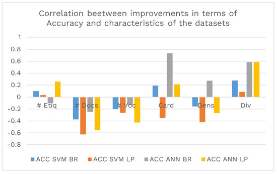
Figure 6.
Correlation between performance improvements in terms of and the different characteristics of the data set (number of labels, number of documents, number of vocabulary terms, cardinality, density, and diversity).
Third, as shown in Figure 7, the relationship in the macro- metric with the different sets of documents was analyzed. In this performance measure. it is possible to identify a negative correlation of the two classifiers (SVM and ANN) with the two transformations of the problem (BT and LP) with the number of labels, the number of documents, and the size of the vocabulary. Likewise, a direct correlation with the cardinality, density, and diversity of labels is presented. This can be interpreted as the smaller the number of documents or the smaller the vocabulary, the greater the improvement introduced by the function. Additionally, it shows that with the greater the cardinality of labels, the diversity of labels and, to a lesser extent, the density of labels, the improvement introduced by the function is greater in the macro- measure.
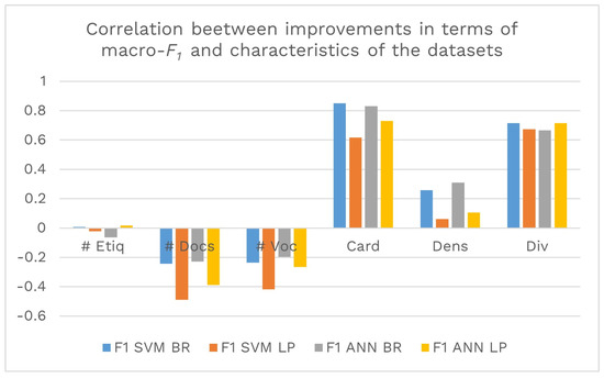
Figure 7.
Correlation between the performance improvements in terms of macro- and the different characteristics of the data set (number of labels, number of documents, number of vocabulary terms, cardinality, density, and diversity).
To evaluate the results as in [1], a test based on a two-tailed paired t-test at the 5% significance level was implemented. According to these results, the transformation of the Binary Relevance problem with ANN and bin-rfl is better than Binary Relevance with ANN and bin-idf in all measures (p = 0.0103 for Accuracy, p = 0.0491 for Hamming Loss, and p = 0.0078 for ). The p value shown in parentheses provides additional quantification of the significance level.
6. Conclusions and Future Scope
6.1. Conclusions
The growth of interest in deep learning models does not rule out the techniques and models based on shallow learning, especially when the set of training cases is smaller and the set of features is not very extensive. The “white box” versus the “black box” approaches have some advantages, especially the feasibility of working with relatively small data sets and the interpretability of the results. Issues in some fields of application are fundamental.
Classification with multiple labels is an important topic in information retrieval and machine learning, which has become more relevant in recent years. Text representation and classification have traditionally been handled using -, due to its simplicity and good performance. However, the - representation does not take into account that the examples may have different labels. The latter is very relevant in data sets with high cardinality and label diversity.
Changes in the input representation to classifiers can use knowledge about the problem, its domain, a particular label, or the category to which the document belongs. The function can be written to solve a particular problem directly and without complex problem transformations, using the information from the examples and their different labels.
In this work, we have introduced the function to build new text representations for the multilabel classification approach. This function allows for discriminating the terms that best describe a category, in contrast to other categories, thus taking advantage of the characteristics of the domain of documents that make up the corpus.
This proposal was evaluated using two different linear classifiers, Artificial Neural Networks (ANN) and Support Vector Machines (SVM), with the aim of evaluating the impact of the function on simple classifiers. In turn, the impact was evaluated on 10 different sets of texts, which correspond to medical scientific articles, journalistic documents, medical diagnostic reports, email messages, and web pages. A comparison with was made, and two transformations of the multilabeling problem were used (Binary Relevance and Label Powerset).
The performance of this function shows an improvement in almost all cases, using the Binary Relevance transformation and Support Vector Machines. Only to the extent of Hamming Loss was it better to use Label Powerset and Support Vector Machines.
The greatest impact of using the function occurs on the macro- performance metric when the data sets have fewer labels, fewer documents, and smaller vocabulary sizes. In addition, this measure improves on data sets with higher cardinalities, densities, and diversities of labels. This reflects the utility of the function on smaller data sets.
We believe that the contribution of the use of the function, when using it as a weighting factor to modify the multilabel representation, is due to a better resolution of the considered problem, since it is capable of making a better identification of the terms in the documents, which is reflected in a better performance of the classification models. From the perspective of machine learning applications and the increasing rate of their adoption in the industry, one must consider the need to develop computationally lightweight models that can be implemented under affordable technological conditions for companies of different sizes.
6.2. Future Scope
In future studies, we plan to use the function for the task of selecting features or for identifying the most significant attributes to discriminate. In addition, other representations, e.g., Part of Speech or N-grams, or based on other probability distributions, could be used to construct a label-dependent representation.
We will also take an in-depth look at the impact of the function on the performance of non-linear classifiers, such as Random Forest and Decision Tree. Previous results show important improvements in these non-linear classifiers, and the challenge is to understand how these classifiers recognize the changes caused by the function to improve their performance.
We will also use the function to process the outputs of more complex learning models—for example, with word2vec—in order to improve its performance, starting from the incorporation of information from the labels to weight the synthesized concepts.
Another line of work is to incorporate weights into the function that allow the attacking of the imbalance problem, which is very common in multilabel classification. This can be achieved by adding the number of documents for each label in relation to the total number of documents and labels as a parameter of the function.
Finally, we will use the representation to perform sentiment analysis, email classification, and other pattern recognition applications.
Author Contributions
Conceptualization, R.A.; methodology, R.A., H.A.-C. and H.A.; software, R.A.; validation, R.A., H.A.-C. and H.A.; formal analysis, R.A. and H.A.; investigation, R.A. and H.A.; resources, R.A. and H.A.; data curation, R.A.; writing — original draft preparation, R.A., H.A.-C. and H.A.; writing, R.A., H.A.-C. and H.A.; visualization, R.A.; supervision, H.A.-C. and H.A. All authors have read and agreed to the published version of the manuscript.
Funding
This research was partially funded by ANID Fondef Idea I+D ID21I10206 (2021–2023) and PUCV Grant 039.406/2021 and 039.344/2022. As well as the Applied Natural Language Processing Nucleo (NIPLNA, www.niplna.com, accessed on 8 March 2023).
Institutional Review Board Statement
Not applicable.
Informed Consent Statement
Not applicable.
Data Availability Statement
Data is contained within the article.
Conflicts of Interest
The authors declare that they have no known competing financial interest or personal relationships that could have appeared to influence the work reported in this paper.
References
- Alfaro, R.; Allende, H. Text Representation in Multi-label Classification: Two New Input Representations. In Adaptive and Natural Computing Algorithms; Dobnikar, A., Lotric, U., Ster, B., Eds.; ICANNGA: Ljubljana, Slovenia, 2011. [Google Scholar]
- Alfaro, R.; Allende, H. Clasificación de Textos Multi-etiquetados con Modelo Bernoulli Multi-variado y Representación Dependiente de la Etiqueta. Rev. Signos 2020, 53, 549–567. [Google Scholar] [CrossRef]
- Ñanculef, R.; Concha, C.; Allende, H.; Candell, D.; Moraga, C. AD-SVMs: A Light Extension of SVMs for Multicategory Classification. Int. J. Hybrid Intell. Syst. 2009, 6, 69–79. [Google Scholar] [CrossRef]
- Yang, L.; Su, H.; Zhong, C.; Meng, Z.; Luo, H.; Li, X.; Tang, Y.Y.; Lu, Y. Hyperspectral image classification using wavelet transform-based smooth ordering. Int. J. Wavelets Multiresolution Inf. Process. 2019, 17, 1950050. [Google Scholar] [CrossRef]
- Guariglia, E.; Silvestrov, S. Fractional-Wavelet Analysis of Positive definite Distributions and Wavelets on D′ (ℂ). In Proceedings of the Engineering Mathematics II; Silvestrov, S., Rančić, M., Eds.; Springer: Cham, Switzerland, 2016; pp. 337–353. [Google Scholar]
- Mallat, S. A theory for multiresolution signal decomposition: The wavelet representation. IEEE Trans. Pattern Anal. Mach. Intell. 1989, 11, 674–693. [Google Scholar] [CrossRef]
- Yu, B.; Li, B. Fractal-like tree networks reducing the thermal conductivity. Phys. Rev. E Stat. Nonlin. Soft Matter Phys. 2006, 18, 066302. [Google Scholar] [CrossRef]
- Guariglia, E. Entropy and Fractal Antennas. Entropy 2016, 18, 84. [Google Scholar] [CrossRef]
- Berry, M.V.; Lewis, Z.V.; Nye, J.F. On the Weierstrass-Mandelbrot fractal function. Proc. R. Soc. Lond. A Math. Phys. Sci. 1980, 370, 459–484. [Google Scholar]
- Viswanathan, P.; Chand, A. Fractal rational functions and their approximation properties. J. Approx. Theory 2014, 185, 31–50. [Google Scholar] [CrossRef]
- Li, Q.; Peng, H.; Li, J.; Xia, C.; Yang, R.; Sun, L.; Yu, P.S.; He, L. A Survey on Text Classification: From Traditional to Deep Learning. ACM Trans. Intell. Syst. Technol. 2020, 13, 31. [Google Scholar] [CrossRef]
- Maron, M.E. Automatic Indexing: An Experimental Inquiry. J. ACM 1961, 8, 404–417. [Google Scholar] [CrossRef]
- Cover, T.; Hart, P. Nearest Neighbor Pattern Classification. IEEE Trans. Inf. Theory 1967, 13, 21–27. [Google Scholar] [CrossRef]
- Joachims, T. Learning to Classify Text Using Support Vector Machines: Methods, Theory, and Algorithms; Kluwer Academic: Dordrecht, The Netherlands, 2002. [Google Scholar]
- Anthes, G. Deep learning comes of age. Commun. ACM 2013, 56, 13–15. [Google Scholar] [CrossRef]
- Severyn, A.; Moschitti, A. Learning to rank short text pairs with convolutional deep neural networks. In Proceedings of the 38th International ACM SIGIR Conference on Research and Development in Information Retrieval, Santiago, Chile, 9–13 August 2015; pp. 373–382. [Google Scholar]
- Samir, K.; Takehisa, Y. A review on the application of deep learning in system health management. Mech. Syst. Signal Process. 2018, 107, 241–265. [Google Scholar]
- Rudin, C. Stop explaining black box machine learning models for high stakes decisions and use interpretable models instead. Nat. Mach. Intell. 2019, 1, 206–215. [Google Scholar] [CrossRef] [PubMed]
- Zeng, J.; Ustun, B.; Rudin, C. Interpretable classification models for recidivism prediction. J. R. Stat. Soc. Ser. (Stat. Soc.) 2016, 180, 689–722. [Google Scholar] [CrossRef]
- Sebastiani, F. Machine learning in automated text categorization. ACM Comput. Surv. 2002, 34, 1–473. [Google Scholar] [CrossRef]
- Tsoumakas, G.; Katakis, I. Multi label classification: An overview. Int. J. Data Wareh. Min. 2007, 3, 1–13. [Google Scholar] [CrossRef]
- Lee, S.; Jiang, J. Multilabel text categorization based on fuzzy relevance clustering. Fuzzy Syst. IEEE Trans. 2014, 22, 1457–1471. [Google Scholar] [CrossRef]
- Nam, J.; Kim, J.; Mencía, E.; Gurevych, I.; Fürnkranz, J. Large-scale multi-label text classification -Revisiting Neural Networks. In Machine Learning and Knowledge Discovery in Databases; Springer: Berlin/Heidelberg, Germany, 2014; pp. 437–452. [Google Scholar]
- Giunchiglia, E.; Lukasiewicz, T. Multi-Label Classification Neural Networks with Hard Logical Constraints. arXiv 2021, arXiv:2103.13427v1. [Google Scholar] [CrossRef]
- Devlin, J.; Chang, M.W.; Lee, K.; Toutanova, K. Bert: Pre-training of deep bidirectional transformers for language understanding. arXiv 2018, arXiv:1810.04805. [Google Scholar]
- Pal, A.; Selvakumar, M.; Sankarasubbu, M. MAGNET: Multi-Label Text Classification using Attention-based Graph Neural Network. arXiv 2020, arXiv:2003.11644. [Google Scholar]
- Murawaki, Y. Global model for hierarchical multi-label text classification. In Proceedings of the International Joint Conference on Natural Language Processing, Guangzhou, China, 24–26 March 2013; pp. 46–54. [Google Scholar]
- Liu, J.; Chang, W.C.; Wu, Y.; Yang, Y. Deep learning for extreme multi-label text classification. In Proceedings of the 40th International ACM SIGIR Conference on Research and Development in Information Retrieval (SIGIR ’17), Tokyo, Japan, 7–11 August 2017; pp. 115–124. [Google Scholar]
- Yang, Z.; Han, Y.; Yu, G.; Yang, Q.; Zhang, X. Prototypical Networks for Multi-Label Learning. arXiv 2020, arXiv:1911.07203. [Google Scholar]
- Read, J.; Pfahringer, B.; Holmes, G.; Frank, E. Classifier chains for multi label classification. Mach. Learn. 2011, 85, 333–359. [Google Scholar] [CrossRef]
- Fink, E. Automatic evaluation and selection of problem-solving methods: Theory and experiments. J. Exp. Theor. Artif. Intell. 2004, 16, 73–105. [Google Scholar] [CrossRef]
- Kadhim, A.I. Term weighting for feature extraction on Twitter: A comparison between BM25 and TF-IDF. In Proceedings of the International Conference on Advanced Science and Engineering (ICOASE), Duhok, Iraq, 2–4 April 2019; pp. 124–128. [Google Scholar]
- Chatterjee, A.; Gupta, U.; Chinnakotla, M.K.; Srikanth, R.; Galley, M.; Agrawal, P. Understanding emotions in text using deep learning and Big Data. Comput. Hum. Behav. 2019, 93, 309–317. [Google Scholar] [CrossRef]
- Keikha, M.; Razavian, N.; Oroumchian, F.; Razi, H.S. Document Representation and Quality of Text: An Analysis. En Survey of Text Mining II: Clustering, Classification, and Retrieval; Springer: Berlin/Heidelberg, Germany, 2008; pp. 135–168. [Google Scholar]
- Manning, C.; Schütze, H. Foundations of statistical natural language Processing; The MIT Press: Cambridge, MA, USA, 1999. [Google Scholar]
- McCallum, A.; Nigam, K. A comparison of event models for naive bayes text classification. In Proceedings of the AAAI-98 Workshop on Learning for Text Categorization, Madison, WI, USA, 26–27 July 1998; pp. 41–48. [Google Scholar]
- Leopold, E.; Kindermann, J. Text categorization with support vector machines. How to represent texts in input space? Mach. Learn. 2002, 46, 423–444. [Google Scholar] [CrossRef]
- Lan, M.; Tan, C.L.; Su, J.; Lu, Y. Supervised and traditional term weighting methods for automatic text categorization. IEEE Trans. Pattern Anal. Mach. Intell. 2009, 31, 721–735. [Google Scholar] [CrossRef]
- Salton, G.; Buckley, C. Term-weighting approaches in automatic text retrieval. Inf. Process. Manag. Int. J. 1988, 24, 513–523. [Google Scholar] [CrossRef]
- Kowsari, K.; Jafari, M.K.; Heidarysafa, M.; Mendu, S.; Barnes, L.; Brown, D. Text classification algorithms: A survey. Information 2019, 10, 150. [Google Scholar] [CrossRef]
- Valle, C. Ensemble Learning with Locally Coupled Learners. Ph.D. Thesis, Universidad Técnica Federico Santa Maria, Valparaiso, Chile, 2014. [Google Scholar]
- Rokach, L. Taxonomy for characterizing ensemble methods in classification tasks: A review and annotated bibliography. Comput. Stat. Data Anal. 2009, 53, 4046–4072. [Google Scholar] [CrossRef]
Disclaimer/Publisher’s Note: The statements, opinions and data contained in all publications are solely those of the individual author(s) and contributor(s) and not of MDPI and/or the editor(s). MDPI and/or the editor(s) disclaim responsibility for any injury to people or property resulting from any ideas, methods, instructions or products referred to in the content. |
© 2023 by the authors. Licensee MDPI, Basel, Switzerland. This article is an open access article distributed under the terms and conditions of the Creative Commons Attribution (CC BY) license (https://creativecommons.org/licenses/by/4.0/).