Abstract
Sleep stage classification is of great importance in sleep analysis, which provides information for the diagnosis and monitoring of sleep-related conditions. To accurately analyze sleep structure under comfortable conditions, many studies have applied deep learning to sleep staging based on single-lead electrocardiograms (ECGs). However, there is still great room for improvement in inter-subject classification. In this paper, we propose an end-to-end, multi-scale, subject-adaptive network that improves the performance of the model according to the model architecture, training method, and loss calculation. In our investigation, a multi-scale residual feature encoder extracted various details to support the feature extraction of single-lead ECGs in different situations. After taking the domain shift caused by individual differences and acquisition conditions into consideration, we introduced a domain-aligning layer to confuse the domain. Moreover, to enhance the performance of the model, the multi-class focal loss was used to reduce the negative impact of class imbalance on the learning of the model, and the loss of sequence prediction was added to the classification task to assist the model in judging sleep stages. The model was evaluated on the public test datasets SHHS2, SHHS1, and MESA, and we obtained mean accuracies (Kappa) of 0.849 (0.837), 0.827 (0.790), and 0.868 (0.840) for awake/light sleep/deep sleep/REM stage classification, which confirms that this is an improved solution compared to the baseline. The model also performed outstandingly in cross-dataset testing. Hence, this article makes valuable contributions toward improving the reliability of sleep staging.
1. Introduction
1.1. Background
Sleep status is an important indicator for evaluating human health. During deep sleep, the body can recover through metabolism, which is the main way in which the human body eliminates physical fatigue. Sleep disorders are closely related to many health problems [1], such as memory loss, a lack of energy, and low immunity. Therefore, sleep monitoring and evaluation are of great value to solve sleep-related conditions in medical fields [2].
Human sleep is mainly divided into three stages, the awake stage, the rapid eye movement stage (REM), and the non-rapid eye movement stage (NREM), when considered according to the differences in electroencephalograms (EEGs) [3]. Among them, the NREM stage can be divided into four stages, of which stage 1 and stage 2 are light sleep, while stage 3 and stage 4 are deep sleep. A sleep stage is inferred from the analysis of 30 s of data [4]. Traditional sleep staging mainly uses EEGs, electrooculograms (EOGs), and electromyography (EMG) for analysis. This is termed the polysomnography method (PSG), which is complicated and costly. During the test, multiple electrodes need to be attached to subjects, which causes discomfort [5,6]. Furthermore, although sleep should be monitored in a free-living environment and in a non-obtrusive way to ensure that the sleep captured is as representative of typical sleep as possible, in order to understand the role of sleep in health and illness [7], generally, PSG can only be conducted in a specific laboratory or hospital. In recent years, there has been a significant expansion in the development and use of low-cost [8,9], wearable sleep detection systems to study sleep architectures in free-living conditions among individuals at a population level [10,11,12]. Electrocardiograms (ECGs) are one of the most commonly used diagnostic tools in medicine and healthcare, and sleep detection systems allow individuals to be monitored by ECG signals from a wearable device, which has little effect on sleep monitoring under comfortable conditions. This potential to obtain sleep information from a single-lead ECG is of great significance.
1.2. Related Work
With the development of deep learning, there have been many studies on sleep staging based on ECGs [13]. Wei et al. (2018) extracted features of ECGs, which were input into a four-layer DNN model to distinguish the awake, REM, and NREM sleep stages. The results showed an accuracy of 77%, and Cohen’s Kappa coefficient was around 0.56 on the MIT-BIH Polysomnographic Database [14]. Qiao Li et al. (2018) combined convolutional neural networks (CNNs) and a support vector machine to improve the performance of sleep staging in terms of awake, light sleep, deep sleep, and REM based on cardiopulmonary coupling (CRC) spectrograms. The work was ten-fold cross-validated on the MIT-BIH Polysomnographic Database and achieved an accuracy of 75.4%, while Cohen’s Kappa coefficient was 0.54 [15]. Sun H. et al. (2019) developed a CNN in combination with a long short-term memory (LSTM) recurrent neural network to stage sleep from an ECG and respiratory signals. Their networks were trained and evaluated on a large clinical dataset and achieved the best performance compared to other models for staging in terms of five sleep stages (Cohen’s Kappa 0.585, 95% CI ± 0.017) and discriminating awake vs. REM vs. NREM (Cohen’s Kappa 0.760, 95% CI ± 0.019) [16]. Radha M et al. (2019) used LSTM to classify the sleep stages into four classes (wake, REM, N1/N2, and N3) based on heart rate variability (HRV) derived from an ECG. The Cohen’s Kappa for the model was 0.61 ± 0.15, and the accuracy was 77.00 ± 8.90% across the Siesta database [17]. Sridhar N et al. (2020) achieved an accuracy of 0.77 and an overall Kappa of 0.66 for four-sleep-stage classification using a deep neural network based on the instantaneous heart rate (IHR) time series, as extracted from a single-lead ECG [18].
Generally, deep learning can automatically classify sleep based on manual features and ECG-derived signals into between two and four stages. Although the current methods have achieved good performance, there is still great room for improvement in inter-subject classification. An algorithm’s generalization is restricted in inter-subject sleep staging [19] since ECG results are subject to individual differences, as charted in the field of identity recognition [20,21]. Additionally, both imbalances between the awake, REM, light sleep, and deep sleep classes during training and the limited amount of information that can be obtained from single-lead ECGs negatively impact classification.
1.3. Contributions
Extending on our previous work [22], in this article, to extract more detailed information from a single-lead ECG signal and thereby improve its sleep-staging performance, we developed a domain-based adaptive classification model based on a multi-scale residual network. A branch structure was added to the residual module of the model to construct an extraction module and thus achieve the multi-scale extraction and fusion of spatial features through detailed information gained from a single-lead ECG. To solve the class imbalance, we applied multi-class focal loss to learn hard samples by the factor, and we applied different weights for each of the classes. Meanwhile, the loss of sequence prediction was used as additional supervised information according to the relevance of the state transition in the sleep structure. The main contributions of this work are as follows:
- (1)
- An end-to-end multi-scale adaptive network is presented to classify sleep stages into four classes in an inter-subject mode based on a single-lead ECG.
- (2)
- The multi-class focal loss was combined with the loss of sequence prediction to improve the performance of sleep staging.
- (3)
- The proposed method was evaluated on public datasets and achieves state-of-the-art performance in terms of accuracy and Cohen’s Kappa for inter-subject sleep staging.
The rest of this article is organized as follows: Section 2 introduces the method of the multi-scale residual adaptive network proposed in this paper. Section 3 describes the public dataset used in this paper and the results of the experiments. Section 4 discusses the performance of the proposed method in the cross-dataset mode and the comparison results of different losses. Section 5 provides the conclusions of this paper.
2. Materials and Methods
In essence, with the given training set and test set , which are sampled from joint distributions and , respectively, the goal is to predict the labels of the test set when , which leads to the poor generalization of the model. and are the numbers of sequences in the training set and test set. To improve the performance of classification, our proposed method, a multi-scale, inter-subject network, tries to extract multi-scale, detailed information for feature representation and to transform the feature space into a new one where through mapping function to reduce domain shift. In addition, both and have the problem of class imbalance. The process of domain adaptation with multi-class focal loss is to learn ‘hard’ samples. To improve the predictive ability of the model, we also introduce historical information , which uses the previous 30 s sequence to predict the current state as a type of additional supervision information, where denotes the current stage. An overview of the proposed method to optimize the above objectives is shown in Figure 1, which contains three steps. The process can be summarized as follows:
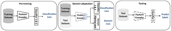
Figure 1.
An overview of our proposed domain-based, adaptive, multi-scale network for sleep stage classification. First, the model is pre-trained on the training set. Classifier 1 makes predictions based on the current sequence, while Classifier 2 makes predictions based on the previous 30 s sequence. Next, the domain-aligning layer is utilized to adjust the high-level part of the feature encoder such that the domain gap between the training set and test set can be reduced during the process of classification. Finally, the test dataset is mapped with the adjusted feature encoder to the shared feature space and classified by Classifier 1. Dashed lines indicate fixed network parameters. The blue area indicates the part that needs to be adjusted.
Pre-training: The multi-scale residual feature encoder is pre-trained by the training set to be fine-tuned in the next step for domain adaptation. There are two classifiers combined to predict the sleep stage. One is updated by the multi-class focal loss to solve the class imbalance, and the other is updated by the supervised information from the previous 30 s ECG to predict the current sleep stage.
Domain adaptation (DA): Maximum mean discrepancy (MMD) is introduced to the domain aligning layer to make the feature distributions of the training set and the test set confused during cross-iterative training.
Testing: The adjusted feature encoder and Classifier 1 are frozen to predict the sleep stages of the test set. The model is evaluated by the accuracy and Cohen’s Kappa metric (CK).
2.1. Pre-Training
For pre-training, the proposed model is mainly built on a feature encoder and two classifiers. The feature encoder contains three multi-scale residual blocks and one bidirectional gated recurrent unit (GRU) layer whose cell size is set to 64 [23,24].
The multi-scale residual block proposed in the paper contains four branches of convolutional processing, which includes convolution layers followed by a LeakyRelu [25] activation layer to transform weighted values non-linearly, as shown in Figure 2. The block uses different sizes of convolutional kernels to extract the spatial features of single-lead ECG whose kernel sizes are 1, 5, 11, and 21, respectively. Among them, the convolutional kernel with a size of 1 aims to increase or decrease the dimensions of the input signal to maintain the same number of channels as other convolutional branches. The multi-scale residual module can be expressed as
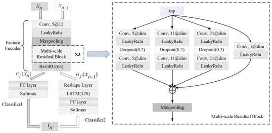
Figure 2.
The architecture of the pre-training model. and represent the current ECG sequence and the previous 30 s ECG sequence, respectively. is the prediction of the current 30 s sleep stage. “X3” means 3 multi-scale residual blocks. The block is described in the dashed box, where “5@dim” in the convolution layer indicates kernel size 5 and “dim” kernels where “dim” is different for different blocks.
In the formula, and are the input and output of the -th multi-scale residual block, respectively; is the dimension transformation function of the input signal; and is the weight of the kernel with a size of 1. is the residual mapping where represents the different scales of residual branches, and is the number of kernel channels.
For a deeper multi-scale residual block, can be expressed as
For the deeper layer in the multi-scale residual network, the shallow information and the multi-scale residual information can be directly transferred to the deeper layers to provide more detailed features.
For the residual networks [26] that have different convolutional scales, taking MESA as an example, the feature map of the first convolutional layer whose channel is set to 12 in the first residual block is shown in Figure 3. The details extracted by the convolutional kernels with scales of 5, 11, and 21 are obviously different [27]. The kernel with a scale of 5 pays more attention to high-frequency information, while the kernel with a scale of 21 pays more attention to low-frequency information. The multi-scale residual block integrates the information at these different scales through the residual structure, which not only provides more spatial information for classification but also increases the robustness of the changes in ECG.
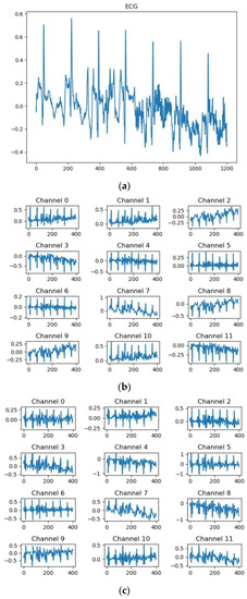
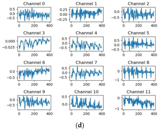
Figure 3.
The MESA’s visual feature map of the first convolutional layer for the different residual modules whose kernel size is 5 samples, 11 samples, and 21 samples, respectively. (a) A random ECG sequence for MESA, (b) feature maps extracted by residual modules whose kernel size is 5, (c) feature maps extracted by residual modules whose kernel size is 11, and (d) feature maps extracted by residual modules whose kernel size is 21.
After this, the features that are extracted by the feature encoder are flattened and sent to the first classifier, which contains a dense layer to output the probability of classes via the softmax function. An additional branch of the model seeks to use the previous 30 s ECG to predict the current sleep stage. The information from the previous stage is classified by the second classifier, which includes a reshape layer, an LSTM layer, and a dense layer. The units of the LSTM are set to 128.
However, there is the problem of class imbalance, as the different sleep stages occupy different proportions in the structure of sleep throughout the night [28]. A random sample of 100 sleep records from a related dataset was used to count the number of segments in each sleep stage, as shown in Table 1. The sample sizes for the deep sleep stage and REM are larger compared to the wake and light sleep stages.

Table 1.
The sequence number of each class of 100 random sleep records in each public dataset.
To avoid the model overfitting the head classes that have a large number of samples and ignoring the tail classes, the multi-class focal loss is used to balance the contributions of different classes. The loss function formula is as follows:
The model is supervised by the labels and prediction results of samples whose batch size is set to , and the number of classes is . The weight of class is set based on the proportion of the corresponding class to the total samples. According to the work of Lin et al. (2017) [29], the factor is set to 2 in this paper.
The transition of sleep states is correlated with timing [30]. For example, the wake stage can enter the REM stage or the NREM light sleep stage but cannot transfer to the NREM deep sleep stage directly. Inspired by this, in the process of supervised sleep stage classification, time-series historical information is added as additional information. We used historical 30 s ECG data to predict the sleep stage of the current period via LSTM. The output is then activated through the fully connected layer, the value of which is optimized by the cross-entropy loss:
Finally, the total loss of the pre-trained model is the combination of and with a weight , which is optimized by the supervised information:
2.2. Domain Adaptation
Due to individual differences, the distribution gap among subjects leads to the poor generalization ability of the pre-training model on the test set. In this part, we combine the pre-trained feature encoder, classifiers, and domain alignment layer to improve the performance of the model during testing, as shown in Figure 4.
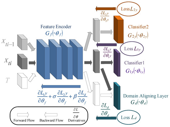
Figure 4.
The architecture of the deep adaptation network used in this paper. Different colored arrows indicate the data flow and backpropagation of different branches.
For the adjustment of the feature encoder, the last two multi-scale residual blocks are fine-tuned to adjust to a new domain, which not only solves the problem of domain shift but also reduces the number of parameters for fine-tuning. For the domain alignment layer, the MMD is used to measure the distribution gap between the two domains [22]. The output of MMD is convergent as the loss of the domain alignment layer [31,32]:
where is the set of mapping functions. MMD between the distribution and the distribution is as follows:
where the distribution is mapped to the reproducing kernel Hilbert space (RKHS) by the mapping function . For ,
and are unbiased estimates of the mean.
The details of implementation are summarized in Algorithm 1. Firstly, we freeze the domain alignment layer and update the feature encoder and classifiers by minimizing total loss L, which is defined as follows:
are the weights among the three types of loss.
Then, the domain alignment layer is updated by minimizing while the feature encoder and classifiers are frozen. The model weights are gradually adjusted in the cross-iterative process to learn the inter-subject sleep staging task.
| Algorithm 1: The Domain Adaptation Supervised Training Process. | |
| Input: | Labeled training set at time , labeled training set at time to predict sleep stages at time unlabeled test set , feature encoder with parameters , classifier with parameters , classifier with parameters , domain aligning layer with parameters , learning rate , and batch size . |
| for the number of training iterations do | |
| Sample a mini-batch of training set . Concatenate and as , sample weights . Split embedding vector to and , which is generated by when is input into the feature encoder. Freeze , update , and : Freeze , and , update : | |
| end for | |
3. Experiments
3.1. Dataset and Preprocessing
In this paper, we used the Sleep Heart Health Study Visit (SHHS1, SHHS2) [33,34], the Multi-Ethnic Study of Atherosclerosis (MESA) [35,36], and the MIT-BIH Polysomnographic Database (SLPDB) [37,38] for training and testing, which involve subjects with coronary heart disease, sleep-disordered breathing, and other diseases. Due to the different sampling rates among datasets, the single-lead ECG was resampled to a target sample rate, which was set to 250 Hz. Considering that the full datasets are too large, one hundred subjects were sampled randomly from each dataset every time according to the setting in [39], of which seventy subjects were used for training and the rest were used for testing. The results are the average of 10 runs for 100 subjects that were sampled randomly from the datasets each time. The model with an initial learning rate of 0.001 was trained on the batch of size 128 and evaluated 10 times.
3.2. Results
We tested different deep learning models in two modes, namely, inner-subject and inter-subject, to verify the domain differences in subjects. Inner-subject mode means that the dataset is divided into the training set and the test set according to the samples. This means that the samples in the test set and the samples in the training set may come from the same subject. Inter-subject mode means that the dataset is divided into the training set and the test set according to the subjects—that is, the samples in the test set cannot be from the same person as the samples in the training set. Table 2 shows the comparison results of three different feature encoders under the two types of modes on three datasets, with a CNN block with bidirectional GRU (Bi-GRU), the residual module with Bi-GRU, and the multi-scale residual model with Bi-GRU. The result shows that the performance of different models on the training set tends to be the same as the performance on the test set under the inner-subject mode. Specifically, the average accuracy and the average Kappa on the test set of the three datasets are at the same level as the training set. However, in the inter-subject mode, the performance on the training set and the test set under different models is significantly different. Specifically, the evaluation results are reduced on the test set. Compared with the training set, the average rate dropped by 15%, and the average Kappa dropped by 0.25. As shown in Figure 5, the overall features of the test set before DA are different compared with the overall features of the training set, which is reflected in the features’ confusion among classes before DA, so this causes the classifier to not distinguish the classes well.
Table 2.
The accuracy and Kappa of sleep staging on datasets in inner-subject and inter-subject mode.
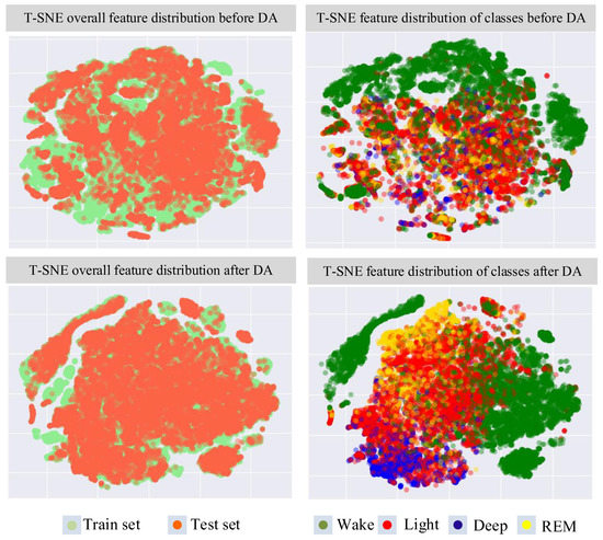
Figure 5.
T-SNE results of SHHS2′s feature distribution extracted by the CNN block module before DA and after DA.
The comparison results of the multi-scale residual module with Bi-GRU proposed in this paper on the test sets of the three datasets before and after introducing DA are shown in Table 3. The result shows that there is a significant improvement in the generalization of the model through fine-tuning and DA. Taking SHHS2 as an example, the overall distribution of the test set after DA tends to reflect the overall distribution of the training set, and the classes are more distinguishable, as shown in Figure 5. The domain loss combined with the multi-class focal loss could solve the problem of data imbalance. Meanwhile, the distribution of inter-class features is more discriminative, and the distribution of intra-class features is more concentrated. We compare the method proposed in the paper with other methods referring to the review of sleep staging based on ECGs [40,41]. The results are shown in Table 4. The proposed method achieves a state-of-the-art solution for sleep staging, which is only sensed through ECG signals. In particular, the proposed method shows a great improvement in the precision of REM and deep sleep compared with other methods. Moreover, the performance of the proposed multi-scale residual module also exceeds that of other feature encoder structures, as shown in Table 5. From the performance of the three datasets on the three different residual module models, the test set of SHHS2 obtains the best evaluation of the residual model with a kernel size of 21, and SHHS1 and MESA obtain the best evaluation of the residual model with a kernel size of 11. It can be seen that ECGs collected in different environments behave differently under different scales of convolution kernels, whose feature maps are shown in Figure 3. The multi-scale residual network can combine detailed information at multiple scales to improve the performance and robustness of the model.
Table 3.
Results of sleep stage classification on the test sets.
Table 4.
Comparison with other sleep stage classification approaches based on ECG.
Table 5.
Comparison of sleep staging with different feature extractors.
For the performance of the model on each class, as shown in Figure 6, the confusion matrix on the three test sets shows that introducing the domain alignment improves the performance of the model on each class, especially in terms of deep sleep and REM. In addition, the sensitivity of the four classes (wake, REM, light sleep, deep sleep) on SHHS2, SHHS1, and MESA before DA is (77.4%, 14.5%, 50.3%, 13.2%), (84.8%, 20.5%, 49.7%, 24.7%), and (70.0%, 12.2%, 56.8%, 12.6%), respectively, while their sensitivity after DA is (98.0%, 69.7%, 86.7%, 69.3%), (97.5%, 73.0%, 79.4%, 72.0%), and (97.3%, 69.5%, 81.2%, 59.3%), respectively. Before DA, deep sleep and REM are difficult to distinguish because the model can easily overlearn on the other two classes, which are wake and light sleep, and ignore the experience of these two classes. Meanwhile, the domain difference leads the class experience learned by the model from the training set to apply to the test set with deviation. In the process of domain alignment, to reduce the distribution difference between the training set and the test set, the multi-class focal loss uses weights and the factor to increase the error loss of hard samples from different classes. When the prediction probability of difficult samples is biased toward other error classes, their loss value is much larger than the value calculated using the cross-entropy loss function, which causes the model to pay more attention to the samples that are difficult to learn. Therefore, the model learns the information on deep sleep and REM better with the help of domain alignment based on MMD with the multi-class focal loss.
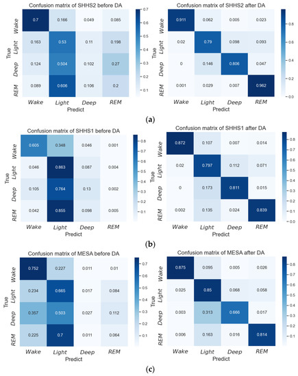
Figure 6.
Confusion matrix of inter-subject sleep staging before and after domain adaptation based on the proposed network. (a) Confusion matrix for SHHS2, (b) confusion matrix for SHHS1, and (c) confusion matrix for MESA.
There are some subjects in the test set whose results are much higher or far lower than the average, as shown in Figure 7, depending on the matching degree between the class distribution of these subjects and the classifier. For some subjects whose feature distribution is too far from the feature distribution of the training set, the adjustment effect of features after DA is limited, which leads to the situation in which the prediction performance of these subjects is far below the average level.
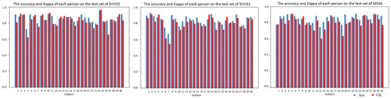
Figure 7.
An example of the accuracy (ACC) and Kappa (CK) of each subject in the test sets.
4. Discussion
In this paper, we propose a model structure, training method, and loss calculation to improve the generalization of the model. The multi-scale residual module extracts multi-scale detailed information to enhance the representation ability of the feature encoder. Multi-class focal loss with the additional classification loss that computes the loss between the prediction stages using the previous 30 s ECG and true labels solves the inadequate learning of the model caused by class imbalance and provides the learning of sleep stage transitions based on the previous period of ECG. Because the model’s experience learned on the training set is biased on the test set due to subject-specific problems [43] between the training set and the test set, we implemented domain adaptation via the iterative optimization of MMD and classification losses to improve the generalization on the test set [22]. In the above results, we have verified that the proposed method has outstanding performance on subject-specific sleep staging in the three datasets. In this part, we will discuss the test results of the proposed method across datasets and analyze the impact of different loss calculations on the model’s performance, which aims to verify that the contributions have a key effect on the model’s performance.
The model was trained on a dataset and then tested on another dataset to obtain the cross-dataset evaluation results. We tested a total of four cases, namely SHHS1 to MESA, SHHS2 to MESA, SHHS2 to SLPDB, and SHHS2 to SHHS1, as shown in Table 6. The table shows that both the accuracy rate and Kappa achieve a significant improvement across datasets compared to pre-DA and post-DA. We used different datasets (source domain) as the training set and tested the same dataset (target domain), which led to different results. For example, when SHHS1 and SHHS2 were used as the training set to train the model, respectively, the accuracy (Kappa) of MESA is 0.851(0.803) and 0.857(0.809) after adjusting the distribution. This may be related to the degree of distribution difference between different datasets, resulting from the collection environment and operation. According to the results in Table 3, the test result of MESA is 0.868 (0.840), which exceeds the result in the cross-dataset mode, which supports the notion that different acquisition conditions may also cause data distribution. Table 5 also shows the results of different feature encoders in the cross-dataset test. The proposed multi-scale residual module outperforms other feature encoders. The information at multiple scales provided by the multi-scale residual module can promote the performance of the model, whether it is on the data or across the data. When the training set comes from SHHS2, and the test set comes from SLPDB, the confusion matrix under different feature encoders is as shown in Figure 8. The multi-scale residual module achieves the highest accuracy for wake and REM. However, the accuracy for light sleep is the highest on the CNN block module, and the accuracy for deep sleep is the highest on the residual module with a kernel size of 11. However, the multi-scale residual module has the best overall performance in each class.
Table 6.
Accuracy and Kappa of sleep staging across datasets.
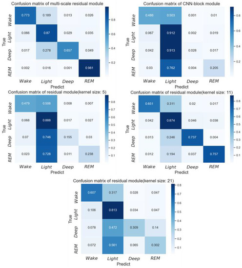
Figure 8.
Confusion matrix of the subject-specific sleep stage classification under the cross-dataset test when the training set comes from SHHS2, and the test set comes from SLPDB.
We compared the multi-class focal loss (MF) and the additional loss of sequence prediction with the cross-entropy loss (CE) to discuss the role of the proposed loss in training and domain adaptation, as shown in Table 7. We set the classifier loss to CE, MF, and MF with the additional loss, which computes the loss between the prediction based on the previous 30 s ECG and ground truth, respectively. For domain alignment, the performance of the model whose classifier uses MF far exceeds the performance of the model whose classifier uses CE. The problem of class imbalance causes the model to overfit for the head class with a large sample size. It is difficult to learn the true distribution of the samples, which affects the effect of domain adaptation. While MF causes the model to pay more attention to the tail class, it helps the model to learn the overall feature distribution better during domain adaptation. Moreover, the additional loss of sequence prediction plays a role in the improvement in accuracy and Kappa. From the comparison of the results in the table, predicting the current sleep stage based on the previous 30 s ECG provides information about the state transition to assist the model in predicting sleep stages more accurately.
Table 7.
The comparison results of different loss computation.
5. Conclusions
In this paper, a domain-based adaptive multi-scale network was proposed to improve subject-specific sleep staging based on a single-lead ECG. We presented a multi-scale residual feature encoder to extract various details, which supports the model to deal with the feature extraction of single-lead ECGs in different situations to improve the test results. Taking the domain shift caused by individual differences and acquisition conditions into consideration, we utilized MMD to optimize the feature encoder so that the features from the confused domain were obtained to make the task of sleep stage classification more generalized. In addition, to enhance the performance of the model, the multi-class focal loss was used to reduce the negative impact of class imbalance on the learning of the model, and the loss of sequence prediction was added to the classification task to assist the model in the judgment of sleep staging. Finally, the methods achieved excellent performance in terms of accuracy and Cohen’s Kappa in the three public datasets and four types of cross-dataset modes. Hence, for sleep monitoring, this approach, which outperforms the state-of-the-art solutions based on single-lead ECGs, makes contributions to the analysis of the subjects’ sleep structures under comfortable conditions.
Although the overall performance of the proposed model on the test sets is excellent, there are limitations in its robustness to different subjects. For subjects whose feature distribution is too far from the distribution of the training set, the aligning effect of domain adaptation is limited, resulting in significantly below-average accuracy of sleep staging for these subjects. The question of how to improve the prediction accuracy of the model for the sleep staging of these people so that the model can adapt to extreme distribution gaps will become a future task, seeking to make the methods of sleep staging more robust. It is a major challenge to apply the proposed method to sleep monitoring based on ECGs or other single physiological signals on wearable devices that are comfortable and portable for users.
Author Contributions
Conceptualization, Z.Z. and M.T.; methodology, Z.Z.; software, M.T.; validation, Z.Z. and M.T.; formal analysis, Z.Z. and M.T.; investigation, Z.Z. and M.T.; writing—original draft preparation, M.T.; writing—review and editing, Z.Z.; visualization, Z.Z. and M.T.; supervision, Z.Z; project administration, Z.Z.; funding acquisition, Z.Z. All authors have read and agreed to the published version of the manuscript.
Funding
This work was funded by the CGYMS Innovation Fund (2019-ZTKJ-0202).
Institutional Review Board Statement
Not applicable.
Informed Consent Statement
Not applicable.
Data Availability Statement
Not applicable.
Acknowledgments
The authors thank the editors and anonymous reviewers for their constructive suggestions.
Conflicts of Interest
The authors declare that they have no known competing financial interest or personal relationships that could have appeared to influence the work reported in this paper.
References
- Roux, F.; D’Ambrosio, C.; Mohsenin, V. Iconography: Sleep-related breathing disorders and cardiovascular disease. Am. J. Med. 2000, 108, 396–402. [Google Scholar] [CrossRef] [PubMed]
- Feige, B.; Al-Shajlawi, A.N.; Nissen, C.; Voderholzer, U.; Hornyak, M.; Spiegelhalder, K.; Kloepfer, C.; Perlis, M.; Riemann, D. Does REM sleep contribute to subjective wake time in primary insomnia? A comparison of polysomnographic and subjective sleep in 100 patients. J. Sleep Res. 2008, 17, 180–190. [Google Scholar] [CrossRef] [PubMed]
- Aserinsky, E.; Kleitman, N. Regularly occurring periods of eye motility and concomitant phenomena during sleep. Science 1953, 118, 273–274. [Google Scholar] [CrossRef] [PubMed]
- Rechtschaffen, A.; Kales, A. A Manual of Standardized Terminology, Techniques and Scoring System for Sleep Stages of Human Subjects; National Institutes of Health: Washington, DC, USA, 1968.
- Perez-Pozuelo, I.; Zhai, B.; Palotti, J.; Mall, R.; Aupetit, M.; Garcia-Gomez, J.M.; Taheri, S.; Guan, Y.; Fernandez-Luque, L. The future of sleep health: A data-driven revolution in sleep science and medicine. NPJ Digit. Med. 2020, 3, 42. [Google Scholar] [CrossRef]
- Sierra, J.C.; Sánchez, A.I.; y Quevedo-Blasco, R. Evaluación Psicológica: Técnicas y Aplicaciones, 5th ed.; Editorial Técnica AVICAM: Granada, Spain, 2023. [Google Scholar]
- Quevedo-Blasco, R.; Diaz-Roman, A.; Quevedo-Blasco, V.J. Associations between Sleep, Depression, and Cognitive Performance in Adolescence. Eur. J. Investig. Health Psychol. Educ. 2023, 13, 501–511. [Google Scholar] [CrossRef]
- Heremans, E.R.; Phan, H.; Ansari, A.H.; Borzée, P.; Buyse, B.; Testelmans, D.; De Vos, M. Feature matching as improved transfer learning technique for wearable EEG. Biomed. Signal Process. Control. 2022, 78, 104009. [Google Scholar] [CrossRef]
- Urtnasan, E.; Park, J.U.; Joo, E.Y.; Lee, K.J. Deep Convolutional Recurrent Model for Automatic Scoring Sleep Stages Based on Single-Lead ECG Signal. Diagnostics 2022, 12, 1235. [Google Scholar] [CrossRef]
- Budig, M.; Stoohs, R.; Keiner, M. Validity of Two Consumer Multisport Activity Tracker and One Accelerometer against Polysomnography for Measuring Sleep Parameters and Vital Data in a Laboratory Setting in Sleep Patients. Sensors 2022, 22, 9540. [Google Scholar] [CrossRef]
- Erdenebayar, U.; Kim, Y.; Park, J.-U.; Lee, S.; Lee, K.J. Automatic Classification of Sleep Stage from an ECG Signal Using a Gated-Recurrent Unit. Int. J. Fuzzy Log. Intell. Syst. 2020, 20, 181–187. [Google Scholar] [CrossRef]
- Pfammatter, A.F.; Hughes, B.O.; Tucker, B.; Whitmore, H.; Spring, B.; Tasali, E. The Development of a Novel mHealth Tool for Obstructive Sleep Apnea: Tracking Continuous Positive Airway Pressure Adherence as a Percentage of Time in Bed. J. Med. Internet Res. 2022, 24, e39489. [Google Scholar] [CrossRef]
- Hong, S.; Zhou, Y.; Shang, J.; Xiao, C.; Sun, J. Opportunities and challenges of deep learning methods for electrocardiogram data: A systematic review. Comput. Biol. Med. 2020, 122, 103801. [Google Scholar] [CrossRef] [PubMed]
- Wei, R.; Zhang, X.; Wang, J.; Dang, X. The eresearch of sleep staging based on single-lead electrocardiogram and deep neural network. Biomed. Eng. Lett. 2017, 8, 87–93. [Google Scholar] [CrossRef] [PubMed]
- Li, Q.; Li, Q.; Liu, C.; Shashikumar, S.P.; Nemati, S.; Clifford, G.D. Deep learning in the cross-time frequency domain for sleep staging from a single-lead electrocardiogram. Physiol. Meas. 2018, 39, 124005. [Google Scholar] [CrossRef] [PubMed]
- Sun, H.; Ganglberger, W.; Panneerselvam, E.; Leone, M.J.; Quadri, S.A.; Goparaju, B.; Tesh, R.A.; Akeju, O.; Thomas, R.J.; Westover, M.B. Sleep Staging from Electrocardiography and Respiration with Deep Learning. Sleep 2019, 43, zsz306. [Google Scholar] [CrossRef]
- Radha, M.; Fonseca, P.; Moreau, A.; Ross, M.; Cerny, A.; Anderer, P.; Long, X.; Aarts, R.M. Sleep stage classification from heart-rate variability using long short-term memory neural networks. Sci. Rep. 2019, 9, 14149. [Google Scholar] [CrossRef]
- Sridhar, N.; Shoeb, A.; Stephens, P.; Kharbouch, A.; Shimol, D.B.; Burkart, J.; Ghoreyshi, A.; Myers, L. Deep learning for automated sleep staging using instantaneous heart rate. NPJ Digit. Med. 2020, 3, 106. [Google Scholar] [CrossRef]
- Xiao, M.; Yan, H.; Song, J.; Yang, Y.; Yang, X. Sleep stages classification based on heart rate variability and random forest. Biomed. Signal Process. Control 2013, 8, 624–633. [Google Scholar] [CrossRef]
- Zhang, Y.; Zhao, Z.; Deng, Y.; Zhang, X.; Zhang, Y. Human identification driven by deep CNN and transfer learning based on multiview feature representations of ECG. Biomed. Signal Process. Control 2021, 68, 102689. [Google Scholar] [CrossRef]
- Hong, P.L.; Hsiao, J.Y.; Chung, C.H.; Feng, Y.M.; Wu, S.C. ECG Biometric Recognition: Template-Free Approaches Based on Deep Learning. In Proceedings of the 2019 41st Annual International Conference of the IEEE Engineering in Medicine & Biology Society (EMBC), Berlin, Germany, 23–27 July 2019; IEEE: Piscataway, NJ, USA, 2019. [Google Scholar]
- Tang, M.; Zhang, Z.; He, Z.; Li, W.; Mou, X.; Du, L.; Wang, P.; Zhao, Z.; Chen, X.; Li, X.; et al. Deep adaptation network for subject-specific sleep stage classification based on a single-lead ECG. Biomed. Signal Process. Control 2022, 75, 103548. [Google Scholar] [CrossRef]
- Cho, K.; Van Merriënboer, B.; Gulcehre, C.; Bahdanau, D.; Bougares, F.; Schwenk, H.; Bengio, Y. Learning Phrase Representations using RNN Encoder-Decoder for Statistical Machine Translation. In Proceedings of the Proceedings of the 2014 Conference on Empirical Methods in Natural Language Processing (EMNLP), Doha, Qatar, 25–29 October 2014. [Google Scholar]
- Hochreiter, S.; Schmidhuber, J. Long Short-Term Memory. Neural Comput. 1997, 9, 1735–1780. [Google Scholar] [CrossRef]
- Maas, A.L.; Hannun, A.Y.; Ng, A.Y. Rectifier Nonlinearities Improve Neural Network Acoustic Models. In Proceedings of the 30th International Conference on Machine Learning, Atlanta, GA, USA, 16–21 June 2013; Volume 30, p. 3. [Google Scholar]
- He, K.; Zhang, X.; Ren, S.; Sun, J. Deep residual learning for image recognition. In Proceedings of the IEEE Conference on Computer Vision and Pattern Recognition, Las Vegas, NV, USA, 26–30 June 2016; pp. 770–778. [Google Scholar]
- Eldele, E.; Chen, Z.; Liu, C.; Wu, M.; Kwoh, C.K.; Li, X.; Guan, C. An Attention-Based Deep Learning Approach for Sleep Stage Classification with Single-Channel EEG. IEEE Trans. Neural Syst. Rehabil. Eng. 2021, 29, 809–818. [Google Scholar] [CrossRef] [PubMed]
- Dursun, M.; Gunes, S.; Ozsen, S.; Yosunkaya, S. Comparison of Artificial Immune Clustering with Fuzzy C-means Clustering in the sleep stage classification problem. In Proceedings of the International Symposium on Innovations in Intelligent Systems & Applications, Trabzon, Turkey, 2–4 July 2012; IEEE: Piscataway, NJ, USA, 2012. [Google Scholar]
- Lin, T.Y.; Goyal, P.; Girshick, R.; He, K.; Dollár, P. Focal Loss for Dense Object Detection. In Proceedings of the IEEE International Conference on Computer Vision (ICCV), Venice, Italy, 22–29 October 2017; pp. 2999–3007. [Google Scholar]
- Gretton, A.; Borgwardt, K.M.; Rasch, M.J.; Schölkopf, B.; Smola, A. A Kernel Method for the Two-Sample-Problem. In NIPS’06: Proceedings of the 19th International Conference on Neural Information Processing Systems; MIT Press: Cambridge, MA, USA, 2006; pp. 513–520. [Google Scholar]
- Aggarwal, K.; Khadanga, S.; Joty, S.R.; Kazaglis, L.; Srivastava, J. A Structured Learning Approach with Neural Conditional Random Fields for Sleep Staging. In Proceedings of the 2018 IEEE International Conference on Big Data, Seattle, WA, USA, 10–13 December 2018; IEEE: Piscataway, NJ, USA, 2018. [Google Scholar]
- Yosinski, J.; Clune, J.; Bengio, Y.; Lipson, H. How transferable are features in deep neural networks? In NIPS’14: Proceedings of the 27th International Conference on Neural Information Processing Systems; MIT Press: Cambridge, MA, USA, 2014; Volume 2, pp. 3320–3328. [Google Scholar]
- Zhang, G.Q.; Cui, L.; Mueller, R.; Tao, S.; Kim, M.; Rueschman, M.; Mariani, S.; Mobley, D.; Redline, S. The National Sleep Research Resource: Towards a sleep data commons. J. Am. Med. Inform. Assoc. 2018, 25, 1351–1358. [Google Scholar] [CrossRef] [PubMed]
- Quan, S.F.; Howard, B.V.; Iber, C.; Kiley, J.P.; Nieto, F.J.; O’Connor, G.T.; Rapoport, D.M.; Redline, S.; Robbins, J.; Samet, J.M.; et al. The Sleep Heart Health Study: Design, rationale, and methods. Sleep 1997, 20, 1077–1085. [Google Scholar]
- Bild, D.E.; Bluemke, D.A.; Burke, G.L.; Detrano, R.; Roux, A.V.D.; Folsom, A.R.; Greenland, P.; Jacobs, D.R., Jr.; Kronmal, R.; Liu, K.; et al. Multi-ethnic study of atherosclerosis: Objectives and design. Am. J. Epidemiol. 2002, 156, 871–881. [Google Scholar] [CrossRef] [PubMed]
- Chen, X.; Wang, R.; Zee, P.; Lutsey, P.L.; Javaheri, S.; Alcántara, C.; Jackson, C.L.; Williams, M.A.; Redline, S. Racial/Ethnic Differences in Sleep Disturbances: The Multi-Ethnic Study of Atherosclerosis (MESA). Sleep 2015, 38, 877–888. [Google Scholar] [CrossRef] [PubMed]
- Ichimaru, Y.; Moody, G.B. Development of the polysomnographic database on CD-ROM. Psychiatry Clin. Neurosci. 1999, 53, 175–177. [Google Scholar] [CrossRef]
- Goldberger, A.L.; Amaral, L.A.; Glass, L.; Hausdorff, J.M.; Ivanov, P.C.; Mark, R.G.; Mietus, J.E.; Moody, G.B.; Peng, C.K.; Stanley, H.E. PhysioBank, PhysioToolkit, and PhysioNet: Components of a new research resource for complex physiologic signals. Circulation 2000, 101, e215–e220. [Google Scholar] [CrossRef]
- Selvaraj, N.; Narasimhan, R. Detection of sleep apnea on a per-second basis using respiratory signals. In Proceedings of the 2013 35th Annual International Conference of the IEEE Engineering in Medicine and Biology Society (EMBC), Osaka, Japan, 3–7 July 2013; IEEE: Piscataway, NJ, USA, 2013; pp. 2124–2127. [Google Scholar]
- Imtiaz, S.A. A Systematic Review of Sensing Technologies for Wearable Sleep Staging. Sensors 2021, 21, 1562. [Google Scholar] [CrossRef]
- Lesmana, T.F.; Isa, S.M.; Surantha, N. Sleep Stage Identification Using the Combination of ELM and PSO Based on ECG Signal and HRV. In Proceedings of the 2018 3rd International Conference on Computer and Communication Systems (ICCCS), Nagoya, Japan, 27–30 April 2018; pp. 258–262. [Google Scholar]
- Li, Q.; Li, Q.; Cakmak, A.S.; Da Poian, G.; Bliwise, D.L.; Vaccarino, V.; Shah, A.J.; Clifford, G.D. Transfer learning from ECG to PPG for improved sleep staging from wrist-worn wearables. Physiol. Meas. 2021, 42, 044004. [Google Scholar] [CrossRef]
- Jia, Z.; Lin, Y.; Wang, J.; Ning, X.; He, Y.; Zhou, R.; Zhou, Y.; Lehman, L.H. Multi-View Spatial-Temporal Graph Convolutional Networks with Domain Generalization for Sleep Stage Classification. IEEE Trans. Neural Syst. Rehabil. Eng. 2021, 29, 1977–1986. [Google Scholar] [CrossRef]


Disclaimer/Publisher’s Note: The statements, opinions and data contained in all publications are solely those of the individual author(s) and contributor(s) and not of MDPI and/or the editor(s). MDPI and/or the editor(s) disclaim responsibility for any injury to people or property resulting from any ideas, methods, instructions or products referred to in the content. |
© 2023 by the authors. Licensee MDPI, Basel, Switzerland. This article is an open access article distributed under the terms and conditions of the Creative Commons Attribution (CC BY) license (https://creativecommons.org/licenses/by/4.0/).