Abstract
In order to fly safely and autonomously in complex environments, UAVs need to be able to plan their trajectories in real-time. This paper proposes an improved B-spline-based trajectory generation method that can generate safe, smooth, and kinodynamically feasible trajectories in real-time. This paper firstly introduces the principle of error upper bound of the B-spline curve and proposes a new trajectory safety assurance method; then, the loss function of trajectory is constructed based on safety, smoothness, and flight time; finally, a parameter adaptive trajectory optimization method is proposed, so that obtain the safe trajectory. Compared with the existing methods, the proposed method has two important improvements: (1) it solves the problem of overly conservative safety distance estimation at control points, improves the trajectory smoothness, and reduces the required flight time; (2) it proposes a trajectory optimization method with adaptive adjustment of safety distance parameters, which improves the quality and success rate of the planned trajectory. We validate our proposed method in simulation and real-world tasks, and the test results show that the method proposed in this paper can significantly improve the quality of the generated trajectory.
1. Introduction
Unmanned aerial vehicles (UAVs) are small in size and light in weight, so they perform an important role in military, agriculture, industry, and other fields. In order to enable UAVs to perform various tasks such as detection and tracking, it is necessary to allow them to have autonomous motion ability in complex environments. Motion planning is the core to achieving autonomous motion of UAVs.
In order to realize the autonomous motion of UAVs and other robots, researchers have proposed various motion planning methods in the past decades. In the framework of the classical motion planning method, motion planning can be divided into two parts: front-end path searching and back-end trajectory generation. The task of the front-end path-searching method is to search for a feasible path from the starting point to the target point. It can be divided into three categories: search-based, sampling-based, and learning-based. Representatives of the search-based method are Dijstra [1] and [2], which represent space as a search graph and then searches for a safe path based on the graph search method. Representatives of the sampling-based method are PRM [3] and RRT [4], which obtain feasible paths through random sampling in the state space. In recent years, deep learning and reinforcement learning are also widely used in path-planning tasks. At present, all kinds of path-searching methods can find a feasible path in real-time, but there are two problems: (1) the path is too close to obstacles, and (2) the path obtained by searching is not smooth, which is not suitable for UAVs and robots to execute. Therefore, optimizing the path through the trajectory generation method is also necessary to obtain a smooth and continuous trajectory convenient for the UAV to execute.
Researchers propose various methods to optimize the path to obtain a better trajectory. Trajectory smoothing is simple and widely used in trajectory optimization. It takes the smoothing loss item of the trajectory point and the distance from the original point as the optimization objective, obtains the smooth trajectory by solving the optimization problem, and then controls the UAV to follow the trajectory based on the control algorithm to avoid the obstacle moving to the target point. However, the trajectory smoothing method may cause the collision-free trajectory to collide with the obstacle. At the same time, because it does not consider the UAV dynamic characteristics, the trajectory obtained is not optimal.
In order to optimize the trajectory, polynomial curves are widely used in trajectory representation. We can optimize the parameters of polynomial curves to obtain the optimal trajectory. Reference [5] introduces the differential flatness property of the multi-rotor UAV; that is, the trajectory of the multi-rotor UAV can be indicated as the polynomial curve. According to the representation of obstacle and dynamic constraints, the trajectory optimization method can be divided into unconstrained, hard-constrained, and soft-constrained trajectory optimization methods.
The minimum-snap trajectory generation method [5] is representative of the unconstrained trajectory generation method. After obtaining a feasible path, it selects sub-target points in the path and then represents the trajectory as a piecewise polynomial curve passing through each sub-target point. It makes the trajectory continuous by adding continuity constraints of position, velocity, and acceleration. It then obtains the minimum-snap trajectory by solving the optimization problem to minimize the energy required to obtain the trajectory. Researchers also improved the minimum-snap method: The Closed-form [6] method proposed a trajectory optimization method for closed-form solutions so that continuity constraints do not need to be considered in the solution process, thus improving the efficiency of problem-solving. At the same time, a time allocation method was proposed to optimize the time allocation of each trajectory segment of the minimum-snap to achieve faster flight [7]. A trajectory generation method based on the Bezier curve is proposed, which can ensure the continuity of trajectory based on the position of control points, thus simplifying the problem-solving process. This kind of method does not represent obstacles as constraints, so in order to ensure trajectory safety, it is necessary to detect whether the trajectory meets the safety requirements repeatedly. This method adds new control points when a collision happens in the trajectory, so it is time-consuming to solve the problem in a complex environment and cannot meet the real-time requirements.
The hard-constrained trajectory generation method represents the obstacles as the constraint condition of the optimization problem so as to ensure the safety of the trajectory obtained by the optimization solution. This kind of method is usually divided into two steps. The first step is representing the safety corridor area based on the geometric shape. The second step is to limit the trajectory in the safety corridor area and solve the safety trajectory that will not collide with the obstacle. Reference [8] generated the safety zone based on the iterative region expansion method and proposed the sum of squares algorithm to ensure that the trajectory is within the safety zone. Reference [9] proposed a safe flight corridor generation method for a 3D environment, which can generate a safe flight corridor composed of a series of ellipsoids. Reference [10] uses a fixed-size square to represent the safe zone and obtains the safe path through the optimization method. Reference [11] proposed a safe corridor generation method based on the point cloud map, which can directly generate feasible paths based on the point cloud map without building an occupancy grid map. Reference [12] propose a motion planning algorithm based on the corridor-constrained minimum control effort trajectory optimization (MINCO) framework, which was finally evaluated on an autonomous LiDAR-navigated quadrotor UAV in wooded environments, achieving flight speeds over 13.7 m/s without any prior map of the environment or external localization facility. The trajectory generation method based on hard constraints can ensure trajectory security, but it still has two problems: first, the generation of safe corridors in a 3D environment is complex; second, the trajectory may be close to the boundary of safe corridors, and thus close to obstacles.
The soft-constrained trajectory generation method sets the distance between the trajectory and the obstacle as an optimization item and obtains a safe trajectory away from the obstacle by solving the optimization problem. Reference [13] generates executable smooth trajectories by generating discrete time trajectories and using gradient descent to minimize their smoothness and collision costs. Reference [14] constructed similar optimization terms but used a gradient-free method to solve this kind of optimization problem. This method is extended to continuous-time polynomial trajectory in reference [15]. Because the time parameterization is continuous, the differential error in the numerical calculation method is avoided, and the quadrotor motion can be represented more accurately. However, the computational complexity of the above methods is large, and the success rate is low. To solve these problems, reference [16] proposed a trajectory representation method based on B-spline, which ensures trajectory safety by pushing B-spline control points away from obstacles. Reference [17] proposed a path-planning method considering the dynamic feasibility and a security assurance method based on B-spline convex hull property, which realized the safe and reliable trajectory generation. To further improve the safety of UAVs and the efficiency of trajectory planning, reference [18] considers the observation perspective of UAVs on obstacles in the trajectory generation process to avoid the collision between UAVs and new obstacles. Reference [19] proposed an approximate gradient field calculation method without building an ESDF map, significantly reducing the trajectory generation time. Reference [20] presents an optimization-based framework for multi-copter trajectory planning subject to geometrical configuration constraints and user-defined dynamic constraints. The framework can complete various flight path optimization tasks and achieve good flight effects. This kind of method has two problems: First, its security threshold is too conservative, thus sacrificing the smoothness of the trajectory to some extent; second, the security threshold of such methods is usually set to a fixed value, resulting in poor adaptation to different scenarios.
In this paper, we propose an improved trajectory generation method based on the B-spline curve, which represents the trajectory of the UAV based on the B-spline curve, then define the optimization function composed of control points, and finally obtain the optimal trajectory by solving the optimization problem. Compared with the trajectory generation method proposed in [16,19], the method proposed in this paper makes three important improvements: Firstly, this paper proposes a trajectory generation method based on the upper-bound principle of B-spline error, which uses the upper-bound property of the error between B-spline curve and control polygon to propose a more accurate calculation method of security threshold. Compared with the existing safety threshold calculation methods based on the B-spline convex hull property, the safety threshold is reduced by 60%. Then, a trajectory optimization method with dynamic parameter adjustment is proposed, which is different from the current work in which the safety threshold is set to a fixed value. The trajectory generation method proposed in this paper dynamically adjusts the distance optimization parameters according to the smoothness of the trajectory so that the method has better adaptability in different environments. Finally, a dynamic time reallocate method is proposed to obtain a better trajectory. The effectiveness of the trajectory generation method proposed in this paper is verified through simulation and real-world tasks. The test results show that the proposed method can obtain a smoother and shorter time trajectory and achieve a good flight effect in real-world tasks.
The rest of this paper is organized as follows: Section 2 introduces the background of the paper, including the differential flatness property of multi-rotor UAV and the formal definition of the trajectory generation problem. Section 3 introduces the motion-planning method proposed in this paper, including the security guarantee method, parameter adaptive adjustment method, and time reallocate method. Section 4 introduces the experiment and experiment results. Section 5 summarizes the thesis.
2. Background
In this section, we first introduce the differential flatness property of multi-rotor UAVs and the trajectory representation method based on the differential flatness property. Afterward, the trajectory generation problem is formally defined.
2.1. Differential Flatness Principle and UAV Trajectory Representation
The multi-rotor UAV can be approximated as a 6 DoF rigid body. Hence, its state includes three-axis positions: , , and three-axis angles: pitch, row, yaw, and 18-dimensional vectors of velocity and acceleration in six states. Reference [5] proved that the multi-rotor has differential flatness. Therefore, its 18-dimensional state can be represented by the following four-dimensional vector
where is the position of the multi-rotor UAV centroid and is the yaw angle. The yaw angle needs to be planned according to the task so that the UAV trajectory can be expressed as a three-axis polynomial trajectory
where
2.2. Trajectory Generation Problem Definition
The trajectory generation problem of a multi-rotor UAV can be defined as follows: Given a state space , a free state space , an initial state and a goal region , find a path such that , and and .
3. Method
As previously described, the trajectory obtained based on the path-searching method is close to the obstacle and not smooth enough. This section introduces a trajectory generation method based on B-spline. The method proposed uses the convex hull property of the B-spline and the upper-bound property of the error between the B-spline curve and the control polygon to guarantee the dynamic feasibility and safety of the trajectory. Then we set and solve the optimization problem to obtain a smooth, safe, and dynamic feasible trajectory quickly.
3.1. B-Spline Curve and Security Guarantee Method
This section introduces the trajectory representation method based on B-spline and the convex hull property and error upper-bound property of the B-spline curve and derives the representation method of dynamic feasibility and safety of the B-spline curve based on the convex hull property.
3.1.1. B-Spline-Based Trajectory Representation
B-spline curve is a trajectory representation method that uses the position of control points as parameters to generate polynomial curve-fitting control points. Because the B-spline curve is the fitting of control points, the safety and smoothness of the trajectory can be adjusted by adjusting the control points. The following parameters determine the B-spline trajectory: (1) degree of B-spline , is the highest degree of the polynomial curve; (2) collection of control points , ; (3) knot vector , where needs to meet . The position of the B-spline at time can be expressed as
is the basic function of the B-spline curve, which can be calculated by Formula (5):
where
The derivative of the B-spline trajectory can provide the velocity and acceleration of the trajectory. The B-spline trajectory is still B-spline after the derivative. Formula (7) calculates the control points of the velocity and acceleration B-spline curve.
3.1.2. Convex Hull Property of B-Splines and Guarantee of Dynamic Feasibility
To assure that the generated trajectory meets the multi-rotor UAV dynamic limits, the velocity and acceleration obtained from trajectory derivation should not exceed the maximum value of multi-rotor UAV velocity and acceleration. This paper uses the convex hull property of the B-spline curve to make the trajectory meet this requirement.
The B-spline curve is a combination of several segmented Bezier curves. According to the convex hull property of the Bezier curve, each Bezier curve is included in the convex hull composed of its control points. Figure 1 shows the property of the convex hull of the B-spline curve. The red-dotted line is a track of the B-spline curve. The red-dotted quadrilateral formed by , , , is the control polygon of the trajectory. As shown in Figure 1, the local track of the B-spline is surrounded by its corresponding control polygon.
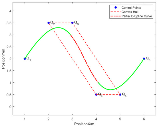
Figure 1.
The B-spline convex hull property. The solid green line is a B-spline curve. The red-dotted line is a segment of the B-spline curve. The red-dotted quadrilateral formed by , , , is the control polygon.
As described in Section 3.1.1, the velocity curve is derived from the position curve. The acceleration curve is derived from the velocity curve. Both are B-spline curves that satisfy the convex hull property. Therefore, to ensure the trajectory dynamic feasibility, that is, the trajectory speed and acceleration do not exceed the dynamic limits of the multi-rotor UAV, it is only necessary to ensure that the absolute values of the trajectory speed and acceleration control points do not exceed the maximum speed and acceleration. Therefore, B-spline control points must meet the following conditions:
By adjusting the position and knot vector of control points, the speed and acceleration control points can meet the dynamic constraints of Formula (8) so that the whole trajectory can meet the dynamic constraints of the multi-rotor UAV.
3.1.3. B-Spline Error Upper-Bound Property and Security Guarantee
In order to ensure the flight safety of multi-rotor UAVs, it is necessary to ensure that the trajectory will not collide with obstacles. This paper proposes a trajectory safety assurance method based on the upper-bound property of the error between the B-spline curve and the control polygon. Compared with the trajectory safety representation method based on the B-spline convex hull property introduced in [17], the method proposed in this paper can achieve more accurate estimation results.
The line connecting adjacent B-spline control points can be transformed into a function with time as a parameter in the domain . When , it is defined as
The maximum error between the B-spline curve and the control polygon is called the error upper bound, which is defined as shown in Formula (10).
In references [21,22], Narin et al. proved that is only related to the degree of the B-spline curve and the second-order variance of the control polygon:
In Formula (11), is the second-order variance of the control polygon, is the order of the B-spline, is a function of , which is defined as Formula (12).
is the maximum value of the second-order variance of the control polygon:
The principle of error upper bound indicates that there is an upper bound for the error between the B-spline curve and the control polygon, and it can be calculated by the second-order variance of the control polygon and the B-spline order. Based on the upper bound, this paper proposes a more accurate method for calculating the safe distance of the control point.
In Figure 2, is an arbitrary point on the B-spline curve, is the corresponding point of point on the control polygon. The distance between point and the obstacle is recorded as . The distance between and the obstacle is recorded as , and the distance between and is recorded as . According to the geometric property of the triangle,, and the upper bound of the error of the B-spline curve is recorded as , then , so to make , if , then , that is, point will not collide with the obstacle.
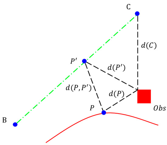
Figure 2.
The red line is a b-spline curve. The green dash line is the line connecting two control points. is an arbitrary point on the B-spline curve. B and C are the control points of the B-spline. is the corresponding point of point on the control polygon. The distance between point and the obstacle is recorded as . The distance between and the obstacle is recorded as , and the distance between and is recorded as . is the distance between the control point and the obstacle.
Mark the distance between point and point as . If point is close to point , then . According to the geometric properties of the triangle, , so only is required, that is, , then can be guaranteed to ensure , so as to ensure trajectory safety. Therefore, it is concluded that for any control point , to ensure the safety of the trajectory, it is necessary to ensure that the distance between the point and the obstacle satisfies Formula (14).
3.2. Definition of Optimization Function and Adaptive Adjustment Method
Section 3.1 discusses the necessary conditions for B-spline control points to ensure trajectory safety. Based on this conclusion, this section introduces the trajectory generation method based on optimization. This section first defines the loss function, then introduces the trajectory generation method with dynamic parameter adjustment proposed in this paper to adjust the control points, and finally introduces the time-reallocate method to generate a knot vector.
3.2.1. Optimization Function Definition
The trajectory of multi-rotor UAVs must have simultaneously the characteristics of safety, dynamic feasibility, and smoothness, so this paper defines the loss function of comprehensive safety, smoothness, and dynamic feasibility. The definition of the loss function is shown in Formula (15), which is determined by the safety loss , smoothness loss , and dynamic feasibility loss , .
where and are smoothness and collision cost; and are soft limits on velocity and acceleration; and , and trade off the smoothness, safety, and dynamic feasibility.
The trajectory safety loss is to make the distance between the trajectory control point and the obstacle meet the trajectory safety condition of Formula (14). In order to ensure trajectory safety, it is necessary to make the control point meet , where is the distance between adjacent control points. Considering the control error of a multi-rotor UAV, set the safety distance to . Therefore, the goal of the trajectory safety loss function is to make control point satisfy . For control point , its safety loss is defined as
The trajectory safety loss function is the sum of safety loss for all the control points:
The second term of the loss function is smooth loss. In this paper, the trajectory acceleration is taken as the evaluation index of the trajectory smoothing term. According to Formula (7), the size of the acceleration control point is proportional to the second derivative of the position control point, so this paper uses the square of the second derivative of the position control point to represent the smoothness of the trajectory, which is defined as Formula (18).
where , and are the control points of the B-Spline.
The last item is the flight-time loss of the trajectory. In order to ensure that the trajectory meets the dynamic feasibility, the speed control point and the acceleration control point cannot exceed the maximum speed and acceleration, that is:
Thus,
That is, the time interval between and is proportional to . By reducing the required flight time can be reduced, so
Similarly, to meet the feasibility requirements of acceleration, the trajectory needs to meet:
By reducing , can reduce and , so
Optimizing the loss function can obtain a safe, smooth, and fast trajectory suitable for the multi-rotor UAV flight.
3.2.2. Trajectory Optimization Method Based on Adaptive Adjustment
The safety loss function needs to set the safety distance threshold, which is set as a fixed value in [18,19]; that is, the trajectory needs to keep a fixed distance from the obstacle. This may cause the multi-rotor UAV to collide with obstacles if the value is set too small, and the optimization algorithm planning may fail if the value is set too large.
For the safety guarantee conditions proposed in Section 3.1.3, to ensure trajectory safety, the safety distance between the control point and the obstacle is affected by two quantities. The first is the upper bound of the error between the B-spline curve and the control polygon, and the second is the distance between the adjacent control points. The safety distance calculation formula is Formula (24).
The upper bound of the error is proportional to the second-order variance of the position control point. After the position control point is optimized according to the optimization function set in Section 3.2.1, the second-order variance of the position control point can be significantly reduced. At the same time, in the optimization process, the distance between control points also changes. Therefore, as the optimization proceeds, the safety distance required by each control point is gradually adjusted. By optimizing the trajectory, the smoothness of the trajectory gradually increases, and its safety threshold gradually decreases. Therefore, this section proposes a trajectory optimization method for the dynamic adjustment of safety distance parameters. During the optimization process, the method dynamically calculates the second-order variance of the trajectory control points and the distance between the adjacent control points, and sets the safety threshold of each control point to obtain a better-optimized trajectory while ensuring safety.
Compared with the safety assurance method based on the convex hull property described in literature [18], because its safety distance is only determined by the distance between adjacent control points, its safety threshold is a fixed threshold set in advance. Therefore, compared with this method, the proposed method can obtain a better trajectory with better comprehensive quality and adaptability in different environments.
3.2.3. Time Reallocate Method
By optimizing the objective function, a B-spline trajectory with better smoothness and dynamic feasibility can be obtained, but some of its trajectory segments may not meet the dynamic feasibility constraints, that is, some speed and acceleration control points will exceed the maximum speed and acceleration of the multi-rotor UAV. Therefore, it is necessary to adjust the original uniform knot vector to obtain a better trajectory that meets the dynamic constraints.
This paper refers to the time reallocate method in reference [18] to adjust the trajectory’s time to meet the dynamic constraints. Record the -th speed control point and acceleration control point as and , respectively. and can be calculated by Formula (25).
According to the convex hull property of the B-spline curve, if the absolute values of velocity control points and acceleration control points do not exceed the limits, then the velocity and acceleration at any point of the B-spline curve are also less than the maximum velocity and acceleration, thus meeting the dynamic feasibility. If the speed control points or the acceleration control points exceed the limits, the time reallocate method keeps the position of the control points unchanged. It increases the time interval so that the trajectory meets the dynamic constraints. Set the maximum speed and acceleration of multi-rotor UAV as and , respectively. Assume the -th speed control point does not meet the dynamic constraint, and its absolute value is recorded as . At this time, the time interval between and needs to be adjusted to
At this time, the speed control point will be adjusted to
Therefore, the speed control point can meet the maximum speed requirement.
Similarly, if the absolute value of the acceleration control point exceeds the maximum acceleration , the time interval should also be adjusted. The value of the acceleration control point is jointly affected by and , so the value is affected by . To make the adjusted acceleration value not exceed the maximum acceleration, the time interval between and needs to be adjusted to
The acceleration will be adjusted to
Therefore, the acceleration meets the constraint of maximum acceleration.
4. Experiment and Result
This section verifies through simulation and real-world tasks the effectiveness of the trajectory generation method proposed in this paper. Section 4.1 verifies the trajectory generation method proposed in this paper based on simulation by comparing it with Fast-Planner [17], a classic motion planning method. Then, the actual flight test is used to verify the effectiveness of the proposed method in the real world.
4.1. Simulation
This section verifies through simulation the effectiveness of the trajectory optimization method proposed in this paper. The simulation tests include two scenarios. The first scenario is a wall obstacle scenario. The second is a column obstacle scenario. The wall and column obstacles are typical types of multi-rotor UAV autonomous motion planning tasks. Two different shape obstacle scenarios can thoroughly test the effectiveness of the trajectory generation method. The size of the test environment is 10 m × 6 m × 3 m, and the coordinate ranges of X, Y, and Z axes are [0 m, 10 m], [−3 m, 3 m], [0 m, 3 m], respectively. In the two scenes, the initial and end positions are the same. The initial position of the multi-rotor UAV is [1.0 m, 0.0 m, 1.0 m], and the end position is [9.0 m, 0.0 m, 2.0 m]. The trajectory generation needs to consider the dynamics settings of the multi-rotor UAV. In the two tests, the maximum speed is set to , and the maximum acceleration is . In the experiment, the method [2] is used to search the initial path for trajectory optimization.
This test uses MATLAB to complete the implementation and testing of the proposed method. The MATLAB version is 2021B. The test environment is a laptop with a Windows10 system equipped with an i7-11700H processor and 16 GB RAM. On hundred tests were conducted in both environments. In each test, we use the method to search for the approximate optimal path and then generate a safe and smooth trajectory based on the trajectory generation method proposed in this paper. The test uses the trajectory generation method in the reference [17] as the comparison method, which is widely used in the trajectory generation task of multi-rotor UAVs.
4.1.1. Simulation Environment Settings
The test environment is shown in Figure 3. The obstacles’ center position, length, width, and height are shown in Table 1 and Table 2. In both scenes, we set the initial and target point velocity of the multi-rotor UAV to be , and the initial and target point acceleration to be . The maximum speed is limited to , and the maximum acceleration is limited to .
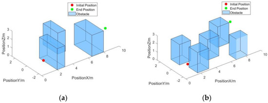
Figure 3.
The test environment. (a) Scenario 1. (b) Scenario 2.

Table 1.
Obstacle information for scenario 1.
Table 2.
Obstacle information for scenario 2.
4.1.2. Trajectory Generation Comparison
We use Fast-Planner and our method to generate trajectories based on the paths obtained by the A* algorithm, while recording the operation time, trajectory running time, trajectory length, and trajectory smoothness. The smoothness of the trajectory is evaluated by the integral of the square of the acceleration. Since the initial path is the same, the trajectories obtained by the two methods are determined. As shown in Figure 4, the blue dotted line is the initial path found by A*, the solid red line is the trajectory optimized by Fast-Planner, and the green dash–dotted line is the trajectory obtained by the proposed method. The results in Figure 5 and Figure 6 show that both trajectory optimization methods can obtain safe and smooth trajectories, but compared with the trajectory obtained by Fast-Planner, the trajectory obtained by the proposed method is shorter and smoother, which is more suitable for multi-rotor UAV execution.
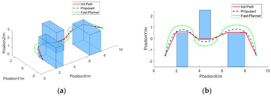
Figure 4.
Generated trajectory comparison in scenario 1. (a) Generated trajectories comparison. (b) Projection of the trajectories on the X–Y plane.
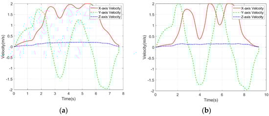
Figure 5.
Trajectory velocity curve comparison. (a) Proposed Method. (b) Fast-Planner.
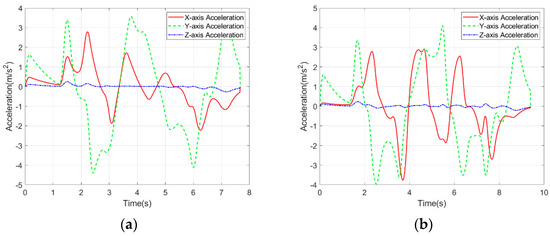
Figure 6.
Trajectory acceleration curve comparison. (a) Proposed Method. (b) Fast-Planner.
In order to conduct a quantitative analysis of the trajectory, this paper uses four variables, namely planning time, trajectory running time, length, and smoothness, as evaluation indicators. The smoothness of the trajectory is the mean value of the absolute value of the acceleration. The results are shown in Table 3. It can be seen from the results in the table that, compared with Fast-Planner, the proposed method adds safety distance calculation and dynamic adjustment steps. Hence, the planning time is slightly longer than Fast-Planner, but both can meet the real-time requirements of multi-rotor UAV motion planning. Compared with the trajectory obtained by Fast-Planner, the motion time of the trajectory obtained by the proposed method is reduced by 16.2% compared with Fast-Planner, the trajectory length is reduced by 16.25%, and the average acceleration is reduced by 7.98%. Therefore, the trajectory planned by the proposed method can make the UAV reach the target point more quickly and move more smoothly.
Table 3.
Experimental results of scenario 1.
In scenario 2, the trajectory generation method is shown in Figure 7. The blue dotted line is the initial path found by A*, the solid red line is the trajectory optimized by Fast-Planner, and the green dash–dotted line is the trajectory obtained by the proposed method. In scenario 2, Fast-Planner and the proposed method get a safe and smooth trajectory.
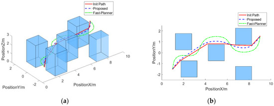
Figure 7.
Generated trajectory comparison in scenario 2. (a) Generated trajectories comparison. (b) Projection of the trajectories on the X–Y plane.
Figure 8 and Figure 9 show the planned trajectory velocity and acceleration curves of Fast-Planner and the proposed method in scenario 2. The experiment results show that the velocity and acceleration of the trajectory meet the dynamic requirements, the starting point and end point of the speed and acceleration meet the preset values, and the velocity and acceleration do not exceed the maximum limits of and . Therefore, both trajectories are dynamically feasible.
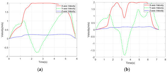
Figure 8.
Trajectory velocity curve comparison. (a) Proposed Method. (b) Fast-Planner.
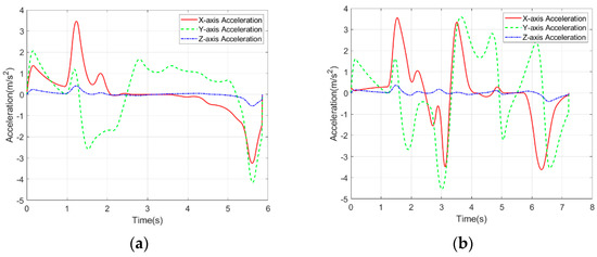
Figure 9.
Trajectory acceleration curve comparison. (a) Proposed Method. (b) Fast-Planner.
Scenario 2 also uses planning time, trajectory running time, trajectory length, and trajectory smoothness as evaluation indicators. The results are shown in Table 4. In scenario 2, compared with Fast-Planner, the proposed method still has obvious advantages in various indicators. The planning time of the two algorithms is approximately the same, which can meet the real-time requirements. However, the trajectory length and smoothness of the proposed method, are significantly less than Fast-Planner, so it is more suitable for multi-rotor UAV execution.
Table 4.
Experimental results of scenario 2.
4.2. Real-World Tasks
This section verifies the effectiveness of the proposed method in real-world tasks.
4.2.1. Flight Platform and Software Environment
This section implements the quadrotor shown in Figure 10 as the flight platform, which uses PX4 as the quadrotor control system and carries Dji Manifold 2 as the onboard computer. The processor model of Dji Manifold 2 is Intel I7-8850U, and the RAM size is 8 GB. The Intel RealSense tracking camera T265 provides reliable pose estimation for quadrotor, and the Intel RealSense depth camera D455 provides the depth image of the environment.
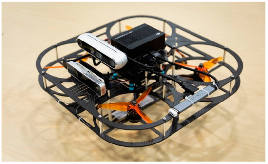
Figure 10.
Flight platform used in this section.
The operating system of the airborne computer is Ubuntu 18.04. UAV’s perception, path planning, and trajectory generation algorithms are developed using C++11 based on ROS (Robot Operating System). ROS is a widely used open-source robot system. It provides robot data communication interfaces, visualization tools, etc. Additionally, cameras and other hardware have also developed corresponding SDKs for ROS. The system software architecture diagram is shown in Figure 11. The system takes the posture and depth image provided by the binocular camera as input and builds the occupied grid map of the environment in real-time. When the target message is obtained, the path-planning algorithm searches for a feasible path in the map. Then, the trajectory generation algorithm generates a smooth continuous trajectory according to the path. Finally, the multi-rotor UAV control algorithm converts the trajectory to the control quantity, realizes the control of the quadrotor UAV based on MAVROS, and finally controls the multi-rotor UAV to reach the target position along the planned trajectory.
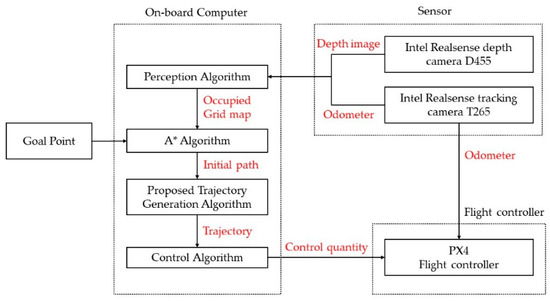
Figure 11.
The system software architecture diagram.
4.2.2. Experimental Environment and Related Settings
The test scene is indoors. The scene settings are shown in the Figure 12. The obstacle setting is shown in Table 5 and Table 6. In the test, the UAV realized positioning and environment perception based on onboard sensors and flew around obstacles to the target point. In order to thoroughly verify the effectiveness of the algorithm, this paper sets two groups of tests with different dynamic constraints. The maximum flight speed of both groups of tests is set to , and the maximum acceleration is set to .
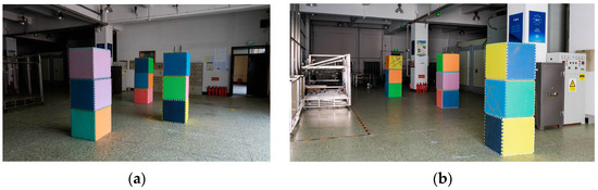
Figure 12.
Real-world task environment. (a) Sense 1. (b) Sense 2.
Table 5.
Obstacle information of sense 1.
Table 6.
Obstacle information of sense 2.
The mapping algorithm parameters are set as follows: the camera resolution is 848 × 480, the maximum measurement distance of the camera is 5.0 m, the minimum measurement distance is 0.3 m, and the obstacle determination threshold is 0.368. The parameters of the trajectory generation algorithm are set as follows: the optimization coefficients of the smooth item, the safety item, and the trajectory length item are set to 0.2, 0.15, and 0.025, respectively; the initial safety distance is set to 0.6 m; and the trajectory length penalty threshold is set to 0.2 m.
This paper’s perception, path planning, and trajectory generation algorithm can run in real time. Therefore, the experiment does not choose to conduct perceptual mapping and offline path planning in advance, but instead to sense in real-time and replan the trajectory by detecting collisions. In the initial stage, the unperceived area is the obstacle-free area by default. The system plans a safe path based on the algorithm and then uses the trajectory optimization algorithm proposed in this paper to optimize the path to obtain a safe and smooth ideal trajectory. During the flight process, the multi-rotor UAV perceives the obstacles to update the occupied grid map and detect the collision between the trajectory and the obstacles in real time. If the trajectory collides with the obstacles, it must replan it. The replanned trajectory takes the current UAV state as the starting state and the terminal point state as the target state. Based on the algorithm, the feasible path is re-searched, and then the algorithm proposed in this paper is used to obtain a safe and smooth trajectory to avoid obstacles. During the flight of the UAV, the trajectory safety is checked at the frequency of 10 Hz, and when the trajectory collides with the obstacle, it is replanned until the UAV reaches the target point.
4.2.3. Real-World Task Result
The experimental data of flight trajectories in senses 1 and 2 are shown in Figure 13, where the solid blue line is the trajectory of the UAV. Figure 14 is a series of screenshots of the actual flight video of the UAV. It can be seen that the UAV can avoid obstacles and smoothly fly to the preset destination. The maximum flight speed of the UAV in sense 1 is , and the maximum acceleration is , and the maximum speed of the UAV in sense 2 is , and the maximum acceleration is . The experimental results show that the trajectory generation algorithm proposed in this paper generates a safe and smooth trajectory that meets the dynamic requirements.
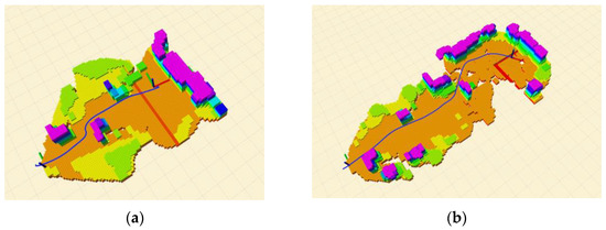
Figure 13.
Real-world task result. (a) Sense 1. (b) Sense 2.
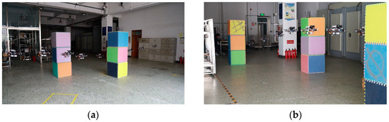
Figure 14.
Screenshot of flight video. (a) Sense 1. (b) Sense 2.
5. Conclusions
In this paper, an improved trajectory generation method is proposed, which calculates the security threshold based on the upper bound of the error between the B-spline curve and the control polygon, and then proposes a trajectory generation method with dynamic parameter adjustment. Compared with Fast-Planner, the method proposed in this paper significantly improves the trajectory quality. The simulation and real-world task results show that the proposed trajectory generation method can obtain a better trajectory.
Author Contributions
Conceptualization, K.W. and Z.M.; methodology, K.W.; software, K.W. and Z.W. (Zichen Wang); validation, K.W., Z.M. and Z.W. (Zhenping Wu); formal analysis, K.W.; investigation, Z.M.; resources, Z.M.; data curation, Z.W. (Zhenping Wu); writing—original draft preparation, K.W.; writing—review and editing, K.W. and Z.M.; visualization, Z.W. (Zichen Wang); supervision, Z.M.; project administration, Z.M.; funding acquisition, Z.M. All authors have read and agreed to the published version of the manuscript.
Funding
This research was funded by National Natural Science Foundation (NSF) of China (No. 61976014) and the Fundamental Research Funds for the Central Universities.
Institutional Review Board Statement
Not applicable.
Informed Consent Statement
Not applicable.
Data Availability Statement
The data presented in this paper are available on request from the first author.
Conflicts of Interest
The authors declare no conflict of interest.
References
- Dijkstra, E.W. A note on two problems in connexion with graphs. Numer. Math. 1959, 1, 269–271. [Google Scholar] [CrossRef]
- Hart, P.E.; Nilsson, N.J.; Raphael, B. A formal basis for the heuristic determination of minimum cost paths. IEEE Trans. Syst. Sci. Cybern. 1968, 4, 100–107. [Google Scholar] [CrossRef]
- Kavraki, L.E.; Svestka, P.; Latombe, J.C.; Overmars, M.H. Probabilistic roadmaps for path planning in high-dimensional configuration spaces. IEEE Trans. Robot. Autom. 1996, 12, 566–580. [Google Scholar] [CrossRef]
- Karaman, S.; Frazzoli, E. Sampling-based algorithms for optimal motion planning. Int. J. Robot. Res. 2011, 30, 846–894. [Google Scholar] [CrossRef]
- Mellinger, D.; Kumar, V. Minimum snap trajectory generation and control for quadrotors. In Proceedings of the 2011 IEEE International Conference on Robotics and Automation, Shanghai, China, 9–13 May 2011; pp. 2520–2525. [Google Scholar]
- Richter, C.; Bry, A.; Roy, N. Polynomial trajectory planning for aggressive quadrotor flight in dense indoor environments. In Robotics Research; Springer: Cham, Switzerland, 2016; pp. 649–666. [Google Scholar]
- Gao, F.; Wu, W.; Lin, Y.; Shen, S. Online Safe Trajectory Generation for Quadrotors Using Fast Marching Method and Bernstein Basis Polynomial. In Proceedings of the 2018 IEEE International Conference on Robotics and Automation (ICRA), Brisbane, QLD, Australia, 21–25 May 2018; pp. 344–351. [Google Scholar]
- Deits, R.; Tedrake, R. Efficient mixed-integer planning for UAVs in cluttered environments. In Proceedings of the 2015 IEEE International Conference on Robotics and Automation (ICRA), Seattle, WA, USA, 26–30 May 2015; pp. 42–49. [Google Scholar]
- Liu, S.; Watterson, M.; Mohta, K.; Sun, K.; Bhattacharya, S.; Taylor, C.J.; Kumar, V. Planning dynamically feasible trajectories for quadrotors using safe flight corridors in 3-d complex environments. IEEE Robot. Autom. Lett. 2017, 2, 1688–1695. [Google Scholar] [CrossRef]
- Campos-Macías, L.; Gómez-Gutiérrez, D.; Aldana-López, R.; de la Guardia, R.; Parra-Vilchis, J.I. A hybrid method for online trajectory planning of mobile robots in cluttered environments. IEEE Robot. Autom. Lett. 2017, 2, 935–942. [Google Scholar] [CrossRef]
- Chen, J.; Su, K.; Shen, S. Real-time safe trajectory generation for quadrotor flight in cluttered environments. In Proceedings of the 2015 IEEE International Conference on Robotics and Biomimetics (ROBIO), Zhuhai, China, 6–9 December 2015; pp. 1678–1685. [Google Scholar]
- Ren, Y.; Zhu, F.; Liu, W.; Wang, Z.; Lin, Y.; Gao, F.; Zhang, F. Bubble planner: Planning high-speed smooth quadrotor trajectories using receding corridors. In Proceedings of the 2022 IEEE/RSJ International Conference on Intelligent Robots and Systems (IROS), Kyoto, Japan, 23–27 October 2022; pp. 6332–6339. [Google Scholar]
- Zucker, M.; Ratliff, N.; Dragan, A.D.; Pivtoraiko, M.; Klingensmith, M.; Dellin, C.M.; Bagnell, J.A.; Srinivasa, S.S. CHOMP: Covariant hamiltonian optimization for motion planning. Int. J. Robot. Res. 2013, 32, 1164–1193. [Google Scholar] [CrossRef]
- Kalakrishnan, M.; Chitta, S.; Theodorou, E.; Pastor, P.; Schaal, S. STOMP: Stochastic trajectory optimization for motion planning. In Proceedings of the 2011 IEEE International Conference on Robotics and Automation, Shanghai, China, 9–13 May 2011; pp. 4569–4574. [Google Scholar]
- Oleynikova, H.; Burri, M.; Taylor, Z.; Nieto, J.; Siegwart, R.; Galceran, E. Continuous-time trajectory optimization for online UAV replanning. In Proceedings of the 2016 IEEE/RSJ International Conference on Intelligent Robots and Systems (IROS), Daejeon, Republic of Korea, 9–14 October 2016; pp. 5332–5339. [Google Scholar]
- Usenko, V.; Von Stumberg, L.; Pangercic, A.; Cremers, D. Real-time trajectory replanning for MAVs using uniform B-splines and a 3D circular buffer. In Proceedings of the 2017 IEEE/RSJ International Conference on Intelligent Robots and Systems (IROS), Vancouver, BC, Canada, 24–28 September 2017; pp. 215–222. [Google Scholar]
- Zhou, B.; Gao, F.; Wang, L.; Liu, C.; Shen, S. Robust and efficient quadrotor trajectory generation for fast autonomous flight. IEEE Robot. Autom. Lett. 2019, 4, 3529–3536. [Google Scholar] [CrossRef]
- Zhou, B.; Pan, J.; Gao, F.; Shen, S. Raptor: Robust and perception-aware trajectory replanning for quadrotor fast flight. IEEE Trans. Robot. 2021, 37, 1992–2009. [Google Scholar] [CrossRef]
- Zhou, X.; Wang, Z.; Ye, H.; Xu, C.; Gao, F. Ego-planner: An esdf-free gradient-based local planner for quadrotors. IEEE Robot. Autom. Lett. 2020, 6, 478–485. [Google Scholar] [CrossRef]
- Wang, Z.; Zhou, X.; Xu, C.; Gao, F. Geometrically constrained trajectory optimization for multicopters. IEEE Trans. Robot. 2022, 38, 3259–3278. [Google Scholar] [CrossRef]
- Nairn, D.; Peters, J.; Lutterkort, D. Sharp, quantitative bounds on the distance between a polynomial piece and its Bézier control polygon. Comput. Aided Geom. Des. 1999, 16, 613–631. [Google Scholar] [CrossRef]
- Reif, U. Best bounds on the approximation of polynomials and splines by their control structure. Comput. Aided Geom. Des. 2000, 17, 579. [Google Scholar] [CrossRef]
Disclaimer/Publisher’s Note: The statements, opinions and data contained in all publications are solely those of the individual author(s) and contributor(s) and not of MDPI and/or the editor(s). MDPI and/or the editor(s) disclaim responsibility for any injury to people or property resulting from any ideas, methods, instructions or products referred to in the content. |
© 2023 by the authors. Licensee MDPI, Basel, Switzerland. This article is an open access article distributed under the terms and conditions of the Creative Commons Attribution (CC BY) license (https://creativecommons.org/licenses/by/4.0/).