Featured Application
With the continuous development of the software industry, software is gradually becoming more inclined towards containerized deployment. This paper provides a prediction algorithm based on deep learning to monitor and record the resource usage of the machine and predict future resource usage so that the server can sense the future traffic load in advance and realize automatic scaling.
Abstract
In this paper, a deep learning-based prediction model VMD-GLRT is proposed to address the accuracy problem of service load prediction. The VMD-GLRT model combines Variational Mode Decomposition (VMD) and GRU-LSTM. At the same time, the model incorporates residual networks and self-attentive mechanisms to improve accuracy of the model. The VMD part decomposes the original time series into several intrinsic mode functions (IMFs) and a residual part. The other part uses a GRU-LSTM structure with ResNets and Self-Attention to learn the features of the IMF and the residual part. The model-building process focuses on three main aspects: Firstly, a mathematical model is constructed based on the data characteristics of the service workload. At the same time, VMD is used to decompose the input time series into multiple components to improve the efficiency of the model in extracting features from the data. Secondly, a long and short-term memory (LSTM) network unit is incorporated into the residual network, allowing the network to correct the predictions more accurately and improve the performance of the model. Finally, a self-focus mechanism is incorporated into the model, allowing the model to better capture features over long distances. This improves the dependence of the output vector on these features. To validate the performance of the model, experiences were conducted using open-source datasets. The experimental results were compared with other deep learning and statistical models, and it was found that the model proposed in this paper achieved improvements in mean absolute percentage error (MAPE).
1. Introduction
1.1. Background
In recent years, microservices have seen rapid development, and service containerization has become an increasingly popular method for deploying application services in the industry. Furthermore, an increasing number of software applications are being deployed to the cloud [1]. However, the load of a service is closely related to its function, meaning that services with different functions in different scenarios have different levels of load, and thus require additional hardware resources. However, hardware resources are often limited. To make the most of these resources, horizontal scaling should be employed when the service load is too high to reach the hardware resource utilization threshold.
Traditional monolithic applications cannot cope with the shortage of local resources and scalability dilemma. Therefore, the hybrid cloud has become a hot direction for current applications, but workflow scheduling is still a fundamental problem to be studied [2]. At the same time, the waste of resources caused by low service load cannot be ignored. These problems lead to the resources not being fully utilized, so there is a contradiction between the demand for software and hardware resources and the imbalance of utilization. Currently, the most popular cloud deployment management method is Kubernetes (K8s) cluster management, which allows for more precise resource configuration under the original processing method. As such, this paper is based on K8s as the foundation for service deployment. Finding the optimal load level for different services and resolving inefficient resource scheduling based on existing resource conditions to ensure efficient software operation is a complex problem.
To address these issues and ensure that the software maintains an appropriate resource allocation method across different periods, resource allocation is typically carried out in advance in the same historical period, relying on experience-based judgment. However, as software continues to evolve and update, a manual review can become a cumbersome task when there are too many services, compromising the accuracy of the decision, particularly when expanding traditional applications, resulting in a higher cost. Therefore, the value of using an empirical judgment approach is invaluable and far outweighs the benefits, which do not meet the current needs of microservice software development and deployment. Furthermore, incorrect predictions can lead to Service Level Agreement (SLA) violations, resulting in a significant waste of resources or system instability [3]. Accurately predicting the performance of application services is essential for effective scheduling and resource allocation, and can be beneficial for service migration and efficient resource allocation [4].
Exploring how to effectively leverage the fast response of edge servers and the powerful processing of global schedulers to address workflow scheduling problems has great potential for research [5]. Consequently, a prediction-based resource allocation is urgently needed to maximize the value of applications with limited resources [6].
1.2. Related Work
Service load data can typically be viewed as a time series analysis problem, which is typically approached from three perspectives: statistical methods, machine learning methods, and deep learning methods. To reduce the high maintenance costs associated with over-provisioning or under-allocating resources in the cloud environment, many recent studies have proposed solutions based on machine learning and deep learning to predict cloud host resource utilization.
1.2.1. Machine Learning
Machine learning has become increasingly popular among scholars due to its many advantages, such as the ability to train on large datasets and use labeling, prediction, and other operations to obtain a more accurate prediction model.
The study in [7] proposed an Evolutionary neural Network NN (ENN) that used Particle Swarm Optimization (PSO), Differential Evolution (DE), and the covariance matrix adaptive optimization evolution strategy. This method can predict more accurately in a short time, but in the long run, there is a decrease in accuracy. The study in [8] proposed an Automatic Regression Integrated Moving Average workload forecasting (ARIMA-PERP) model, which determined the best-fitting ARIMA model by minimizing Information Criterion, Enhanced Minimizing Information Criterion, and Bayesian Information Criterion (BIC). It realized the accurate advance of node load in advance, and the accuracy reached 91.11%. The study in [9] proposed a prediction method based on ensemble learning, which used the fast-learning ability of an Extreme Learning Machine (ELM) to reduce the consumption of training time, selected its weight based on a heuristic algorithm to predict the load of the cloud resources and improved the prediction accuracy compared with the traditional model. The study in [10] proposed a novel hybrid wavelet time series decomposition and GMMH-ELM ensemble method (WGE) for NFV workload prediction, which predicted and integrated workloads on different time-frequency scales. Compared with the traditional SVR and LSTM on multiple data sets, the MAPE was improved by about 8%. The study in [11] proposed a prediction method based on support vector regression, which used the historical host utilization of multiple resources to train support vector machines and realize prediction. Compared with the traditional linear regression prediction, Euclidean distance, and regression based on absolute sum, the proposed method performed better in many aspects, such as mean square error and fundamental percentage error. The study in [12] analyzed and compared the prediction results of more mainstream machine learning methods, such as linear regression and ElasticNet, with the Gated Recurrent Unit (GRU). The results show that it can provide superior prediction accuracy with increased data volume, which is contrary to the traditional machine learning methods. Therefore, it was concluded that the deep learning method is excellent for the conventional machine learning regression algorithm in time series modeling and can provide superior prediction accuracy.
1.2.2. Deep Learning
Deep learning methods have seen rapid growth in time series modeling, with many researchers taking advantage of their powerful capabilities and ability to automatically extract features to cope with time series.
The study in [13] proposed a load prediction method based on LSTM to improve network speed. This method considered the problem of insufficient resources in Edge Data Centers (EDC) and combined it with user mobility and geographical location information to improve prediction accuracy. Compared with the traditional statistical method, the accuracy of the proposed method increased by 4.21% on average. The study in [14] proposed a cloud workload prediction algorithm, L-PAW, based on deep learning. The model integrated the designed TSA and gated recurrent unit into RNN to achieve adaptive and accurate prediction of highly variable workloads. L-PAW achieves superior performance. The study in [15] proposed an integrated prediction method combining Bidirectional and Grid Long Short-Term Memory networks (BG-LSTM) to predict workload conditions and resource usage records. The Savitzky–Golay filter smoothed the model to eliminate noise. Experiments show that the model has good performance and adaptability. The study in [16] proposed a prediction model, CPW-EAMC, based on a noise reduction algorithm and neural network, which improved the robustness of the prediction algorithm through noise reduction, used a multidimensional prediction network, and comprehensively evaluated the model combined with the CMES evaluation standard. Compared with other popular methods, the performance was improved by up to 17%. The study in [17] established a deep learning module, SG-CBA, based on the Convolutional Neural Network (CNN) and Long Short-Term Memory network (BiLSTM) and integrated the filter and attention mechanism. Experiments were carried out on the accurate public data set of Alibaba. The results showed that compared with the traditional and more popular models, it could achieve better performance. Inspired by the translation of the long text, the study in [18] proposed a technology based on Attention-seq2seq to predict a load of cloud resources, which solved the problem of RNN forgetting critical information in long-term sequences and tested it on public data sets. Compared with other models, the accuracy was improved while the training time on the model was reduced, which showed the effectiveness of the current model. The study in [19] used the combination of GRU and LSTM to model the time series of node load data, selected the combination data of CPU and memory usage through the random forest, and used the combination model to predict it. The results showed that compared with traditional statistical methods, single deep learning methods, and combined prediction methods, the proposed method achieved good performance in prediction results. The study in [20] proposed a combined load forecasting method based on IF-EMD-LSTM (IEBL), which integrated the Isolation Forest algorithm (IF) and Empirical Mode Decomposition (EMD) into LSTM to improve the accuracy of forecasting. The experimental results showed that the error of the combined forecasting model was reduced by up to 18.72%. The prediction accuracy was higher than its corresponding single prediction model.
Many problems can be solved for time-series prediction: for example in the literature [21,22,23], where several prediction methods were proposed for a load of services. Additionally, under other application areas, for example in the literature [24,25,26], prediction methods have been proposed for PM (2.5), freight volumes, and so on. From the above analysis, it can be concluded that the combined prediction model always outperforms the single prediction model in terms of performance, both in terms of machine learning and deep learning. Moreover, many of the prediction models currently proposed for cloud computing load problems have improved performance compared to traditional prediction models, but their overall accuracy needs to be improved. Therefore, there is still an urgent need for a load prediction model with a high degree of accuracy to cope with such problems.
1.2.3. Contribution
This paper proposes a service load prediction method (VMD-GLRT) based on VMD and GRU-LSTM, based on the background of the above problem. This paper begins by modeling the problem based on service load prediction characteristics. The network structure was constructed based on the problem model to extract data features. Firstly, the input load data were decomposed into multiple signal feature components and the modal signals were modeled in time series. Secondly, the prediction results were corrected based on the residual blocks incorporated into the long and short-term memory network and a self-attentiveness mechanism was introduced, which can extract the features of the signal vector associated with the other, improving the generalization ability of the model. Finally, the final prediction results are derived by signal fusion. To verify the performance of the models, more recent and novel models in the field of time series processing were chosen for testing in this paper, and then the models are ablated and compared based on the same configuration with the same data set.
2. Materials and Methods
2.1. Model Building
In this paper, the result is assumed to be the output of a model component, with the load data decomposed into n components with a total of t features. The problem model is then formulated as (1) through formal description:
Service load is affected by many factors, with representing the actual load data and representing the component data, a part of the original data, after mode splitting. The component data are the result of the VMD decomposition, which represents a component of the original data, and we will refer to the VMD decomposition several times later when we discuss the VMD mode decomposition. The difference between the two is the residual sequence of the actual data. Since the components after modal decomposition cannot be entirely consistent with those before deterioration after merging, the difference between the accurate data and the sum of each component is regarded as the residual sequence of the load data and sent to the model for prediction. The prediction results of each other element are represented by , and the service load value at the next time point can be obtained by summing up the prediction results of all components, including the residual sequence.
The model utilizes the fast convergence ability of GRU and the prediction accuracy of LSTM to accurately extract the service’s load characteristics by decomposing the input signal into multiple variables using VMD. The overall structure of the model is shown in the following figure:
The model takes as input, where n is the number of feature vectors. Variational mode decomposition, feature extraction, and feature fusion are then applied to the input, resulting in the output of the corresponding prediction result sequence . Before the data can be input into the GRU, they need to be modally decomposed, as shown in the dashed box in Figure 1. The steps of the model processing are as follows:
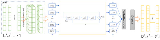
Figure 1.
Overall structure diagram of the model.
Firstly, the input data are preprocessed to form the initial input matrix , and the corresponding multivariate matrix of the data is obtained by modal decomposition for the single variable of the input data. The formal expression is shown as Equation (2), where n is the number of components and m is the dimension of the feature vector.
Secondly, the variables after the modal decomposition of each variable are recombined according to the order of the components of the modal decomposition to form the input features. Then, the GRU is used for feature extraction, and then the residual block based on LSTM is corrected and sent to LSTM to obtain accurate prediction results.
Finally, the correlation distance between each component is shortened through the self-attention mechanism, and the correlation relationship between each element is fully extracted. The final prediction sequence can be obtained through feature fusion. The relevant details are presented in the following, where 2.2 is the modal decomposition process and 2.3 is the prediction process.
2.2. Signal Decomposition Method and Process
Before the data are input into the GRU, considering that different services show different business characteristics under the load, and the model feature extraction will also affect the model’s performance, the model’s data characteristics should show certain regularity, highlighting its business-aware characteristics. Therefore, in this paper, the input data are decomposed by variational mode decomposition. In this paper, it is assumed that any set of load sequences is composed of multiple variables , and is the center band frequency of each component, where k is the component sequence number of mode decomposition. For each set of input service load data,
- Firstly, is transformed by Hilbert transform to obtain the analysis signal and its center band is modulated:
- The squared norm L2 of the modulation center band is calculated and the bandwidth of each IMF is estimated as follows:
- To find the optimal solution to the original problem, the Lagrange multiplier λ(t) and the factor α are introduced in the current step, and the problem is transformed into an unconstrained variational problem with the Lagrange operator and quadratic penalty term, which is formalized as follows:
- Finally, the alternating direction method of multipliers is used to continuously update each component and its center frequency, and the solution to the original problem can be obtained. It is updated as follows:
On the symbol of , respectively, corresponding , s(t) and and the Fourier transform of lambda (t).
- Based on the above analysis results, the algorithm re-estimates the center frequency:
- Initialize and n;
- execute cycle n = n + 1;
- When , update according to (6);
- update and . The formula is given below:
- When the accuracy (calculated as shown in Equation (9)) reaches a given constraint value ε and the component has reached k components, the algorithm is exited, and the optimal modal component is thus obtained. The symbol ε above is the precision of the iteration, and when ε is less than 1 × 10⁻⁶, this results in the push-out condition.
After the algorithm is executed, the components of the mode decomposition can be obtained from the optimization results. To account for errors in the modal variables and different conditions of service loads, the original sequence is obtained by accumulating the components obtained after modal decomposition with the original data, and it is directly sent to the model for prediction to obtain more accurate prediction results. This is the processing process before feeding into the model, as shown in the front part of GRU in Figure 1.
2.3. The Residual Structure of Long-Term Memory
To accurately predict the future form of features under other business-aware characteristics in microservices, where the behavior of the service load is different, this paper introduces a gated neural network to extract the features of the input data, allowing the model to converge quickly. To avoid the problem of model degradation and long-term memory loss caused by depth, LSTM and the convolutional layer are combined to form the residual block. The self-attention mechanism is integrated to further improve the accuracy of prediction by enhancing the depth of the model and the correlation between the model and historical data, thus obtaining the characteristics of the load data accurately. As shown in the right-hand part of the dotted box in Figure 1.
For each input service load data , feature extraction is first performed through GRU, followed by residual correction through multi-layer residual blocks. The residual sequence is then learned and merged with the original sequence to obtain a more accurate result, which is then input into LSTM to receive the output result of the model. The residual connection structure diagram is shown in Figure 1 in the yellow box, while the model structure is shown in Figure 2. GRU is composed of an update gate and reset gate, and LSTM is composed of an input gate, output gate, and forget gate.
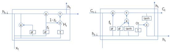
Figure 2.
Structure diagram of GRU (left) and LSTM (right) network units.
This paper combines multiple GRU units to achieve preliminary model feature extraction. For any set of service load data , it is directly input into the gating unit. Then, with the last unit output logic operation, it aims to ensure the memory of important information. Its forgetting process (Equation (10)) and memory process (Equation (11)) is expressed as follows.
where X is the service load data, H is the output of the gating unit at the last time, W is the weight value that should be questioned or remembered at the corresponding time, and b is the bias value. The memory and forgetting capabilities of the gated unit can be provided by calculation, and the results of the two will directly affect the feature extraction of the next unit. Therefore, the final processing result can be obtained by fusing the output with the hidden state. The calculation is as follows, as shown in (12):
⨀ symbol according to the elements multiplication.
To improve the accuracy of the model, the results of the above calculations are fed into the residual block of the LSTM. Let the output of the upper layer network be and be the desired output of the residual network, while this paper builds the following mathematical model based on the current assumptions, as shown in (13):
where f(x) is the residual sequence fit and x is the feature sequence of the LSTM. In the model, the characteristics of the key information should not be forgotten, so that the forgetting process can be constructed, as shown in (14).
Since the update gate is similar in structure to the forget gate, the only differences between the two are the weights and biases, so can be expressed as shown in (15). Similarly, the output gate is the same, differing only in weight and bias. While the forgotten gate is processed, the original signal is concatenated and scaled to obtain , as shown in (16).
According to Figure 2, is obtained by forgetting the non-critical information, multiplying the input data with the scaled data after the update operation, and adding it to the result of multiplying the previous state with the forgetting gate to obtain the current output . A formal expression is shown in (17).
Finally, the output gate is multiplied by the scaling of the output result, which is then fed into the convolution layer for convolution, and the result is fed into the LSTM network to produce the final prediction result of the model.
For a long time in input time series, RNN still has the problem of forgetting, and the model is challenging to extract the feature relationship between distant vectors, which leads to incomplete feature extraction of historical load data, and makes the trained model produce poor performance. From the sequence analysis, the input of this paper is multidimensional, and the result sequence is mainly a new sequence obtained by combining the CPU and memory usage at a specific time. Since CPU and memory usage is related to metrics such as network requests and disk IO operations, this paper considers the combined input of associated sequences.
Considering the above problems, this paper introduces the self-attention mechanism to extract the relationship features between different input vectors. For any input time series {Xn} containing multidimensional features, each input vector x corresponds to the output of a y, and each input variable x needs to be tested for the correlation of historical input vectors. In short, each input vector will be associated with the history vector through the self-attention mechanism when corresponding to the output vector, shorten the relationship with the long-distance vector, and extract as many features as possible to improve the accuracy of model training. Its structure diagram is shown in Figure 3 below.
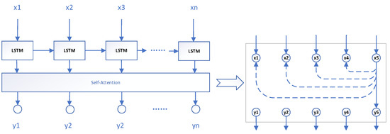
Figure 3.
Structure diagram of the self-attention mechanism.
3. Result and Discussion
3.1. Data Acquisition and Processing
To test the prediction performance of the model proposed in this paper, Alibaba’s open-source service load data Cluster-trace-v2018 is selected as the data set [21], which contains the machine load data of more than 4000 machines for eight days. In this paper, the resource usage of an apparatus for eight days is selected, and a total of 3300 load data are used as the data set. The combination of CPU and memory resource utilization is used to load data [27]. At the same time, the data of multiple dimensions, such as network usage and disk IO, are also included to form a data set. The cross-validation method is used for verification, and the last 300 records are used as the verification set to verify the model’s generalization ability.
First of all, because different software services have other performance characteristics in different application scenarios, even on various modules of the same software, there will be many differences in their load conditions. Therefore, in this paper, before using the data, firstly, for the unstable sequence, the VMD mode decomposition is used to divide the multidimensional features into multiple relatively stationary IMF components so that they tend to be relatively stationary. This paper’s decomposition effect of the prediction divided into five modes and feature combination columns is shown in Figure 4 below. The first layer is the original sequence, and the following five layers are the data after modal decomposition.
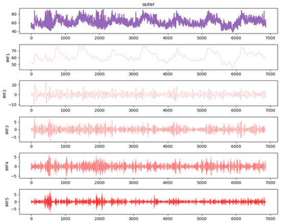
Figure 4.
Before and after mode decomposition.
Referring to the method in the study in [28], the IMF is set to 5 components. As shown in Figure 4, IMF1-IMF5 are data from different center frequency bands. Since it is not possible to completely decompose each time, there is always some error in the result. Assuming that IMFres is the residual sequence after the decomposition of the original sequence, the difference between the original sequence and the decomposed sequence is the value of the residual sequence IMFres. This paper considers that IMFres is also an additional component of the modal decomposition, except that the current component is not derived directly from the algorithm, but from the difference between the original sequence and the already decomposed variables.
3.2. Experiments and Results
Based on the above processing results, ablation and comparison experiments are conducted in this paper to test the influence of the GRU-LSTM model with residual block and attention mechanism on the prediction results. Comparative experiments are conducted to compare the model proposed in this paper with the statistical methods, deep learning methods, and other recent research models, and the prediction performance of the model is analyzed by comparing various evaluation indicators of the prediction results. Quantitative evaluation and comparison of the model evaluation indicators are conducted using MSE, RMSE, MAE, and MAPE.
The experimental process of this paper mainly includes four parts: data processing and parameter setting, prediction, result processing, and evaluation and comparison. To make the experimental results more accurate and comparable, all the model parameters are set uniformly in this paper, and the parameters are shown in Table 1. The experimental content is mainly divided into ablation experiments and contrast experiments. In this paper, the batch size is 32, the hidden layer in LSTM is 128, the learning rate is 0.00065, the number of iterations is 400, the step size of the sliding window is 1, and the IMF is the number of modal decompositions with five components.

Table 1.
Model configuration item Settings.
3.2.1. Ablation Experiment
Since this paper is optimized and upgraded based on the GRU-LSTM combined model, in this experiment, the integrated model of GRU-LSTM is used as the basic module as the basic model. At the same time, the residual block and the self-attention mechanism module are added and, finally, the signal decomposition is carried out. The prediction results are fused to obtain the final prediction results. Ablation experiments are performed based on the same data set and configuration. The comparison results are shown as follows (Figure 5):
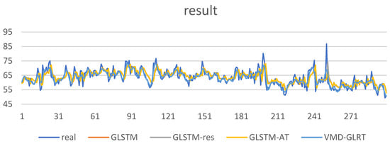
Figure 5.
Model prediction results for ablation experiments.
It can be seen from Figure 5 that the performance of the model in this paper is improved compared with the original model. From the trend point of view, the model’s accuracy is better than the original GRU-LSTM model after adding the module, and the error rate is reduced. To more accurately describe the new energy of the model, this paper records the experimental ablation model’s experimental evaluation index results and the evaluation index of different models, as shown in Table 2 below. The bold one is the algorithm of this paper, and the underlined one is the optimal result.
Table 2.
Evaluation indexes of ablation experiments.
At the same time, it can also be concluded from the table that the MSE of GRU-LSTM on the test set is 19.8621, and the MAPE is 5.06%. GLSTM-RS combines the residual structure based on LSTM to deepen the depth of the network, so its MSE on the validation set is 19.7945, which is slightly improved compared with the performance of the original model, which can show that the introduced residual block is helpful to improve the performance of the model. Based on introducing the residual structure, GLSTM-RT incorporates the self-attention mechanism. From the analysis of the experimental structure, it can be seen that the MSE of the model is 19.6048. Compared with the original model and the results integrated with the residual network, the error is reduced, and the accuracy is improved. It can be seen that the introduction of the self-attention mechanism can shorten the distance between the input vector and the historical vector in time series prediction to improve the accuracy of the model.
3.2.2. Comparative Experiment
Based on the previous analysis, this paper lists the existing combination models for experiments and comparison from three aspects of statistical methods, machine learning, and deep learning. To verify the effectiveness of the model, this paper will test and compare other prediction models in the field and prediction methods in service load prediction. The prediction result graph is shown in Figure 6 below.
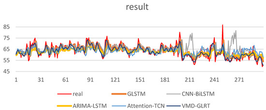
Figure 6.
Model prediction results for Comparative experiments.
Figure 6 shows that the prediction results of each model can be consistent with the primary trend under the premise of the same environment and setting. Comparing the proposed model with its base reference model, GRU-LSTM, the MAPE phase is improved by about 2%. To verify the model’s generalization ability, the model in this paper is predicted and compared with CNN-BiLSTM, ARIMA-LSTM, and Attention-TCN, which are novel models in recent studies from two aspects of statistical methods and deep learning methods. It can be seen from the results that the model proposed in this paper has a better prediction effect on the whole and is superior to other models in terms of trend and accuracy.
To further illustrate the prediction performance and effect of the model, this paper evaluates the model based on the four evaluation indicators of MSE, RMSE, MAE, and MAPE, and the results of each item are shown in Table 3 below. The bold one is the algorithm of this paper, and the underlined one is the optimal result.
Table 3.
Experimental comparison results.
Compared with the GRU-LSTM model proposed in the literature [27], the model presented in this paper has dramatically improved in all indicators. It can be seen from the data in the table that compared with the evaluation index results obtained by the recent model on the validation set, the prediction model proposed in this paper can achieve a more accurate performance. The study in [25] uses three proportions of equal weight average, differential reciprocal, and objective assignment to merge the prediction results of the combined model and obtain the optimal result. This paper compares the optimal results obtained under the differential typical weight setting method. The results show that the MAPE of this prediction method is increased by about 2.4% compared with this result. The MSE is reduced by about 13.5538, reducing the model’s error rate. Compared with the prediction results of the study in [26], the MAPE of this paper is reduced by about 3%, and the MSE is reduced by about 18.036, which dramatically improves its accuracy. On the same data set, compared with the method of visualizing time series and extracting and predicting features through CNN and LSTM proposed by the study in [23], this paper uses the same data set for prediction and comparison, and it can be seen that the proposed model in this paper reduces MAE by about 1.8837. It can be seen that the prediction results of the proposed model are closer to the actual value.
Through the above analysis, the model in this paper is superior to the existing statistical prediction methods and deep learning prediction methods in terms of evaluation indicators. In actual situations, the model can effectively deal with the differences in service load characteristics of different software in different scenarios and provide a reliable service load prediction scheme to help the industry predict the load demand of various services in different application scenarios in the future, provide response preparation for software practitioners, and make policy warnings in advance.
4. Conclusions
This paper proposes a service load prediction model, VMD-GLRT, based on VMD, to address the issue of inaccurate prediction results of current deep learning models. The model uses VMD to decompose the unstable time series data into modal components that tend to be stable, thus facilitating the extraction of features. Additionally, the self-attention mechanism and residual network are introduced to improve the accuracy of the prediction results. Ablation experiments and comparison experiments were conducted to verify the effectiveness of the model, and the results show that the proposed model has better generalization ability, improves the accuracy of load prediction, and meets the demand of industry for service load prediction, allowing for reasonable resource allocation of services in advance.
Author Contributions
Conceptualization, J.Z.; Methodology, J.Z.; Validation, Y.P., C.S., W.C. and Y.H. (Yuanyuan Huang); Writing—original draft, Y.H. (Yiqi Huang); Writing—review & editing, Y.H. (Yiqi Huang). All authors have read and agreed to the published version of the manuscript.
Funding
This research was funded by the Scientific and Technological Progress and Innovation Program of the Transportation Department of Hunan Province (201927), the Natural Science Foundation of Hunan Province (2021JJ30456, 2022JJ40514, 2022JJ90018, 2022JJ30624), the Open Fund of National Engineering Research Center of Highway Maintenance Technology (KFJ220107), the Open Research Project of the State Key Laboratory of Industrial Control Technology (No. ICT2022B60), National Defense Science and Technology Key Laboratory Fund Project (2021-KJWPDL-17).
Institutional Review Board Statement
Not applicable.
Informed Consent Statement
Not applicable.
Data Availability Statement
The dataset for this study is available on GitHub at https://github.com/alibaba/clusterdata (accessed on 1 July 2022).
Conflicts of Interest
The authors declare no conflict of interest.
References
- Larrucea, X.; Santamaria, I.; Colomo-Palacios, R.; Ebert, C. Microservices. IEEE Softw. 2018, 35, 96–100. [Google Scholar] [CrossRef]
- Liu, P.; Liu, B.; Zhou, N.; Peng, X.; Lin, W. Survey of Hybrid Coud Wlorkflow Sheduling. Comput. Sci. 2022, 49, 235–243. [Google Scholar]
- Amiri, M.; Mohammad-Khanli, L. Survey on prediction models of applications for resources provisioning in cloud. J. Netw. Comput. Appl. 2017, 82, 93–113. [Google Scholar] [CrossRef]
- Kazanavičius, J.; Mažeika, D. Migrating legacy software to microservices architecture. In Proceedings of the 2019 Open Conference of Electrical, Electronic and Information Sciences (eStream), Vilnius, Lithuania, 25 April 2019; IEEE: New York, NY, USA, 2019; pp. 1–5. [Google Scholar]
- Yu, H.; Liu, B.; Zhou, N.; Lin, W.; Liu, P. Survey of Multi-cloud Workflow Scheduling. Comput. Sci. 2022, 49, 250–258. [Google Scholar]
- Wang, Z.; Zhang, L.; Lv, B.; Ji, Y.; Hu, C.; Wen, S. Review of cloud computing resource scheduling based on machine learning. Radiocommun. Technol. 2022, 48, 213–222. [Google Scholar]
- Mason, K.; Duggan, M.; Barrett, E.; Duggan, J.; Howley, E. Predicting host CPU utilization in the cloud using evolutionary neural networks. Future Gener. Comput. Syst. 2018, 86, 162–173. [Google Scholar] [CrossRef]
- Gadhavi, L.J.; Bhavsar, M.D. Adaptive cloud resource management through workload prediction. Energy Syst. 2019, 13, 601–623. [Google Scholar] [CrossRef]
- Kumar, J.; Singh, A.K.; Buyya, R. Ensemble learning based predictive framework for virtual machine resource request prediction. Neurocomputing 2020, 397, 20–30. [Google Scholar] [CrossRef]
- Jeddi, S.; Sharifian, S. A hybrid wavelet decomposer and GMDH-ELM ensemble model for Network function virtualization workload forecasting in cloud computing. Appl. Soft Comput. 2020, 88, 105940. [Google Scholar] [CrossRef]
- Nehra, P.; Nagaraju, A. Host utilization prediction using hybrid kernel based support vector regression in cloud data centers. J. King Saud Univ.-Comput. Inf. Sci. 2021, 34, 6481–6490. [Google Scholar] [CrossRef]
- Khan, T.; Tian, W.; Ilager, S.; Buyya, R. Workload forecasting and energy state estimation in cloud data centres: ML-centric approach. Future Gener. Comput. Syst. 2022, 128, 320–332. [Google Scholar] [CrossRef]
- Guo, Q.; Huo, R.; Meng, H.; Xinhua, E.; Liu, J.; Huang, T.; Liu, Y. Research on LSTM-based load prediction for edge data centers. In Proceedings of the 2018 IEEE 4th International Conference on Computer and Communications (ICCC), Chengdu, China, 7–10 December 2018; IEEE: New York, NY, USA, 2018; pp. 1825–1829. [Google Scholar]
- Chen, Z.; Hu, J.; Min, G.; Zomaya, A.Y.; El-Ghazawi, T. Towards accurate prediction for high-dimensional and highly-variable cloud workloads with deep learning. IEEE Trans. Parallel Distrib. Syst. 2019, 31, 923–934. [Google Scholar] [CrossRef]
- Li, S.; Bi, J.; Yuan, H.; Zhou, M.; Zhang, J. Improved LSTM-based prediction method for highly variable workload and resources in clouds. In Proceedings of the 2020 IEEE International Conference on Systems, Man, and Cybernetics (SMC), Toronto, ON, Canada, 11–14 October 2020; IEEE: New York, NY, USA, 2020; pp. 1206–1211. [Google Scholar]
- Zhang, Y.; Liu, F.; Wang, B.; Lin, W.; Zhong, G.; Xu, M.; Li, K. A multi-output prediction model for physical machine resource usage in cloud data centers. Future Gener. Comput. Syst. 2022, 130, 292–306. [Google Scholar] [CrossRef]
- Chen, L.; Zhang, W.; Ye, H. Accurate workload prediction for edge data centers: Savitzky-Golay filter, CNN and BiLSTM with attention mechanism. Appl. Intell. 2022, 52, 13027–13042. [Google Scholar] [CrossRef]
- Al-Sayed, M.M. Workload Time Series Cumulative Prediction Mechanism for Cloud Resources Using Neural Machine Translation Technique. J. Grid Comput. 2022, 20, 16. [Google Scholar] [CrossRef]
- He, X.; Xu, J.; Wang, B.; Wu, H.; Zhang, B. Research on cloud computing resource load prediction based on GRU-LSTM combination model. Comput. Eng. 2022, 48, 11–17+34. [Google Scholar]
- Guo, L.; Qian, C. CPU load prediction of data center based on IF-EMD-LSTM. Comput. Simul. 2022, 39, 37–41+370. [Google Scholar]
- Guo, J.; Chang, Z.; Wang, S.; Ding, H.; Feng, Y.; Mao, L.; Bao, Y. Who limits the resource efficiency of my datacenter: An analysis of alibaba datacenter traces. In Proceedings of the International Symposium on Quality of Service, New York, NY, USA, 24–25 June 2019; pp. 1–10. [Google Scholar]
- Patel, E.; Kushwaha, D.S. A hybrid CNN-LSTM model for predicting server load in cloud computing. J. Supercomput. 2022, 78, 1–30. [Google Scholar] [CrossRef]
- Wang, Y.; Yu, L.; Teng, F.; Song, J.; Yuan, Y. Resource load prediction model based on long-short time series feature fusion. J. Comput. Appl. 2022, 42, 1508–1515. [Google Scholar]
- Rushan, Y.; Haibo, W. PM2.5 concentration prediction method based on CNN-BiLSTM model. Math. Pract. Theory 2022, 52, 181–188. [Google Scholar]
- Yan, Y.; Qing, H.; Si, L.; Pan, Z.; Ouyang, X. Research on Cargo Volume Combination Forecasting Method Based on ARIMA-LSTM. Traffic Sci. Eng. 2022, 38, 102–108. [Google Scholar]
- Wang, J.; Gao, Z.; Shan, C. Multivariate yellow river runoff prediction based on TCN-Attention model. Peoples Yellow River 2022, 44, 6. [Google Scholar]
- Zharikov, E.; Telenyk, S.; Bidyuk, P. Adaptive workload forecasting in cloud data centers. J. Grid Comput. 2020, 18, 149–168. [Google Scholar] [CrossRef]
- Liu, Y. Research on Short Term Power Load Forecasting Based on VMD and Improved LSTM; Hubei University of Technology: Wuhan, China, 2020. [Google Scholar]
Disclaimer/Publisher’s Note: The statements, opinions and data contained in all publications are solely those of the individual author(s) and contributor(s) and not of MDPI and/or the editor(s). MDPI and/or the editor(s) disclaim responsibility for any injury to people or property resulting from any ideas, methods, instructions or products referred to in the content. |
© 2023 by the authors. Licensee MDPI, Basel, Switzerland. This article is an open access article distributed under the terms and conditions of the Creative Commons Attribution (CC BY) license (https://creativecommons.org/licenses/by/4.0/).